


 Abstract
 HTML
HTML Reference
 Related
 PDF
PDF


-
The radioactive nucleus attains a stable configuration via the emission of mass or energy, and this process is known as radioactivity. The radioactive emission includes different decay modes, such as γ-decay, β-decay, α-decay, cluster radioactivity (CR), heavy particle radioactivity (HPR), and spontaneous fission (SF) [1−12]. These decay modes are generally found in nuclei belonging to the heavy and super-heavy mass regions [13, 14]. An interesting property of such nuclei is that they can decay via one or multiple channels of the above decay modes. Therefore, it is important to conduct a comparative analysis of these decay modes in terms of different nuclear properties, such as shape, size, magicity, the decay constant, and the decay half-lives [15, 16]. In the past few decades, different experimental and theoretical approaches [17−29] have been employed to explore such decay modes. Numerous theoretical models, such as the analytical superasymmetric model (ASAFM) [ 30, 31], unified fission model (UFM) [21–25], preformed cluster model (PCM) [26–29], density dependent cluster model (DDCM) [32, 33], two potential approach (TPA) [34–36], generalized liquid drop model (GLDM) [37–39], and many other approaches [40–42], have been introduced, which successfully explain the radioactive emission of a variety of fragments.
In the ASAFM, the decay constant and decay half-life are calculated using the barrier penetration probability and assault frequency. The preformation hypothesis is not exercised in the ASAFM. Using this model, [43] the decay half-lives have been found to strongly depend on the Q-value of the decay channel, and it was observed that a 5%-10% change in the Q-value altered the half-lives by a order of magnitude. Similarly, the significance of the Q-value was explored in Ref. [44], where the alpha decay was studied in reference to superheavy nuclei. The preformation and penetration effects were incorporated in Ref. [45] using the pre- and post-touching regions of the decaying fragments, and their Q-value dependent relations were obtained. One may note that the preformation and penetration probabilities depend on the Q-value of the decay channel and consequently affect the decay half-lives [46]. In contrast, the PCM explores different ground state decay mechanisms and is based on the collective mass clusterization approach, where the probable binary fragments are treated on equal footing [47, 48].
In view of this, γ and β- decay are not studied using this model. In general, stability analysis of radioactive nuclei are conducted in terms of the decay constant and decay half-life. The decay constant is obtained using the preformation probability
$ P_o $ , barrier penetrability P, and classical assault frequency$ v_o $ . The$ P_o $ value is calculated by solving the Schrödinger equation in terms of the mass asymmetry coordinate, and P is calculated in three steps using the Wentzel Kramers-Brillouin (WKB) approximation. Both the$ P_o $ and P values are computed at a turning point R=$ R_a $ , which is the sum of the radii of the decaying fragments at touching configurations and the neck length parameter ($ \Delta R $ ). As discussed earlier, the Q-value of the decay channel plays an important role in the calculation of$ P_o $ and P. Hence, in this study, the preformation probability and penetrability are calculated at the Q-value dependent$ R_a $ point, i.e.,$ R_a $ (Q). In a previous study by one of us and collaborators [6], the SF properties of 45 nuclei were investigated, where the most probable SF channels were identified and the importance of the neutron and proton shell closure effects were explored. In the current study, an attempt is made to comparatively analyze alpha decay and SF using a new set of binding energies [49]. Additionally, the α, CR, and HPR modes are analyzed by incorporating the Q-value effects into the first turning point$ R_a $ . The aim of this study is to (i) establish a Q-value dependent relation ($ R_a $ (Q)) for the α decay, CR, and HPR modes and explore the behavior of associated properties, (ii) study the Q-value, preformation probability, penetration probability, and decay half-lives of nuclei as functions of mass number using the$ R_a(Q) $ relation, (iii) conduct an SF mass distribution analysis using the spherical and hot configuration of the$ \beta_2 $ -deformed fragments, and (iv) study the total kinetic energy (TKE) of fission fragments. The paper is organized as follows. A description of the PCM is given in Sec. II, calculations and discussions are given in Sec. III, and the study is summarized in Sec. IV. -
The PCM is based on quantum mechanical fragmentation theory (QMFT) [50−53], where the cluster is supposed to be in a preformed state inside the parent nucleus. The model mainly operates in terms of the mass asymmetry coordinate and relative separation coordinate R. The probability of this preformation state of a cluster with respect to other probable clusters is called the preformation probability, which can be calculated by solving Schrödinger's wave equation in the η (mass asymmetry) co-ordinate and written as
$ \begin{equation} \left\{-\frac{\hbar^2}{2\sqrt{B_{\eta\eta}}}\frac{\partial}{\partial\eta} \frac{1}{\sqrt{B_{\eta\eta}}}\frac{\partial}{\partial\eta}+V_R(\eta,R) \right\}\psi^\nu(\eta)=E^\nu\psi^\nu(\eta), \end{equation} $

(1) where
$\nu=0,1,2,3,...$ refer to ground state$ (\nu=0) $ and excited state$ (\nu\neq0) $ solutions. For the case of the ground state, the preformation probability$ P_o $ is given as$ \begin{equation} P_o = |{\psi[\eta(A_i)]|^2}\sqrt{B_{\eta\eta}}\frac{2}{A_{\rm CN}}. \end{equation} $

(2) The mass parameters
$ {B_{\eta\eta}} $ (η) are the classical hydrodynamical masses of Kröger and Scheid [53] given for homogeneous radial mass flow. The potential in Eq. (1) is given as$ \begin{aligned}[b] V_R(\eta,R)=&\sum\limits_{i=1}^{2} B(A_i,Z_i)+V_C(R,Z_i,\beta_{\lambda i},\theta_i)\\ &+V_P(R,A_i,\beta_{\lambda i},\theta_i). \end{aligned} $

(3) Here,
$ B(A_i,Z_i $ ) are the binding energies of decaying fragments and are taken from Ref. [49], and when not available, are taken from [54]. The second and third terms in$ V_R $ represent the Coulomb and nuclear proximity potentials, respectively. For the case of deformed and oriented interacting nuclei, the expression for the Coulomb potential is$ \begin{aligned}[b] V_C(Z_i,\beta_{\lambda i},\theta_i,\alpha_i) = & \frac{Z_1Z_2{\rm e}^2}{R}+3Z_1Z_2{\rm e}^2\sum\limits_{\lambda,i=1,2}\frac{1}{2\lambda+1}\frac{R_i^{\lambda}(\alpha_i)}{R^{\lambda+1}} \\ &\times Y_{\lambda}^{(0)}\left[\beta_{\lambda i}+\dfrac{4}{7}\beta_{\lambda i}^2Y_{\lambda}^{(0)}(\theta_i)\right]. \end{aligned} $

(4) Moreover, the expression for two interacting spherical nuclei in Eq. (4) can be written as
$V_C(R)=\dfrac{Z_1Z_2{\rm e}^2}{R}$ . The nuclear proximity potential is given as$ \begin{equation} V_{Pij}(s)=4\pi \overline{R}\gamma b\Phi(s). \end{equation} $

(5) A detailed explanation of the proximity potential can be found in Ref. [55]. Furthermore, the barrier penetration probability probability P is calculated using the WKB integral and written as
$ \begin{equation} P=P_aW_iP_b. \end{equation} $

(6) The penetrability is calculated in three steps:
(i) The penetrability
$ P_a $ from$ R_a $ to$ R_i $ $ \begin{equation} P_a={\rm exp}[-\frac{2}{\hbar}\int_{R_a}^{R_i}\{2\mu[V(R)-V(R_i)]\}^{1/2}{\rm d}R], \end{equation} $

(7) (ii) the inner de-excitation probability
$ W_i $ at$ R_i $ (taken to be unity in reference to [56]),$ \begin{equation} W_i={\rm exp}(-bE_i), \end{equation} $

(8) (iii) the penetrability
$ P_b $ from$ R_i $ to$ R_b $ $ \begin{equation} P_b={\rm exp}[-\frac{2}{\hbar}\int_{R_i}^{R_b}\{2\mu[V(R)-Q]\}^{1/2}{\rm d}R]. \end{equation} $

(9) This three step penetration process is shown in Fig. 3. It may be noted that R=
$ R_a $ is the first (inner) turning point, and R=$ R_b $ is the second (outer) turning point calculated from the condition$ V(R_b $ )=Q-Value. This means that tunneling begins at R=$ {\rm{R}}_a $ and terminates at R=$ R_b $ .$ R_a $ (Q) and R$ _a $ ($ \Delta R $ ) are the points obtained using this relation (discussed in Sec. III). Here, the$ R_a $ point plays an important role in the decay analysis and is calculated as$ R_a $ =$ R_1 $ +$ R_2 $ +$ \Delta R $ (=$ R_t $ +$ \Delta R $ ), where$ R_t $ is the relative separation at the touching configuration. The fragment radii can be calculated via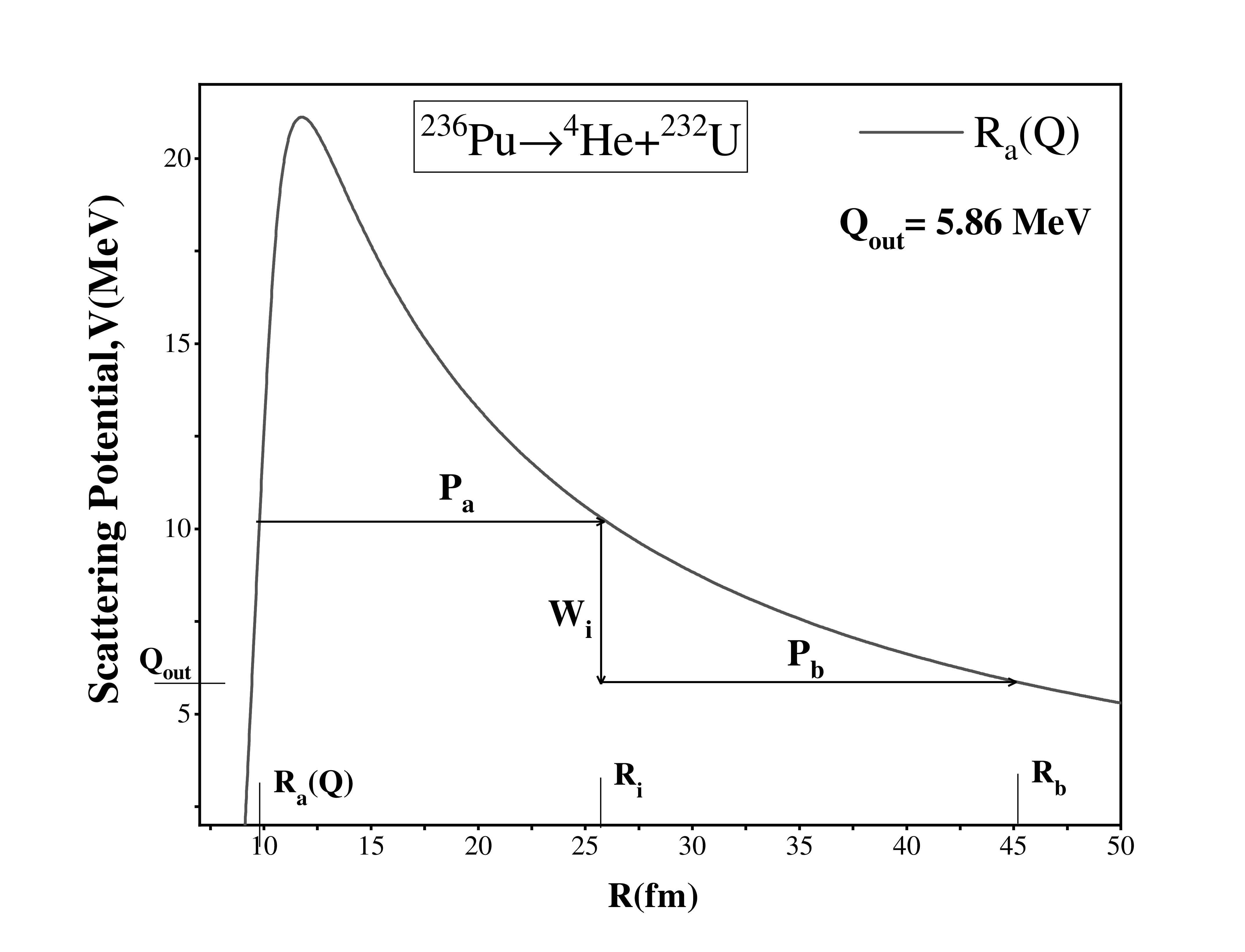
Figure 3. Scattering potential for the decay of
$ ^{236} $ Pu for alpha using$ R_a $ (Q).$ \begin{equation} R_i(\alpha_i)=R_{0i}\left[1+\sum\limits_{\lambda}\beta_{\lambda i} Y^{(0)}_\lambda (\alpha_i)\right]. \end{equation} $

(10) 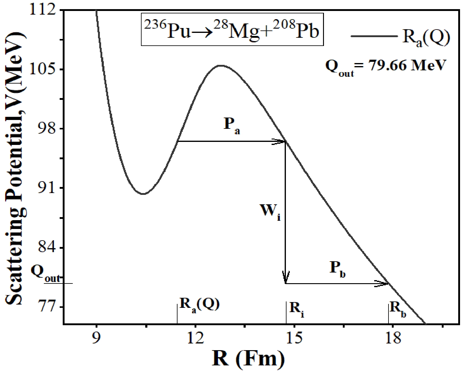
Figure 6. (color online) Scattering potential for the decay of
$ ^{236} $ Pu for cluster radioactivity using R$ _a $ (Q).The deformation parameters are taken from Ref. [54], and
$ R_{0i} $ can be written as$ \begin{equation} R_{0i}=[1.28A_{i}^{{1}/{3}}-0.76+0.8A_{i}] ~ {\rm fm}, \end{equation} $

(11) where i = 1, 2 are the radii of the fragments, and
$ \beta_{\lambda i} $ is taken to be zero for spherical choice of nuclei. Furthermore,$ \Delta R $ is the relative separation distance between two fragments or clusters$ A_i $ and is supposed to assimilate the neck formation effects. Hence, it is referred to as the neck length parameter [26]. The decay half-life$ T_{1/2} $ and decay constant λ are calculated as$ \begin{equation} T_{1/2}=\frac{{\rm ln} 2}{\lambda},\quad \lambda=\nu_o P_0P. \end{equation} $

(12) Here,
$ \nu_o $ is the barrier assault frequency, calculated as$ \begin{equation} \nu_o=\frac{\rm velocity}{R_0}=\frac{(2E_2/\mu)^{1/2}}{R_0}, \end{equation} $

(13) where
$ R_0 $ is the radius of the parent nucleus, μ is the reduced mass, and$ E_2 $ , the kinetic energy related to the Q-value, is given as$ E_2=(A_1/A)Q $ . -
This section represents the theoretical investigation of different ground state decay mechanisms (α, CR, HPR, and SF) using the PCM for nuclei with Z = 89−102. First, in Sec. III.A, the Q-value dependent first turning point
$ R_a $ (Q) is obtained, and an alpha decay analysis of the chosen set of isotopes is conducted using this relation. The overall trends of the preformation probability ($ P_o $ ) and penetrability (P) are analyzed as functions of the mass of the parent or daughter nucleus. In Secs. III.B and III.C, the decay half-lives are estimated in reference to CR and HPR using$ R_a $ (Q) of the respective mode, and a comparison is made with the available literature. Finally, an SF analysis is conducted for the chosen set of nuclei in Sec. III.D. -
In this section, an alpha decay analysis of the heavy mass region (Z = 89−102, A = 207−258) is carried out using the PCM. As discussed earlier, the nuclei in this mass range are highly radioactive, and alpha decay is the prominent decay mode in general [57, 58]. Therefore, it will be interesting to explore the alpha decay mechanism and study its behavior with respect to an increase in the mass or neutron number of the parent nucleus. α disintegration from a radioactive parent nucleus is the emission of a stable α nucleus along with a complementary daughter. The shell closure effects associated with the parent or daughter nucleus are the main reason for radioactive disintegration. The final product of radioactive disintegration is basically the decaying fragments associated with nearby proton or neutron shell closure. Hence, shell effects significantly affect alpha decay or other radioactive decay mechanisms (CR, HPR, and SF), and the associated decay constant or decay half-life is influenced accordingly.
As a first step, the α decay half-lives of actinium isotopes (
$^{207}{\rm Ac}$ ,$^{209}{\rm Ac}$ ,$^{211}{\rm Ac}$ ,$^{213}{\rm Ac}$ ,$^{215}{\rm Ac}$ ,$^{217}{\rm Ac}$ , and$^{221}{\rm Ac}$ ) are calculated using the PCM. Calculations are performed using the optimum choice of the neck length parameter ($ \Delta R $ ). In reference to available data, a comparison between the calculated and experimental half-lives [59] is conducted and shown in Fig. 1(a). The calculated half-lives are in good agreement with the experimental data. It may be noted from the figure that the decay half-life for N = 128 (with daughter nucleus$ {N}_2 =$ 126) is the shortest among the isotopes. Hence, nuclei with$ N_2 =$ 126 are more stable due to the neutron shell closure effect. After the calculation of the decay half-lives, the Q-value of the decay channel, i.e., Q$ _\alpha $ , is plotted with respect to the neutron number$ N_2 $ of the daughter nucleus, as shown in Fig. 1(b). Note that$ Q_\alpha $ has the highest magnitude for the nucleus with N = 128 ($ N_2 $ = 126) compared with its neighboring nuclei. As a result,$ Q_\alpha $ also demonstrates the significance of shell closure effects. As mentioned earlier, the PCM operates in terms of the mass asymmetry coordinate (η) and relative separation coordinate (R). Similarly, in a prior investigation of the PCM [60], it was found that the relative separation R and neck length parameter (ΔR) play key roles in the determination of different decay properties associated with radioactive nuclei.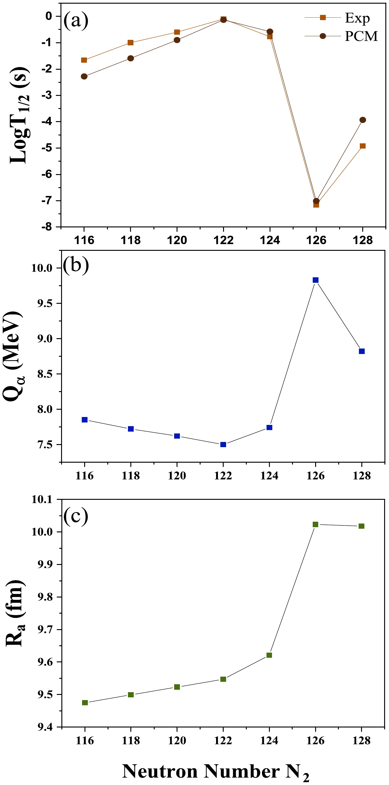
Figure 1. (color online) Variation in the (a) PCM calculated logarithmic half-lives for α decay and experimental data, as a function of neutron number (N
$ _2 $ ) of the daughter nucleus, (b) Q-value for alpha decay, (c) variation in the first turning point$ R_a $ (=$ R_1 $ +$ R_2 $ +$ \Delta R $ ).The calculations of the preformation probability and barrier penetrability are carried out at the first turning point R
$ _a $ , which is the sum of$ R_t $ and ΔR, i.e., R$ _a $ =R$ _t $ +$ \Delta R $ . Hence, to observe the role of the first turning point, the$ R_a $ point is plotted as a function of the neutron number$ N_2 $ of the daughter nucleus, as shown in Fig. 1(c). It may be noted that$ R_a $ has the highest magnitude at$ N_2 $ =126, in accordance with Q$ _\alpha $ and the decay half-life effect. This motivates us to obtain a Q-value dependent$ R_a $ relation, i.e.,$ R_a $ (Q). Therefore, to construct$ R_a $ (Q), two ranges of nuclei, Z = 89−93 and Z = 94−102, are chosen and a graph is made between the ratio ($ R_a $ /$ R_t $ ) against Q$ _\alpha $ , as shown in Fig. 2(a) and (b), where$ R_t $ is the sum of the radii$ R_1 $ and$ R_2 $ . The$ R_a $ points here are calculated by fitting the decay half-lives with respect to the available experimental data [59, 61]. Hence, using Fig. 2(a) and (b), we can obtain the polynomials$ R_a $ (Q) for the two ranges of nuclei.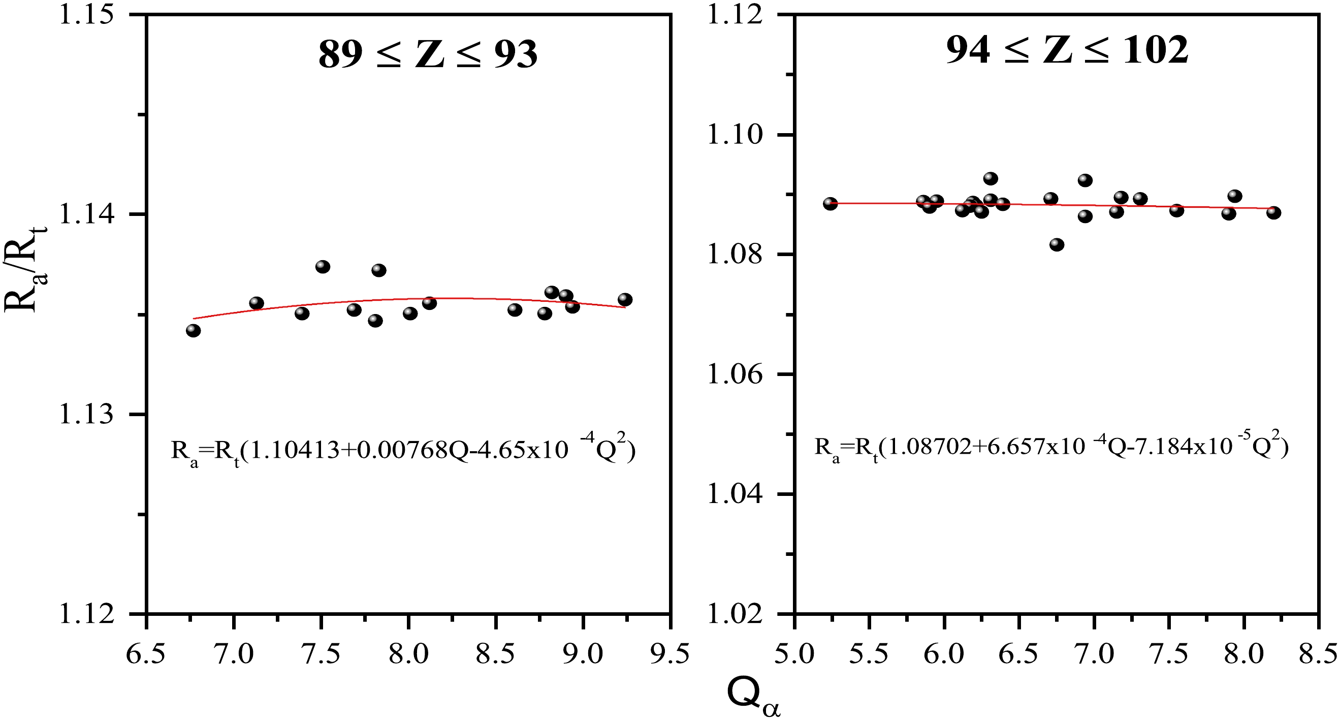
Figure 2. (color online) Variation in
$ R_a/R_t $ with respect to Q$ _\alpha $ for the chosen set of nuclei (a) Z = 89−93, (b) Z = 94−102, where the fitted polynomial is represented by the solid line.$ \begin{equation} {R_a}(Q)={R_t}(A_{1}+A_{2}Q_\alpha-A_{3}Q^2_{\alpha}) \quad 89\le Z \le93 ,\end{equation} $

(14) $ \begin{equation} {R_a}(Q)={R_t}(B_1+B_{2}Q_\alpha-B_{3}Q^2_{\alpha}) \quad 94\le Z \le102. \end{equation} $

(15) Here,
$ A_1 $ =1.10413,$ A_2 $ =0.00768, and$ A_3 $ =4.65x$ 10^{-4} $ , and similar constants for heavier nuclei are$ B_1 $ =1.08702,$ B_2 $ =6.657x$ 10^{-4} $ , and$ B_3 $ =7.184x$ 10^{-5} $ . Hence, we may use Eqs. (14) and (15) to calculate the$ R_a $ point for lighter and heavier nuclei, respectively. Validation of the above$ R_a $ (Q) relations (Eqs. (14) and (15) is performed by calculating the alpha decay half-lives of the same set of lighter and heavier nuclei. A comparison of both types of$ R_a $ points, i.e., R$ _a(\Delta R) $ and$ R_a(Q) $ , is shown in Table 1. A comparison of the calculated decay half lives is shown with the available experimental data.Parent nucleus Decay channel Ra(ΔR)
/fmRa(Q)
/fmlogT1/2[Ra(fm)(ΔR)]
/seclogT1/2[Ra(Q)]
/seclogT1/2/s
(Exp.)Z = 89−93 $ ^{212} $ Ac

$ ^{4} $ He+

$ ^{208} $ Fr

9.73 9.89 0.00 −0.03 −0.02 $ ^{219} $ Ac

$ ^{4} $ He+

$ ^{215} $ Fr

10.01 10.01 −3.93 −3.93 −4.92 $ ^{222} $ Ac

$ ^{4} $ He+

$ ^{218} $ Fr

10.05 10.02 2.28 2.23 0.73 $ ^{213} $ Th

$ ^{4} $ He+

$ ^{209} $ Ra

9.94 9.91 −0.80 −0.84 −0.85 $ ^{220} $ Th

$ ^{4} $ He+

$ ^{216} $ Ra

10.02 10.02 −4.91 −4.91 −5.01 $ ^{222} $ Th

$ ^{4} $ He+

$ ^{218} $ Ra

10.05 10.03 −2.11 −2.12 −2.55 $ ^{221} $ Pa

$ ^{4} $ He+

$ ^{217} $ Ac

10.04 10.05 −4.99 −5.00 −5.23 $ ^{224} $ Pa

$ ^{4} $ He+

$ ^{220} $ Ac

10.07 10.05 1.03 1.00 −0.10 $ ^{225} $ Pa

$ ^{4} $ He+

$ ^{221} $ Ac

10.08 10.06 1.07 1.03 0.38 $ ^{223} $ U

$ ^{4} $ He+

$ ^{219} $ Th

10.06 10.06 −2.78 −2.78 −4.74 $ ^{224} $ U

$ ^{4} $ He+

$ ^{220} $ Th

10.07 10.07 −3.44 −3.44 −3.05 $ ^{225} $ U

$ ^{4} $ He+

$ ^{221} $ Th

10.08 10.07 0.24 0.21 −1.00 $ ^{225} $ Np

$ ^{4} $ He+

$ ^{221} $ Pa

10.08 10.08 −3.20 −3.21 $> $ -5.7

$ ^{227} $ Np

$ ^{4} $ He+

$ ^{223} $ Pa

10.11 10.09 −0.15 −0.14 −0.29 $ ^{230} $ Np

$ ^{4} $ He+

$ ^{226} $ Pa

10.14 10.12 5.22 5.24 $ \le $ 3.96

Z = 94−102 $ ^{228} $ Pu

$ ^{4} $ He+

$ ^{224} $ U

9.72 9.70 −0.01 0.16 −0.70 $ ^{230} $ Pu

$ ^{4} $ He+

$ ^{226} $ U

9.74 9.73 2.75 2.80 $ \ge $ 2.30

$ ^{232} $ Pu

$ ^{4} $ He+

$ ^{228} $ U

9.76 9.75 4.85 4.88 4.20 $ ^{234} $ Pu

$ ^{4} $ He+

$ ^{230} $ U

9.78 9.78 6.71 6.74 5.72 $ ^{235} $ Pu

$ ^{4} $ He+

$ ^{231} $ U

9.80 9.79 8.91 8.91 7.75 $ ^{236} $ Pu

$ ^{4} $ He+

$ ^{232} $ U

9.81 9.80 8.93 8.93 8.11 $ ^{239} $ Pu

$ ^{4} $ He+

$ ^{235} $ U

9.84 9.84 12.63 12.63 12.00 $ ^{232} $ Am

$ ^{4} $ He+

$ ^{228} $ Np

9.76 9.75 3.72 3.77 3.59 $ ^{237} $ Am

$ ^{4} $ He+

$ ^{233} $ Np

9.82 9.82 7.70 7.70 7.18 $ ^{240} $ Cm

$ ^{4} $ He+

$ ^{236} $ Pu

9.85 9.85 7.24 7.24 6.52 $ ^{242} $ Cm

$ ^{4} $ He+

$ ^{238} $ Pu

9.87 9.88 8.40 8.41 7.28 $ ^{243} $ Cm

$ ^{4} $ He+

$ ^{239} $ Pu

9.88 9.89 9.21 9.21 8.96 $ ^{244} $ Cm

$ ^{4} $ He+

$ ^{240} $ Pu

9.89 9.90 9.89 9.89 8.88 $ ^{250} $ Cf

$ ^{4} $ He+

$ ^{246} $ Cm

9.96 9.97 9.87 9.87 8.69 $ ^{252} $ Cf

$ ^{4} $ He+

$ ^{248} $ Cm

9.98 9.99 9.71 9.71 8.00 $ ^{251} $ Es

$ ^{4} $ He+

$ ^{247} $ Bk

10.02 9.98 9.33 9.32 7.48 $ ^{253} $ Es

$ ^{4} $ He+

$ ^{249} $ Bk

9.94 10.00 7.73 7.63 6.30 $ ^{254} $ Es

$ ^{4} $ He+

$ ^{250} $ Bk

10.05 10.01 9.12 9.13 7.38 $ ^{250} $ Fm

$ ^{4} $ He+

$ ^{246} $ Cf

9.96 9.97 3.96 3.90 $< $ 3.30

$ ^{252} $ Fm

$ ^{4} $ He+

$ ^{248} $ Cf

9.98 9.99 5.73 5.71 5.04 $ ^{255} $ Md

$ ^{4} $ He+

$ ^{251} $ Es

10.01 10.02 3.28 3.24 3.21 $ ^{260} $ Md

$ ^{4} $ He+

$ ^{256} $ Es

10.06 10.08 8.64 8.62 $> $ 6.98

$ ^{254} $ No

$ ^{4} $ He+

$ ^{250} $ Fm

10.00 10.01 2.28 2.28 1.86 To observe the relevance of the polynomials in Eqs. (14) and (15), in the context of alpha decay within the PCM, the standard rms deviation is calculated using the equation
$ \begin{equation} \sigma = \sqrt{\sum{[{\rm log}_{10}({T_i}/{T_{{\rm expt}.}})]^2}/{n-1}} \, , \end{equation} $

(16) where n is the total number of parent nuclei under consideration. The standard deviation of the decay half-lives using Eqs. (14) and (15) is 1.14 and 1.05, respectively, whereas we obtain 1.15 and 1.05 for the optimized
$ \Delta R $ values, respectively. Furthermore, the scattering potential of$ ^{236} $ Pu is plotted with respect to the internuclear separation distance R by taking the$ R_a $ point from the Q dependent relation (Eq. (15)) and that shown in Fig. 3. We also compare the R$ _a $ point by taking the optimum choice of$ \Delta R $ and obtain a similar result. Hence, we may use these Q-dependent relations to calculate the decay half-lives of radioactive nuclei because they provide a good approximation to experimental data. After this, an investigation of several nuclei is carried out from Z = 82−93 and Z = 94−102, and a comparison is conducted between the half-lives calculated using$ {R}_a $ (Q) and the experimental values, as shown in Table 2 and Table 3. As shown in these tables, the$ R_a $ (Q) calculated decay half-lives are in good agreement with the experimental data, except for a few cases. The difference between the experimental alpha decay half-lives and the calculated values may arise in the case of certain nuclei, particularly neutron-deficient and neutron-rich isotopes. These isotopes may exhibit deviations from the predicted decay half-lives owing to specific nuclear structure effects and underlying physics. Moreover, these results are compared with the observations of other theoretical models, i.e., the ASAFM [62] and effective liquid drop model (ELDM) [63], which further reveals a reasonable agreement. Hence, Eqs. (14) and (15) can be used to calculate the decay half-lives of radioactive nuclei. After calculating the decay half-lives, the overall trend of the Q-value, penetration probability, preformation probability, and decay half-lives is studied, where all of these values are calculated using the$ R_a $ (Q) relation. In Fig. 4(a), the calculated Q$ _\alpha $ using the$R_a({Q})$ relation is plotted against the neutron number of the parent nuclei. At N = 128 ($ N_2= $ 126), Q$ _\alpha $ is maximum owing to the shell closure effects of the daughter nucleus. Such nuclei are relatively unstable; therefore, they have higher Q-values and the decay rate is relatively fast. Furthermore, as one approaches from N = 126 to N = 142, i.e., away from the shell closure, Q$ _\alpha $ starts decreasing, and this trend is compared with Fig. 1(a) of Ref. [64], which is shown in the inset of Fig. 4 (a). Moreover, in Fig. 4(b), Q$ _\alpha $ decreases sharply around A = 217−235. This is due to the effect of the neutron shell closure of the daughter nuclei for A = 217−219 (N = 128,$ N_2 $ = 126). It begins to decrease as we move away from the shell closure. Note that there are few stable nuclei (against alpha decay) at mass number A$ \ge $ 230 (here, the q-value is approximately 4 MeV, and the respective half-life is very large, that is,$ \; $ 10$ ^{19} $ ). Beyond this, Q$ _\alpha $ starts increasing, which may be due to the presence of the next shell closure after$ N_2= $ 126.Parent nucleus Decay channel Qα
/MeVRa/fm
(Poly.)logT1/2/s
(Poly.)logT1/2/s
ASAFM [62]logT1/2/s
ELDM [63]logT1/2/s
(Exp) [59]$ ^{207} $ Ac

$ ^{4} $ He+

$ ^{203} $ Fr

7.84 9.82 −3.62 3.30 −1.60 −1.66 $ ^{208} $ Ac

$ ^{4} $ He+

$ ^{204} $ Fr

7.72 9.84 −1.18 4.50 −1.16 −1.02 $ ^{209} $ Ac

$ ^{4} $ He+

$ ^{205} $ Fr

7.72 9.85 −2.78 − −1.18 −1.00 $ ^{210} $ Ac

$ ^{4} $ He+

$ ^{206} $ Fr

7.60 9.86 −0.41 − −0.80 −0.44 $ ^{211} $ Ac

$ ^{4} $ He+

$ ^{207} $ Fr

7.62 9.88 −2.06 − −0.88 −0.60 $ ^{213} $ Ac

$ ^{4} $ He+

$ ^{209} $ Fr

7.49 9.90 −1.15 − −0.48 −0.10 $ ^{215} $ Ac

$ ^{4} $ He+

$ ^{211} $ Fr

7.74 9.93 −1.33 − −1.36 −0.77 $ ^{217} $ Ac

$ ^{4} $ He+

$ ^{213} $ Fr

9.83 10.02 −6.94 −6.90 −6.99 −7.16 $ ^{218} $ Ac

$ ^{4} $ He+

$ ^{214} $ Fr

9.37 10.02 −4.19 −6.50 −5.96 −7.16 $ ^{210} $ Th

$ ^{4} $ He+

$ ^{206} $ Ra

8.06 10.01 −3.91 − −1.85 −5.96 $ ^{212} $ Th

$ ^{4} $ He+

$ ^{208} $ Ra

7.95 9.89 −3.41 −1.20 −1.57 −1.52 $ ^{214} $ Th

$ ^{4} $ He+

$ ^{210} $ Ra

7.82 9.92 −2.10 −0.80 −1.19 −1.00 $ ^{216} $ Th

$ ^{4} $ He+

$ ^{212} $ Ra

8.07 9.95 −2.73 −1.50 −2.00 −1.55 $ ^{218} $ Th

$ ^{4} $ He+

$ ^{214} $ Ra

9.85 10.03 −7.37 − −6.71 −6.96 $ ^{219} $ Th

$ ^{4} $ He+

$ ^{215} $ Ra

9.51 10.03 −4.66 −5.96 − −5.96 $ ^{224} $ Th

$ ^{4} $ He+

$ ^{220} $ Ra

7.29 10.05 1.08 0.00 0.43 0.11 $ ^{226} $ Th

$ ^{4} $ He+

$ ^{222} $ Ra

6.45 10.07 4.85 3.30 3.79 3.38 $ ^{228} $ Th

$ ^{4} $ He+

$ ^{224} $ Ra

5.52 10.12 9.53 7.90 8.38 7.92 $ ^{230} $ Th

$ ^{4} $ He+

$ ^{226} $ Np

4.76 10.17 14.13 12.50 13.05 12.49 $ ^{232} $ Th

$ ^{4} $ He+

$ ^{228} $ Ra

4.08 10.22 19.41 − 18.45 17.76 $ ^{213} $ Pa

$ ^{4} $ He+

$ ^{209} $ Ac

8.39 9.92 −4.22 − −2.53 −2.28 $ ^{214} $ Pa

$ ^{4} $ He+

$ ^{210} $ Ac

8.27 9.93 −2.04 − −2.19 $ \ge $ −1.77

$ ^{215} $ Pa

$ ^{4} $ He+

$ ^{211} $ Ac

8.24 9.94 −3.48 −1.80 −2.12 −1.82 $ ^{216} $ Pa

$ ^{4} $ He+

$ ^{212} $ Ac

8.09 9.95 −1.36 1.30 −1.68 −0.54 $ ^{217} $ Pa

$ ^{4} $ He+

$ ^{213} $ Ac

8.48 9.97 −3.43 −2.30 −2.89 −2.47 $ ^{218} $ Pa

$ ^{4} $ He+

$ ^{214} $ Ac

9.80 10.03 −5.32 −3.70 −6.25 −3.74 $ ^{219} $ Pa

$ ^{4} $ He+

$ ^{215} $ Ac

10.09 10.06 −7.59 −6.90 −6.92 −7.28 $ ^{220} $ Pa

$ ^{4} $ He+

$ ^{216} $ Ac

9.65 10.05 −4.65 −5.50 −6.37 −6.11 $ ^{227} $ Pa

$ ^{4} $ He+

$ ^{223} $ Ac

6.58 10.09 4.67 3.70 3.68 3.73 $ ^{218} $ U

$ ^{4} $ He+

$ ^{214} $ Th

8.77 9.99 −4.54 − −3.35 −2.82 $ ^{222} $ U

$ ^{4} $ He+

$ ^{218} $ Th

9.43 10.07 −5.97 − −5.27 −6.00 $ ^{226} $ U

$ ^{4} $ He+

$ ^{222} $ Th

7.70 10.08 −0.02 −0.30 −0.21 −0.70 $ ^{228} $ U

$ ^{4} $ He+

$ ^{224} $ Th

6.80 10.10 3.73 2.90 3.17 $< $ 2.76

$ ^{229} $ U

$ ^{4} $ He+

$ ^{225} $ Th

6.47 10.11 6.34 4.30 4.57 4.43 $ ^{230} $ U

$ ^{4} $ He+

$ ^{226} $ Th

5.99 10.13 7.83 6.40 6.85 6.43 $ ^{233} $ U

$ ^{4} $ He+

$ ^{229} $ Th

4.90 10.20 14.63 12.70 13.18 12.77 $ ^{226} $ Np

$ ^{4} $ He+

$ ^{222} $ Pa

8.19 10.08 0.03 − −1.37 −1.15 $ ^{228} $ Np

$ ^{4} $ He+

$ ^{224} $ Pa

7.30 10.10 2.86 − 1.23 2.18 $ ^{229} $ Np

$ ^{4} $ He+

$ ^{225} $ Pa

7.01 10.11 3.38 2.30 2.78 $< $ 2.66

$ ^{231} $ Np

$ ^{4} $ He+

$ ^{227} $ Pa

6.36 10.14 6.45 5.40 5.52 5.18 Table 2. PCM-calculated alpha decay half-lives LogT
$ _{1/2} $ of 31 nuclei for Z = 89−93. Using Eq. (14), the results are compared with the available experimental data.Parent nucleus Decay channel Qα
/MeVRa/fm
(Poly.)logT1/2/s
(Poly.)logT1/2/s
ASAFM [62]logT1/2/s
ELDM [63]logT1/2/s
(Exp.) [59]$ ^{233} $ Pu

$ ^{4} $ He+

$ ^{229} $ U

6.41 9.77 7.00 5.80 5.72 6.00 $ ^{238} $ Pu

$ ^{4} $ He+

$ ^{234} $ U

5.59 9.83 10.73 9.50 9.88 9.59 $ ^{240} $ Pu

$ ^{4} $ He+

$ ^{236} $ U

5.25 9.85 12.42 11.40 11.88 11.45 $ ^{242} $ Pu

$ ^{4} $ He+

$ ^{238} $ U

4.98 9.88 14.08 − 13.64 13.18 $ ^{238} $ Cm

$ ^{4} $ He+

$ ^{234} $ Pu

6.67 9.83 5.63 4.90 5.64 $ \ge $ 4.93

$ ^{246} $ Cm

$ ^{4} $ He+

$ ^{242} $ Pu

5.47 9.92 12.34 − 11.50 11.26 $ ^{248} $ Cm

$ ^{4} $ He+

$ ^{244} $ Pu

5.16 9.95 14.48 − 13.46 13.15 $ ^{250} $ Cm

$ ^{4} $ He+

$ ^{246} $ Pu

5.16 9.97 14.68 − 13.38 12.45 $ ^{240} $ Cf

$ ^{4} $ He+

$ ^{236} $ Cm

7.71 9.85 2.30 − 2.00 1.81 $ ^{242} $ Cf

$ ^{4} $ He+

$ ^{238} $ Cm

7.51 9.87 3.24 2.40 2.70 2.41 $ ^{244} $ Cf

$ ^{4} $ He+

$ ^{240} $ Cm

7.32 9.90 3.96 3.10 3.43 3.18 $ ^{246} $ Cf

$ ^{4} $ He+

$ ^{242} $ Cm

6.86 9.92 5.97 − 5.34 5.20 $ ^{248} $ Cf

$ ^{4} $ He+

$ ^{244} $ Cm

6.36 9.95 8.52 − 7.63 7.54 $ ^{251} $ Cf

$ ^{4} $ He+

$ ^{247} $ Cm

6.17 9.98 10.68 10.90 8.52 10.45 $ ^{254} $ Cf

$ ^{4} $ He+

$ ^{250} $ Cm

5.92 10.02 11.27 9.30 9.79 9.30 $ ^{256} $ Cf

$ ^{4} $ He+

$ ^{252} $ Cm

5.56 10.04 13.48 − 11.90 10.87 $ ^{252} $ Es

$ ^{4} $ He+

$ ^{248} $ Bk

6.78 9.99 9.67 7.60 5.99 7.61 $ ^{245} $ Fm

$ ^{4} $ He+

$ ^{241} $ Cf

8.43 9.99 1.73 − 0.28 0.62 $ ^{246} $ Fm

$ ^{4} $ He+

$ ^{242} $ Cf

8.37 9.91 0.80 − 0.50 0.08 $ ^{248} $ Fm

$ ^{4} $ He+

$ ^{244} $ Cf

7.99 9.94 2.16 − 1.70 1.65 $ ^{254} $ Fm

$ ^{4} $ He+

$ ^{250} $ Cf

7.30 10.01 5.61 4.10 4.22 4.15 $ ^{256} $ Fm

$ ^{4} $ He+

$ ^{252} $ Cf

7.02 10.04 6.79 5.10 5.36 5.15 $ ^{247} $ Md

$ ^{4} $ He+

$ ^{243} $ Es

8.76 9.92 −0.10 − −0.86 0.46 $ ^{256} $ Md

$ ^{4} $ He+

$ ^{252} $ Es

7.73 10.03 5.28 3.90 2.36 3.66 $ ^{257} $ Md

$ ^{4} $ He+

$ ^{253} $ Es

7.55 10.05 5.02 3.70 3.60 4.30 $ ^{258} $ Md

$ ^{4} $ He+

$ ^{254} $ Es

7.27 10.06 7.96 5.80 4.73 6.65 $ ^{259} $ Md

$ ^{4} $ He+

$ ^{255} $ Es

7.10 10.07 7.10 − 5.39 $> $ 5.28

$ ^{250} $ No

$ ^{4} $ He+

$ ^{246} $ Fm

8.94 9.96 −0.32 − −0.65 −0.30 $ ^{252} $ No

$ ^{4} $ He+

$ ^{248} $ Fm

8.54 9.98 1.00 − 0.58 0.62 $ ^{255} $ No

$ ^{4} $ He+

$ ^{251} $ Fm

8.42 10.02 1.33 2.80 0.88 2.27 $ ^{256} $ No

$ ^{4} $ He+

$ ^{252} $ Fm

8.58 10.03 1.58 0.50 0.41 0.56 $ ^{258} $ No

$ ^{4} $ He+

$ ^{254} $ Fm

8.14 10.05 3.10 1.70 1.83 2.08 Table 3. PCM-calculated alpha decay half-lives LogT
$ _{1/2} $ of 32 nuclei for Z = 94−102. Using Eq. (15) the results are compared with the available experimental data.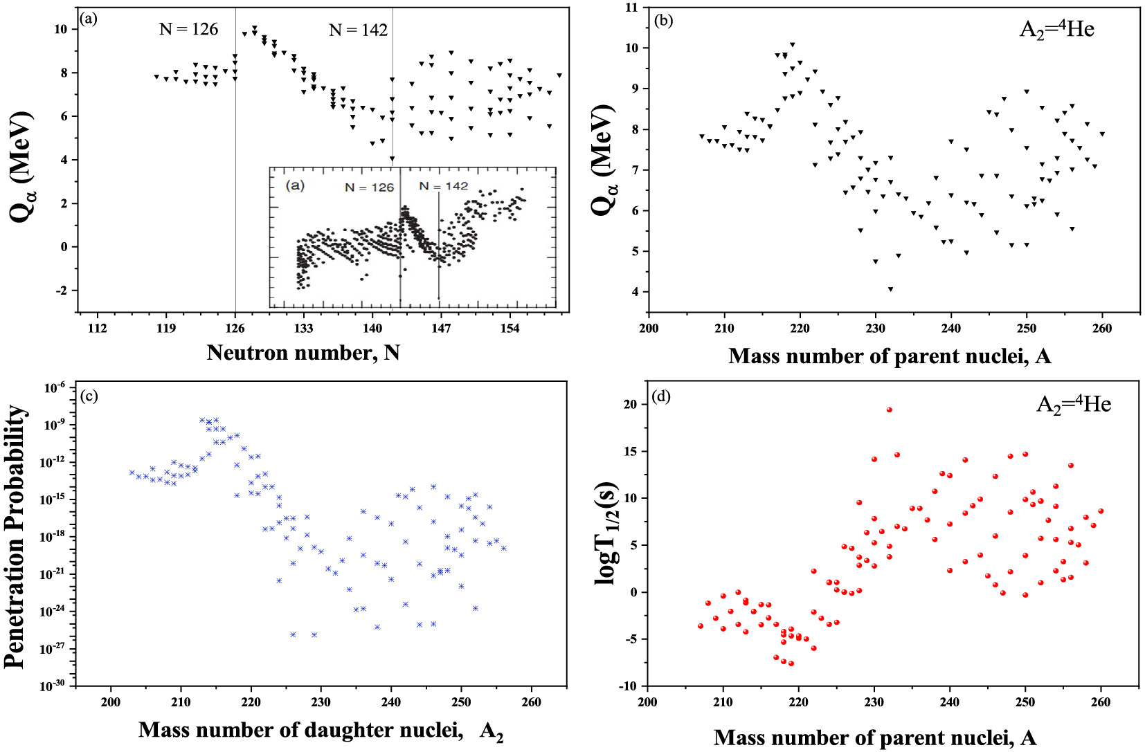
Figure 4. (color online) (a) Calculated Q
$ _\alpha $ as a function of the neutron number of the parent nucleus, the inset of the figure is taken from Ref. [64]. The scales of the x axis and y-axis represent the same quantities for both the graphs (i.e., Q$ _\alpha $ and neutron number (N)) of the parent nucleus. (b) Calculated Q$ _\alpha $ as a function of mass number, (c) penetration probability P as a function of A$ _2 $ , and (d) decay decay half-lives (logT1/2) as a function of A. All the above values are calculated for α decay data using R$ _a $ (Q) relations (Eqs. (14) and (15)).The penetration probability P is calculated and shown in Fig. 4(c). The penetration probability (the three step process is explained in Eq. (6)) and role of Q
$ _\alpha $ in penetrability can be visualized from Fig. 3. The penetration probability is maximum for$ {A_2}= $ 213−215 ($ {N_2}= $ 126); therefore, it is easier for the alpha particle to escape across these daughter nuclei. This is due to the neutron shell closure at N = 126. After the analysis of$ Q_\alpha $ and the penetrability, the PCM calculated alpha decay half-lives are plotted with respect to mass number A in Fig. 4(d). The decay half-lives depend on the decay constant, which further depend on the assault frequency (nearly constant), penetration probability, and preformation probability. Here, the penetration probability starts decreasing until A = 217 and then sharply increases between A = 217−235 because of the influence of shell effects, as mentioned earlier. In the next step, the preformation probability of the nuclei is calculated using Eqs. (14) and (15) and shown in Fig. 5. From this figure, we find that the preformation factor decreases with an increase in the mass number of the parent nuclei. In this study, the calculations are performed using collective clusterization, which treats all decay processes (such as α, cluster, heavy mass fragment, and fission decay) on equal footing. Therefore, the preformation probabilities of all binary fragments are obtained by solving the Schrödinger equation in the mass asymmetry coordinate η. Because the preformation probability is calculated in preview of the collective clusterization process, P$ _0 $ of one decay channel is affected by the relative contribution of the remaining fragments in the binary exit channel. Hence, alpha preformation is affected by other competing decay modes. A similar analysis of preformation probability using the GLDM for α decay is presented in Ref. [65].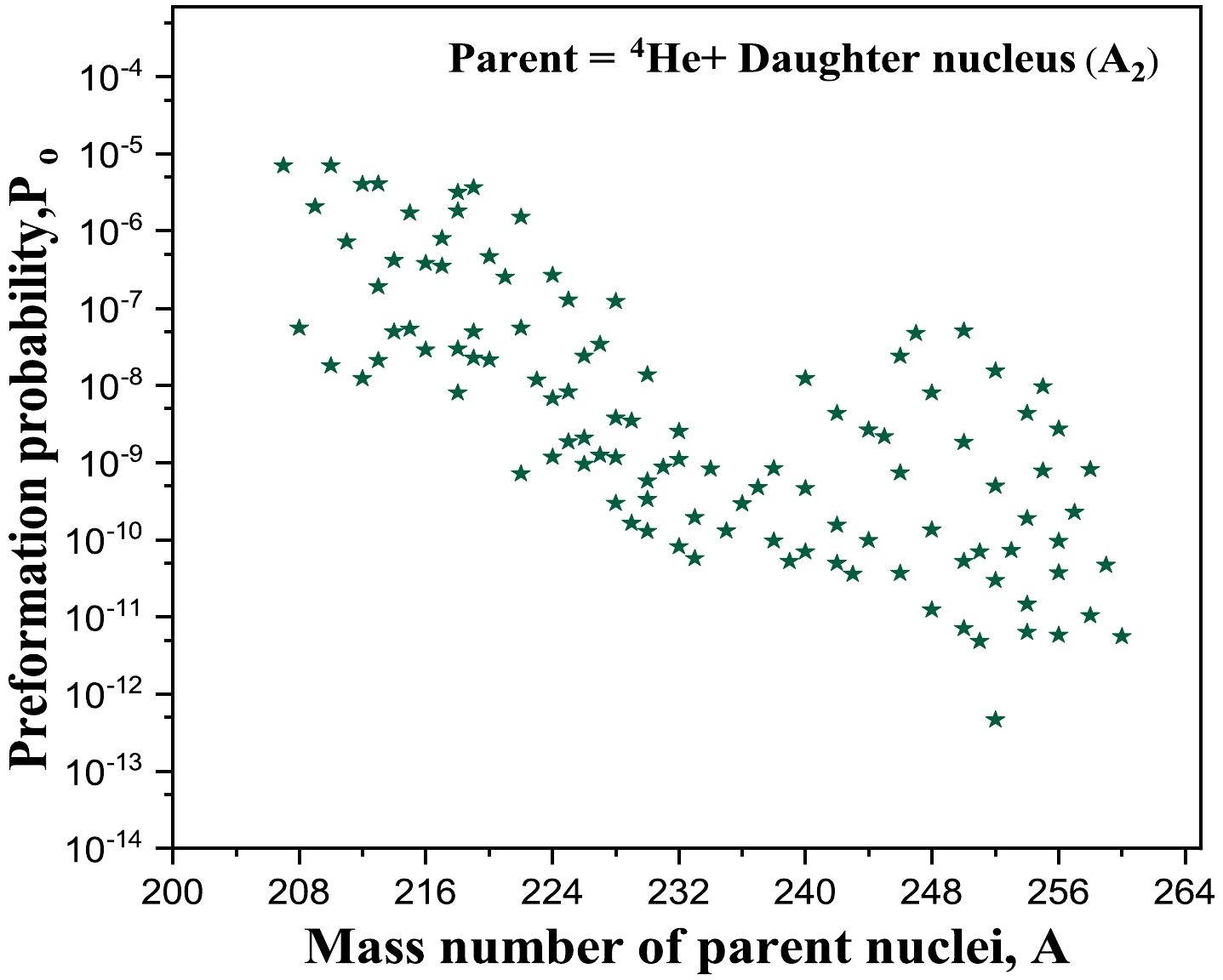
Figure 5. (color online) PCM calculated α preformation probability for 109 nuclei (Z = 89−102) as a function of the mass number of the parent nucleus.
-
In the previous section, alpha decay of different nuclei is investigated using the
$ R_a $ (Q) relation, and the calculated half-lives are found to be in good agreement with the available data. In the present section, the cluster emission is studied for the chosen set of isotopes using the$ R_a $ (Q) relation. Previously, in Refs. [66, 67], cluster decay analysis was performed using older mass tables or proximity potentials within the framework of the PCM. It is important to mention that the current calculations are performed using the mass table of Audi et al. 2017 [49]. The decay half-lives are calculated for the experimentally observed clusters via the optimization of the neck length parameter$ \Delta R $ , and the appropriate value of the R$ {_a} $ point is fixed. The obtained R$ {_a} $ value is further used to get the R$ {_a} $ (Q) relation for the spherical and deformed choice of the decaying fragments using the same procedure as mentioned in the previous section for the α decay case. The R$ {_a} $ (Q) relations for the CR process read as$ \begin{equation} {R_a}(Q)={R_t}({C_1-C_2Q_{\rm cluster}+C_3Q^2_{\rm cluster}}), \end{equation} $

(17) $ \begin{equation} {R_a}(Q)= {R_t}({D_1-D_2Q_{\rm cluster}+D_3Q^2_{\rm cluster}}), \end{equation} $

(18) where Eq. (17) is for the spherical choice of the decaying fragments, and Eq. (18) is for the deformed choice of the decaying fragments. Q
$_{\rm cluster}$ is the q-value of the decay channel. In Eq. (17),$ C_1 $ =1.05502,$ C_2 $ =1.17016×10$ ^{-4} $ , and$ C_3 $ =3.424×$ 10^{-7} $ . Similarly, the constants for Eq. (18) are$ D_1 $ =1.0573,$ D_2 $ =2.07598×$ 10^{-4} $ , and$ D_3 $ =8.8151×$ 10^{-7} $ . Eqs. (17) and (18) can be employed to give the decay half-lives in a cluster decay mechanism. The validity of these equations can be tested via the comparison of the$ R_a $ (Q) calculated results with the corresponding experimental data. The comparison of the$ R_a $ (Q) calculated decay half-lives and the experimental results for the spherical and deformed choice of the decaying fragments is shown in Table 4. In this table,$ R_a $ is obtained using the$ R_a $ (Q) relation. It may be noted from the table that the calculated$ R_a $ points and corresponding decay half-lives are in good agreement with experimental data. We find that the deformed choice of the decaying fragment offers relatively better agreement with the experimental data compared to the spherical case. In addition, to check the validity of the polynomials used, the standard deviation (SD) is calculated with respect to the experimental results. For the spherical choice of the decaying fragments, the SDs are 4.20 and 4.21 for$ R_a $ and$ R_a $ (Q), respectively. An SD of more than 3 with data is considered not good. Hence, the spherical clusters do not impart good agreement. After analyzing the spherical choice, the SDs are calculated for the deformed choice of clusters, which are 2.75 and 2.77 for$ R_a $ and$ R_a $ (Q), respectively. Furthermore, the calculated half-lives are compared with the data of theoretical models, i.e., the ASAFM [62] and mean-field approximation in the Hartree-Fock-Bogoliubov (HFB) [40], which shows a reasonable agreement with the predicted data. Similar to the alpha decay analysis, a scattering plot for the CR of$ ^{236} $ Pu is plotted with respect to internuclear separation distance (R) by taking the first turning point R$ _a $ from Eq.(18), as shown in Fig. 6. Then, the first turning point is compared by taking the optimum choice of$ \Delta R $ .Parent nucleus Decay channel Q $_{\rm cluster}$ 

/MeVPCM Spherical Deformed ASAFM
log$ T_{1/2} $ /s

HFB
log$ T_{1/2} $ /s

[62]Expt.
log$ T_{1/2} $ /s

[40]$ R_a $ /fm

(Poly.)logT $_{1/2}/{\rm s}$ 

(Poly.)$ R_a $ /fm

(Poly.)logT $ _{1/2} $ /s

(Poly.)$ ^{223} $ Ac

$ ^{14} $ C +

$ ^{209} $ Bi

33.06 10.12 17.06 10.16 14.77 12.7 − 12.60 $ ^{223} $ Ac

$ ^{15} $ N +

$ ^{208} $ Pb

39.47 10.17 18.85 10.17 16.91 14.1 − $> $ 14.76

$ ^{225} $ Ac

$ ^{14} $ C +

$ ^{211} $ Bi

30.47 10.15 21.54 10.19 20.77 17.8 − 17.16 $ ^{226} $ Th

$ ^{14} $ C +

$ ^{212} $ Po

30.54 10.16 22.29 10.18 21.26 17.7 − $> $ 15.3

$ ^{226} $ Th

$ ^{18} $ O +

$ ^{208} $ Pb

45.72 10.35 22.43 10.37 21.70 18.0 17.31 $> $ 15.3

$ ^{228} $ Th

$ ^{20} $ O +

$ ^{208} $ Pb

44.72 10.47 23.54 10.48 22.79 21.9 19.53 20.87 $ ^{230} $ Th

$ ^{24} $ Ne +

$ ^{206} $ Hg

57.76 10.64 26.90 10.70 25.96 25.2 25.08 24.61 $ ^{231} $ Pa

$ ^{23} $ F +

$ ^{208} $ Pb

51.88 10.62 25.25 10.86 24.29 25.9 − 26.02 $ ^{231} $ Pa

$ ^{24} $ Ne +

$ ^{207} $ Tl

60.40 10.65 23.37 10.71 22.65 23.3 − 23.23 $ ^{230} $ U

$ ^{22} $ Ne +

$ ^{208} $ Pb

61.38 10.56 23.90 11.22 20.70 20.4 20.49 19.57 $ ^{230} $ U

$ ^{24} $ Ne +

$ ^{206} $ Pb

61.81 10.64 23.09 10.69 22.28 22.4 − $> $ 18.2

$ ^{232} $ U

$ ^{24} $ Ne +

$ ^{208} $ Pb

62.30 10.66 21.09 10.72 20.28 20.8 23.35 21.05 $ ^{232} $ U

$ ^{28} $ Mg +

$ ^{204} $ Hg

74.31 10.79 26.01 11.52 21.91 − − $> $ 22.26

$ ^{233} $ U

$ ^{24} $ Ne +

$ ^{209} $ Pb

60.48 10.68 25.77 10.76 24.76 25.2 − 24.84 $ ^{233} $ U

$ ^{25} $ Ne +

$ ^{208} $ Pb

60.70 10.71 25.08 10.82 24.15 25.7 − 24.84 $ ^{233} $ U

$ ^{28} $ Mg +

$ ^{205} $ Hg

74.22 10.81 27.50 11.42 24.26 27.4 − $> $ 27.59

$ ^{234} $ U

$ ^{24} $ Ne +

$ ^{210} $ Pb

58.82 10.69 28.26 10.74 27.14 26.1 27.24 25.92 $ ^{234} $ U

$ ^{25} $ Ne +

$ ^{209} $ Pb

57.79 10.73 29.49 10.86 28.31 28.8 − 25.92 $ ^{234} $ U

$ ^{26} $ Ne +

$ ^{208} $ Pb

59.41 10.76 26.39 11.02 24.93 27.0 28.02 25.92 $ ^{234} $ U

$ ^{28} $ Mg +

$ ^{206} $ Hg

74.11 10.82 26.81 11.42 23.35 25.9 25.85 25.54 $ ^{235} $ U

$ ^{24} $ Ne +

$ ^{211} $ Pb

57.36 10.70 32.16 10.76 30.24 − − 27.62 $ ^{235} $ U

$ ^{25} $ Mg +

$ ^{210} $ Pb

57.68 10.74 45.97 10.84 29.20 − − 27.62 $ ^{235} $ U

$ ^{28} $ Mg +

$ ^{207} $ Hg

72.42 10.83 30.66 11.46 26.32 − − $> $ 28.09

$ ^{235} $ U

$ ^{29} $ Mg +

$ ^{206} $ Hg

72.46 10.86 30.38 11.37 26.61 − − $> $ 28.09

$ ^{236} $ U

$ ^{28} $ Mg +

$ ^{208} $ Hg

70.73 10.85 32.37 11.45 28.45 − 33.68 27.58 $ ^{236} $ U

$ ^{30} $ Mg +

$ ^{206} $ Hg

72.27 10.91 28.78 11.17 26.46 29.8 33.1 27.58 $ ^{238} $ U

$ ^{34} $ Si +

$ ^{204} $ Pt

85.18 11.04 30.63 11.02 29.85 − − 29.04 $ ^{237} $ Np

$ ^{30} $ Mg +

$ ^{207} $ Tl

74.79 10.92 26.41 11.18 23.88 28.3 − $> $ 26.93

$ ^{236} $ Pu

$ ^{28} $ Mg +

$ ^{208} $ Pb

79.66 10.84 20.36 11.45 16.19 21.1 20.13 21.67 $ ^{238} $ Pu

$ ^{28} $ Mg +

$ ^{210} $ Pb

75.91 10.87 26.94 11.48 22.65 26.2 29.42 25.70 $ ^{238} $ Pu

$ ^{30} $ Mg +

$ ^{208} $ Pb

76.79 10.93 24.48 11.19 22.02 26.2 29.52 25.70 $ ^{238} $ Pu

$ ^{32} $ Si +

$ ^{206} $ Hg

91.18 10.98 25.25 11.12 22.84 26.1 28.23 25.27 $ ^{240} $ Pu

$ ^{34} $ Si +

$ ^{206} $ Hg

91.02 11.06 24.57 11.05 22.73 27.4 26.96 $> $ 25.52

$ ^{241} $ Am

$ ^{34} $ Si +

$ ^{207} $ Tl

93.92 11.07 21.80 11.06 20.16 25.8 − $> $ 22.71

$ ^{242} $ Cm

$ ^{34} $ Si +

$ ^{208} $ Pb

96.50 11.08 19.44 11.07 17.98 23.5 24.9 23.24 $ ^{252} $ Cf

$ ^{46} $ Ar +

$ ^{206} $ Hg

126.75 11.48 16.41 11.66 14.98 26.5 − $> $ 15.89

$ ^{252} $ Cf

$ ^{48} $ Ca +

$ ^{204} $ Pt

138.17 11.52 18.61 11.52 18.27 − − $> $ 15.89

$ ^{252} $ Cf

$ ^{50} $ Ca +

$ ^{202} $ Pt

138.31 11.56 17.73 11.71 15.95 − − $> $ 15.89

Table 4. Comparison of decay half-lives of various experimentally detected clusters with those calculated using prox 1977 with in the PCM for spherical and deformed choices of nuclei. The corresponding Q
$_{\rm cluster}$ are calculated using the binding energies of Audi et al. [49] given for each decay.This comparison give similar results. Therefore, it is clear from the above calculations that the SD is reduced for the deformed choice of fragments. Therefore, the polynomial in Eq. (18) gives a reasonable approximation and can be used to calculate the decay half-lives of other sets of nuclei belonging to the heavy/superheavy region.
-
Following the analysis of the α and cluster decays, HPR is studied in this section. In a previous study [4, 6], one of us and collaborators predicted the decay half-lives of the heavy clusters emitted by certain heavy nuclei. In this study, we extend the previous work to the full range of actinide series. The HPR results are shown in Table 5. Here, the most probable HPR fragments are identified using the minima in the fragmentation potential. The calculated Q-values of the decay channel, i.e.,
$Q_{\rm HPR}$ , and the decay half-lives are also shown in Table 5.$ R_a $ (Q) for the HPR case is given asParent nucleus Decay channel Q $_{\rm HPR}$ /MeV

R $ _a $ (Poly.)

log $ T_{1/2} $ /s Poly.

$ ^{232} $ U

$ ^{82} $ Ge+

$ ^{150} $ Nd

173.70 10.92 30.32 $ ^{234} $ U

$ ^{82} $ Ge+

$ ^{152} $ Nd

173.71 10.95 30.54 $ ^{236} $ U

$ ^{82} $ Ge+

$ ^{154} $ Nd

173.68 10.98 29.40 $ ^{238} $ U

$ ^{82} $ Ge+

$ ^{156} $ Nd

173.19 11.01 30.07 $ ^{240} $ Pu

$ ^{82} $ Ge+

$ ^{158} $ Sm

180.79 11.04 28.07 $ ^{242} $ Pu

$ ^{82} $ Ge+

$ ^{160} $ Sm

180.36 11.07 28.19 $ ^{244} $ Pu

$ ^{82} $ Ge+

$ ^{162} $ Sm

179.75 11.10 28.32 $ ^{246} $ Pu

$ ^{82} $ Ge+

$ ^{164} $ Sm

178.90 11.12 28.93 $ ^{238} $ Cm

$ ^{84} $ Se+

$ ^{154} $ Sm

198.75 11.03 23.05 $ ^{240} $ Cm

$ ^{84} $ Se+

$ ^{156} $ Sm

197.03 11.05 24.00 $ ^{242} $ Cm

$ ^{84} $ Se+

$ ^{158} $ Sm

196.00 11.08 25.27 $ ^{244} $ Cm

$ ^{82} $ Ge+

$ ^{162} $ Gd

188.14 11.10 25.85 $ ^{246} $ Cm

$ ^{82} $ Ge+

$ ^{164} $ Gd

187.80 11.12 26.06 $ ^{248} $ Cm

$ ^{82} $ Ge+

$ ^{166} $ Gd

187.33 11.15 25.93 $ ^{250} $ Cm

$ ^{82} $ Ge+

$ ^{168} $ Gd

186.76 11.18 26.37 $ ^{244} $ Cf

$ ^{84} $ Se+

$ ^{160} $ Gd

205.36 11.11 21.37 $ ^{246} $ Cf

$ ^{84} $ Se+

$ ^{162} $ Bk

204.30 11.14 22.26 $ ^{248} $ Cf

$ ^{84} $ Se+

$ ^{164} $ Gd

202.95 11.17 23.55 $ ^{250} $ Cf

$ ^{82} $ Ge+

$ ^{168} $ Dy

195.14 11.18 24.07 $ ^{252} $ Cf

$ ^{82} $ Ge+

$ ^{170} $ Dy

195.10 11.20 23.68 $ ^{254} $ Cf

$ ^{82} $ Ge+

$ ^{172} $ Dy

194.76 11.23 22.71 Table 5. PCM calculated half-lives for the heavy particle radioactivity of Z=89−102 parent systems. The choice of the outgoing fragment is based on the most probable fragment with the highest preformation probability. Note that in each case, the spherical choice of fragments is considered, and calculations with
$ l=0 \hbar $ and$ T=0 $ MeV with only the optimized$ \Delta R $ as −0.25 is set of all isotopes.$ \begin{equation} {R_a}= R_t(E_1+E_{2}Q_{\rm HPR}-E_{3}Q^2_{\rm HPR}). \end{equation} $

(19) Here,
$ E_1 $ =0.9484,$ E_2 $ =3.055×10$ ^{-4} $ , and$ E_3 $ =7.867×$ 10^{-7} $ The calculations of the first turning point ($ R_a $ ) by taking the optimum value of the parameter$ \Delta R $ and using Eq. (19) are shown in Columns 4 and 5, respectively. The half lives are represented in the last two columns. The predicted fragments are isotopes of Ge because these nuclei exhibit shell effects around N = 50. These heavy clusters are not yet experimentally detected; therefore, it will be of future interest to verify the validity of such predictions. -
In the previous sections, an analysis of α emission, CR, and HPR is conducted using their respective
$ R_a $ (Q) relations. It is concluded that the first turning point plays a crucial role in exploring the dynamics of these decay modes. It is known that alpha decay and SF are the most observed decay modes. In this section, a comprehensive analysis is performed among the α decay and SF modes using the PCM. It is relevant to note that within the PCM approach, all the decay modes are explored on an equal footing. The most probable decaying fragments of a radioactive nucleus can be identified using the fragmentation structure and preformation probability. In Fig. 7, the fragmentation structure and preformation probability$ P_0 $ are compared for the$ ^{230} $ Th and$ ^{256} $ No nuclei (extreme nuclei of the chosen mass region). The trend of the fragmentation structure for the$ ^{230} $ Th and$ ^{256} $ No nuclei (see Fig. 7(a) and (c)) remains similar for both modes (α and SF), but changes in the magnitude of the fragmentation potential are observed. The minima in the fragmentation potential suggest the most probable decay fragments. The identified fission fragments using the minima of the fragmentation potential for alpha decay and SF for the$ ^{230} $ Th and$ ^{256} $ No nuclei are$ ^{96} $ Sr+$ ^{134} $ Te and$ ^{124} $ Sn+$ ^{132} $ Te, respectively. After the fragmentation structure, the preformation probability is calculated and plotted with respect to fragment mass$ A_i $ and shown in Fig. 7(b) and (d). The trend of the preformation probability is also similar for the$ ^{230} $ Th and$ ^{256} $ No nuclei in the α and SF decay modes. The fission region is found to change from the asymmetric to symmetric mode when going from the$ ^{230} $ Th to$ ^{256} $ No nucleus. It will be interesting to explore the transition point where the mass distribution changes from the asymmetric to symmetric mode.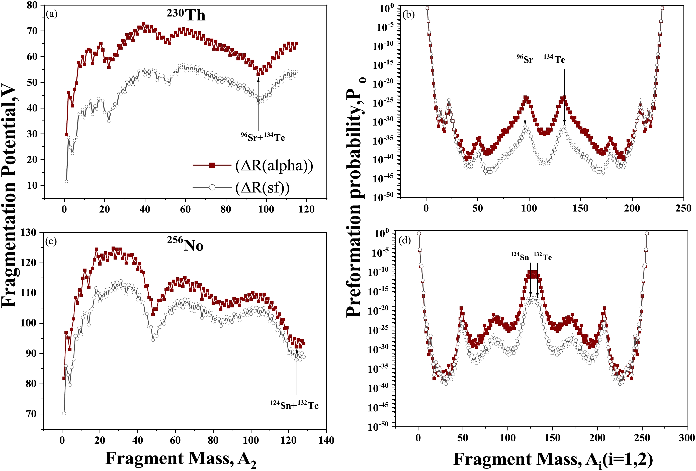
Figure 7. (color online) Fragmentation potential and preformation probability of nuclei for (a), (b)
$ ^{230} $ Th and (c), (d)$ ^{256} $ No for alpha and spontaneous fission by taking the emitting fragments as spheres only.To gain a better insight into this transition, we take two more isotopes (
$ ^{252} $ Cf and$ ^{256} $ Fm) from the chosen range of nuclei, and the preformation probability is plotted as a function of fragment mass$ A_i $ (i = 1, 2), as shown in Fig. 8. For the SF analysis, the decay half-lives are calculated for the$ ^{230} $ Th,$ ^{252} $ Cf,$ ^{256} $ Fm, and$ ^{256} $ No nuclei first for the spherical case. Then, the deformation effects are included up to quadrupole ($ \beta{_2} $ ) deformations with hot optimum orientations of the decay fragments. A comparison between the calculated decay half-lives and the experimental data [68] is shown in Table 6. The calculated results are in reasonable agreement with the experimental data, except for the spherical choice fragments for the$ ^{256} $ Fm nucleus because the calculated half-lives are found to underestimate the experimental SF data. It is relevant to note that the half-life increases with decreasing$ \Delta R $ value. However, in the case of$ ^{256} $ Fm,$ \Delta R $ cannot be reduced further as V(R$ _a $ ) becomes less than Q$ _{\rm sf} $ (Q-value of the decaying channel). On the other hand, we have a reasonable scope of the$ \Delta R $ extension for$ ^{256} $ No because the barrier characteristics become modified as Coulomb repulsion increases with increasing atomic number. Interestingly, the barrier height can be altered for the$ ^{256} $ Fm nucleus by adding deformations. The calculated half life of$ ^{256} $ Fm becomes modified by taking a hot-compact choice of fragments, as shown in Table 6.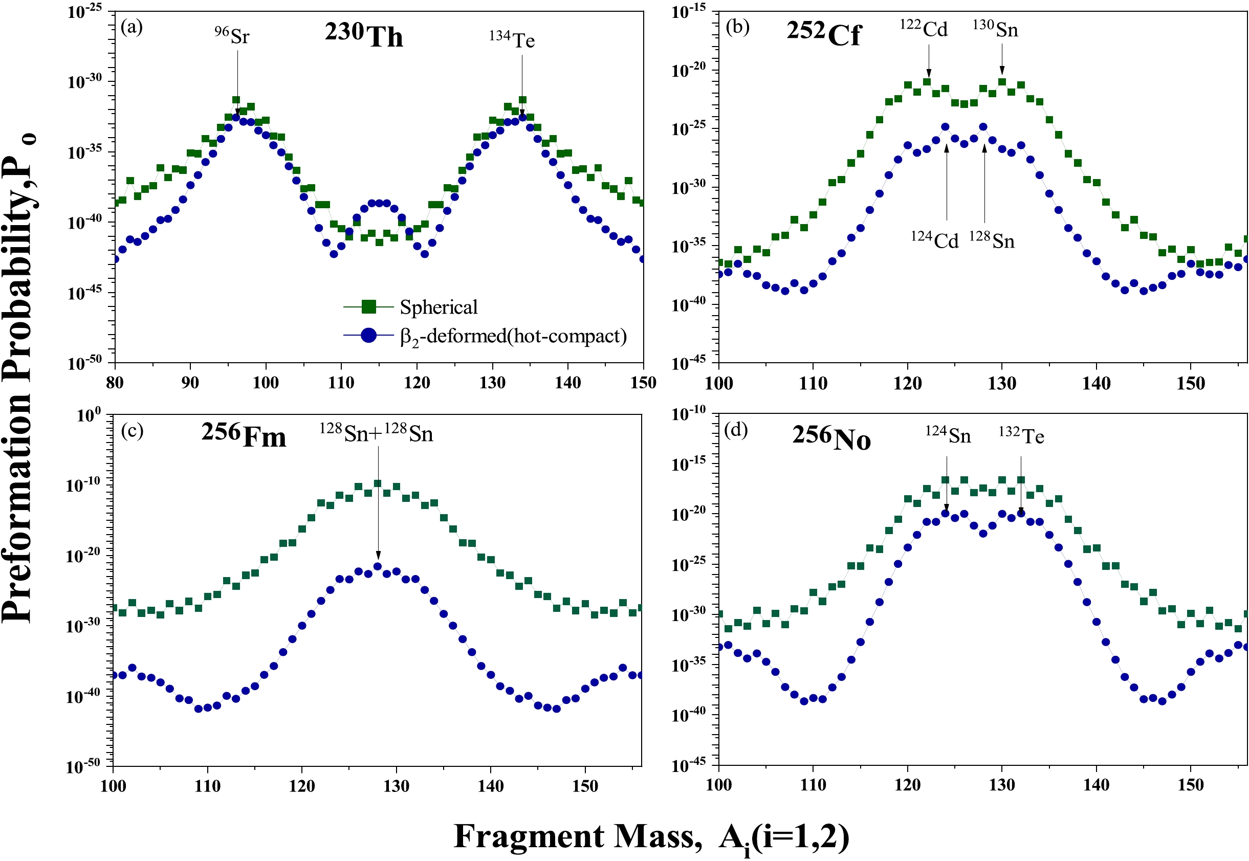
Figure 8. (color online) Preformation yield
$ P_o $ as a function of fission fragments (a)$ ^{230} $ Th, (b)$ ^{252} $ Cf, (c)$ ^{256} $ Fm, and (d)$ ^{256} $ No for spherical fragments as well as$ \beta_2 $ deformed hot compact configurations.Parent nucleus Decay channel $ R_a $ 

/fm${\rm log}_{10}T^{\rm SF}_{1/2}$ /s

(PCM)${\rm log}_{10}T^{\rm SF}_{1/2}$ /s

(Exp.)Spherical $ ^{230} $ Th

$ ^{96} $ Sr+

$ ^{134} $ Te

10.82 24.25 24.79 $ ^{252} $ Cf

$ ^{122} $ Cd+

$ ^{130} $ Sn

11.33 9.00 9.43 $ ^{256} $ Fm

$ ^{128} $ Sn+

$ ^{128} $ Sn

12.20 −7.36 4.01 $ ^{256} $ No

$ ^{124} $ Sn+

$ ^{132} $ Te

11.49 2.31 2.73 Deformed $ ^{230} $ Th

$ ^{96} $ Sr+

$ ^{134} $ Te

11.34 24.16 24.79 $ ^{252} $ Cf

$ ^{124} $ Cd+

$ ^{128} $ Sn

12.12 9.40 9.43 $ ^{256} $ Fm

$ ^{128} $ Sn+

$ ^{128} $ Sn

12.24 4.25 4.01 $ ^{256} $ No

$ ^{124} $ Sn+

$ ^{132} $ Te

12.37 2.09 2.73 Table 6. PCM-calculated half life for spontaneous fission along with the fitted neck-length parameter
$ \Delta R $ . The choice of the outgoing fragment is based on the most probable fragment with the highest preformation probability. Note that in each case, spherical as well as$ \beta_2 $ -deformed (hot) orientations are taken into consideration. The calculated half-lives are also compared with experimental data [68].The identified most probable fission fragments for spherical as well as a hot-compact choice of fragments are also shown in Table 6. For the
$ ^{230} $ Th nucleus, the asymmetric fission fragments$ ^{96} $ Sr+$ ^{134} $ Te (N = 82) are identified, which lie near N = 82 and the deformed magic number Z = 38. For the$ ^{252} $ Cf nucleus, asymmetric fragments ($ ^{122} $ Cd+$ ^{130} $ Sn) are identified, which lie near Z = 50. The symmetric fission fragments of$ ^{256} $ Fm also belong to the spherical magic shell closure Sn(Z=50) and near the neutron shell closure N = 82. Similarly, symmetric fragments of$ ^{256} $ No are identified near Z = 50. This indicates that proton and neutron shell closures play an important role in the SF region. These results are in fair agreement with Refs. [69, 70]. Furthermore, the SF half-life is calculated for a chosen set of nuclei Z$ \sim $ 89−102, whose experimental data are available. For these cases, the neck length parameter ($ \Delta R $ ) ranges from −0.5 to 0.8 fm. A comparison between the calculated half-life and experimental data is shown in Fig. 9. The calculated results show good agreement with experimental data [71−73].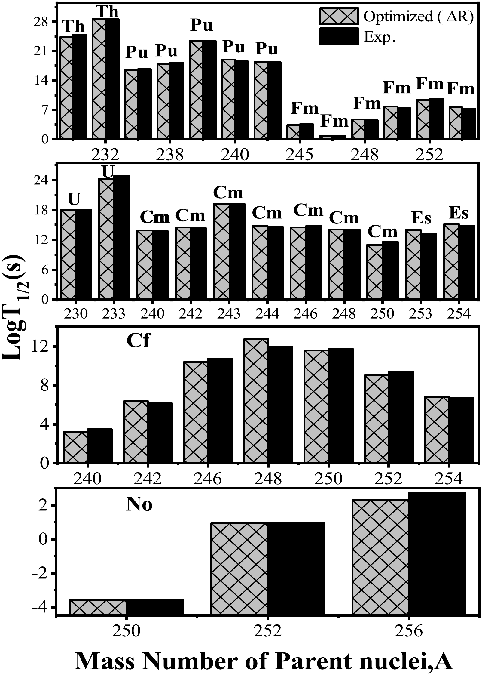
Figure 9. Logarithmic half-lives for 34 nuclei undergoing spontaneous fission in the range Z=89−102 compared with experimental half-lives by optimizing
$ \Delta R $ .In addition, the TKE is also studied for these nuclei because it plays an important role in SF dynamics. It alters its behavior with respect to the symmetry/asymmetry of the decaying fragments. The TKE can be computed using the relation taken from Herbach et al. [74] as follows:
$ \begin{equation} TKE = \frac{0.2904(Z_1+Z_2)^2}{A_1^{1/3}+A_2^{1/3}-(A_1+A_2)^{1/3}} \frac{A_1A_2}{(A_1+A_2)^2} ,\end{equation} $

(20) where
$ A_1 $ and$ A_2 $ are the mass numbers of the emitted fragments. First, the TKE is calculated for the nuclei whose experimental data are available, as shown in Table 7. Because the fragments appearing at the minima in Eq. (3) correspond to the most probable fragments, the calculated results are found to be in good agreement with experimental data. Second, experimental analyses of certain nuclei are not yet available for SF. Therefore, an attempt is made to predict the TKE for cases where experimental data are absent, as shown in Fig. 10. It is evident from this figure that the TKE of the fragments increases with an increase in the fissility parameter ($ Z^2 $ $/A ^{1/3} $ ). Because of an increase in the fissile nature of the nuclei, the mass of the decaying fragments increases, leading to an increase in the TKE values. It will be of future interest to compare the calculated TKE values with experimental data.Parent nucleus Decay channel TKE/MeV Calc. Expt. $ ^{238} $ Pu

$ ^{104} $ Mo+

$ ^{134} $ Te

174.26 177.00±0.5 $ ^{240} $ Pu

$ ^{106} $ Mo+

$ ^{134} $ Te

174.05 179.40±0.5 $ ^{242} $ Pu

$ ^{110} $ Ru+

$ ^{132} $ Sn

174.23 180.70±0.5 $ ^{246} $ Cm

$ ^{116} $ Pd+

$ ^{130} $ Sn

181.37 183.90±1.0 $ ^{248} $ Cm

$ ^{116} $ Pd+

$ ^{132} $ Sn

180.77 182.20±0.9, 179.00 $ \pm $ 2.0

$ ^{248} $ Cf

$ ^{120} $ Cd+

$ ^{128} $ Sn

188.79 188.70±1.3 $ ^{250} $ Cf

$ ^{120} $ Cd+

$ ^{130} $ Sn

188.21 187.00±1.0, 185.00 $ \pm $ 3.0

$ ^{252} $ Cf

$ ^{122} $ Cd+

$ ^{130} $ Sn

187.79 185.9±1.0, 185.70±0.1, 183.00±0.5 $ ^{254} $ Cf

$ ^{122} $ Cd+

$ ^{132} $ Sn

187.20 186.90±1.0, 185.00 $ \pm $ 2.0

$ ^{253} $ Es

$ ^{125} $ In+

$ ^{128} $ Sn

191.50 188.00±3.0 $ ^{254} $ Fm

$ ^{126} $ Sn+

$ ^{128} $ Sn

195.15 195.1±1.0, 189.00±2.0 $ ^{256} $ Fm

$ ^{126} $ Sn+

$ ^{130} $ Sn

194.65 197.9±1.0 $ ^{252} $ No

$ ^{122} $ Sn+

$ ^{130} $ Sn

203.43 202.4±0.0, 194.30±3.0 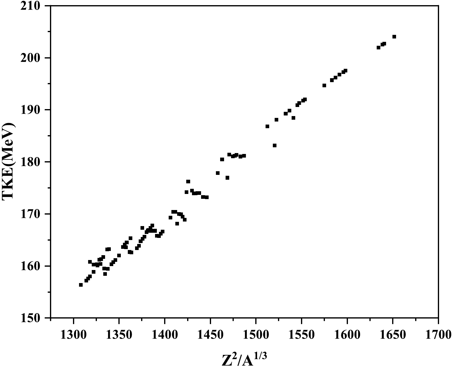
Figure 10. TKE vs
$ Z^{2}/A^{1/3} $ for 93 nuclei in the range Z = 89−102. -
In summary, the PCM is employed for the study of different ground state decay modes, such as α decay, CR, HPR, and SF, from nuclei in the range Z = 89−102. The α decay half-lives are calculated for two sets of chosen nuclei using the fitting neck length parameter (
$ \Delta R $ ). The obtained neck length parameter is further used to calculate the Q-value dependent first turning point, i.e., R$ _a $ (Q). The$ R_a $ (Q) relations are employed to calculate the α decay half-lives of other sets of nuclei within the chosen range, which are found to be in good agreement with experimental data. The overall analysis of the preformation probability (P$ _0 $ ) and penetration probability (P) for alpha decay is studied with respect to an increase in the mass number of the parent/daughter nucleus. The calculated preformation probability decreases with increasing mass number of the parent nuclei. This may be associated with the corresponding enhancement in$ P_o $ of the fissioning region. The role of the neutron shell closure at$ N_2= $ 126 is clearly visible from the trend of the penetration probability. After the alpha decay analysis, the$ R_a $ (Q) relations are obtained for the CR and HPR decay modes. In the case of CR, the$ R_a $ (Q) relation with the deformed choice gives better agreement with the experimental data compared to the spherical choice. Furthermore, a comparative analysis of α-decay and SF is conducted using the fragmentation potential and preformation distribution for extreme choices of nuclei ($ ^{230} $ Th and$ ^{256} $ No) in the range Z=89−102. The overall fragmentation structure remains the same for both decay modes, and the identified fission fragments are also similar. The mass distribution of the$ ^{230} $ Th and$ ^{256} $ No nuclei is studied, which is found to change from asymmetric to symmetric. An attempt is made to identify the transition from the asymmetric to symmetric distribution. To study the transition point, the mass distribution of$ ^{252} $ Cf and$ ^{256} $ fm along with extreme nuclei in the range Z = 89−102 ($ ^{230} $ Th and$ ^{256} $ No) is investigated. After the analysis of the fragmentation potential, probable fission fragments are identified. In addition, the TKE of these fission fragments is calculated and compared with experimental data, and predictions of the TKE are made for a chosen range of nuclei. As an extension of this study, it will be of further interest to compare the TKE of the most probable fission fragments for the spherical and deformed choices of decaying fragments.
Study of various ground state decay mechanisms of Actinide nuclei
- Received Date: 2023-05-29
- Available Online: 2023-10-15
Abstract: The special property of the actinide mass region is that nuclei belonging to this group are radioactive and undergo different ground state processes, such as alpha decay, cluster radioactivity (CR), heavy particle radioactivity (HPR), and spontaneous fission (SF). In this study, the probable radioactive decay modes of the heavy mass region (Z = 89−102) are studied within the framework of the preformed cluster model (PCM). In the PCM, the radioactive decay modes are explored in terms of the preformation probability (


 DownLoad: