


 Abstract
 HTML
HTML Reference
 Related
 PDF
PDF


-
To explain the observed cosmological matter-antimatter asymmetry, baryon number B violation is one of three basic ingredients for an initially symmetric universe [1]. The baryon number is necessarily violated in the Grand Unified Theories (GUTs) [2, 3], which can unify the strong, weak, and electromagnetic interactions into a single underlying force at a scale of
$M_{\rm{GUT}}\simeq 2 \times 10^{16}\; \rm{GeV}$ . A general prediction of the GUTs is proton decay. However, no experimental evidence of proton decay, B-violating neutron decay, or neutron-antineutron oscillation has been found [4]. Fortunately, a new generation of underground experiments, JUNO [5, 6], Hyper-Kamiokande [7], and DUNE [8], with large target masses and different detection technologies will continue to search for proton decay and test the GUTs.Among the many possible proton decay modes [4],
$ p\to e^+ \pi^0 $ and$ p\to \bar{\nu} K^+ $ are the two dominant modes predicted by most of the GUTs. The former is expected to be the leading mode in many GUTs, particularly in non-supersymmetric GUTs, which typically predict the lifetime of the proton to be approximately$ 10^{35} $ years [9]. In comparison, the decay mode$ p\to \bar{\nu} K^+ $ is favored by a number of supersymmetric GUTs. For these two decay modes, the best measured upper limits of proton partial lifetime are$ \tau/B(p \to e^+ \pi^0) > 2.4 \times 10^{34} $ years [10] and$\tau/B(p \to \bar{\nu} K^+) > 5.9 \times 10^{33}$ years [11] at the 90% C.L. from the Super-Kamiokande (Super-K) experiment, which uses a water Cherenkov detector.Compared to water Cherenkov detectors, liquid scintillator (LS) detectors have a distinct advantage in detecting the proton decay mode
$ p\to \bar{\nu} K^+ $ [5, 12–14]. In this study, we investigate the sensitivity of the future LS detector, JUNO. Here, the decay gives rise to a three-fold coincidence feature in time, which is usually composed of a prompt signal by the energy deposit of$ K^+ $ , a short-delayed signal ($ \tau=12.38 $ ns) by the energy deposit of the decay daughters of$ K^+ $ , and a long-delayed signal ($\tau=2.2$ μs) by the energy deposit of the final Michel electron. Using the time-correlated triple coincidence, the JUNO detector can effectively identify$ p\to \bar{\nu} K^+ $ and reject atmospheric neutrino backgrounds [14].Preliminary studies have given a rough estimate of the sensitivity of JUNO to the proton decay mode
$ p\to \bar{\nu} K^+ $ [5]. In this study, the JUNO potential based on a detailed detector performance analysis is investigated using Monte Carlo (MC) simulation. Sec. II briefly introduces the JUNO detector and its expected performance. In Sec. Ⅲ, MC simulation of$ p\to \bar{\nu} K^+ $ and the atmospheric ν backgrounds is described. In Sec. IV, the multi-pulse fitting method and other selection criteria to discriminate$ p\to \bar{\nu} K^+ $ from the backgrounds are investigated. We present the expected sensitivity of JUNO to$ p\to \bar{\nu} K^+ $ in Sec. V. Finally, a conclusion is given in Sec. VI. -
JUNO is a multi-purpose neutrino observatory under construction in South China. As a low background observatory, it has a vertical overburden of 700 m of rock (1800 m.w.e) to shield the detector from cosmic muons. Its central detector (CD) is a 12 cm thick acrylic sphere with a diameter of 35.4 m, containing a 20 kton LS. The CD is immersed in a cylindrical water pool and supported by a stainless steel lattice structure. Moreover, the CD is equipped with 17612 20-inch PMTs (LPMTs) and 25600 3-inch PMTs (SPMTs), which are uniformly distributed outside the acrylic sphere. 5000 LPMTs are dynode (DYN) PMTs produced by Hamamatsu Photonics K.K., whereas the remaining LPMTs are Micro Channel Plate (MCP) PMTs manufactured by North Night Vision Technology Co., Ltd. (NNVT) [15]. Their transit time spread (TTS) values are 1.1 ns and 5.0 ns, respectively, in σ according to the result of the PMT mass test [16]. The total photocathode coverage of the LPMT is around 75%. The SPMTs, which contribute another 2.5% of photocathode coverage, are also deployed to serve as an additional independent calorimeter. The TTS (σ) of the SPMTs has been measured to be approximately 1.5 ns [17]. For each MeV energy deposition in the LS when detecting low energy events, around
$ 1.3\times 10^{3} $ photonelectrons (PE) are expected to be received by the LPMTs.A VETO system, including a Top Tracker (TT) detector and water Cherenkov PMT system, is designed to prevent the influence of cosmic muons. A TT detector is a plastic scintillator detector complex that partly covers the water pool and CD, which helps reject the cosmic muons passing it. The water Cherenkov PMT system is assembled on the outer surface of the stainless steel lattice structure and measures the Cherenkov light produced by the cosmic muons passing the water pool. The rejection ratio of cosmic muons is estimated to be more than 99%.
-
To understand the behavior of
$ p\to \bar{\nu} K^+ $ and discriminate it from the backgrounds in the JUNO detector, an MC simulation is performed in two steps: generator production and detector simulation. The generator of$ p\to \bar{\nu} K^+ $ and its backgrounds is produced with GENIE (version 3.0.2) [18], in which the primary processes of$ p\to \bar{\nu} K^+ $ and the atmospheric ν interactions in the LS are simulated. The detector simulation, which is a simulation of the final states of$ p\to \bar{\nu} K^+ $ and the atmospheric ν interaction in the JUNO detector, is processed in SNiPER [19], which is a Geant4 [20] based simulation software developed by the JUNO collaboration. All related optical processes, including the quenching effect, are considered. The profiles of the LS, including the fluorescence times can be found in Ref. [21]. In total, 10 k$ p\to \bar{\nu} K^+ $ (PD) events and 160 k atmospheric ν events are simulated with vertex positions uniformly distributed over the entire LS volume.This study does not yet use full event reconstruction of energy, position, and hit time information. Instead, they are smeared according to the expectation from the detector MC simulation and used as the inputs for further analysis. The visible energy (
$ E_{\rm{vis}} $ ) is the energy deposition reconstructed from the number of PE received by the LPMTs. For a conservative consideration, it is smeared by 3%/$ {\sqrt{E_{\rm{vis}} ({\rm{MeV}})}} $ when the energy deposition is smaller than 60 MeV and by a resolution of 1% when greater [22]. The position of the event is described by the center of energy deposition position, which is the averaged position weighted by the energy deposition each time. It is smeared by a Gaussian distribution with a resolution of 30 cm. In this study, the detected times of photon hits on the cathode of the SPMT are collected to form a hit time spectrum for each event, after the correction of photon time-of-flight (TOF) relative to the reconstructed deposition center. The TTS of the SPMTs is set randomly according to the measurement results introduced in Sec. II. The reason for not using the LPMTs is introduced in Sec. III.A. -
Based on the JUNO LS components, the initial proton of
$ p\to \bar{\nu} K^+ $ may originate from free protons (in hydrogen) or bound protons (in carbon). In free proton decay, the final states$ \bar{\nu} $ and$ K^+ $ have fixed kinetic energies of 339 MeV and 105 MeV, respectively. According to a toy MC simulation with the corresponding monochromatic$ K^+ $ in the JUNO detector, it is found that 92.4% of$ K^+ $ will deposit all of their kinetic energy within 1.2 ns, which means a signal can be immediately found in the hit time spectrum. Then, these$ K^+ $ will stay at rest until decaying into their daughter particles after an average of 12.38 ns.$ K^+ $ has six main decay channels. The most dominant channels are$ K^+ \to \mu^+ \nu_\mu $ and$ K^+ \to \pi^+ \pi^0 $ , with branching ratios of 63.56% and 20.67%, respectively [4]. In the first channel, the produced$ \mu^+ $ has a kinetic energy of 152 MeV and decays into a Michel electron with a lifetime of approximately 2.2$\rm\mu s$ . The produced$ \pi^0 $ and$ \pi^+ $ in the second channel will decay into two gammas, a$ \mu^+ $ and a$ \nu_\mu $ , respectively, and consequently produce a Michel electron. All daughter particles will deposit their kinetic energies immediately and give a second signal. After the TOF correction, the hit time spectrum of$ K^{+} $ and the decay particles will form an overlapping double-pulse pattern. Given the relatively long lifetime of the muon, a later third pulse from the Michel electron, as a delayed feature of$ p\to \bar{\nu} K^+ $ , will be found on the hit time spectrum. This triple coincidence, as introduced in Sec. I, is one of the most important features for distinguishing a$ p\to \bar{\nu} K^+ $ event from the backgrounds. This triple coincidence is illustrated in Fig. 1.
Figure 1. (color online) Illustration of the hit time spectrum of a typical
$ p\to \bar{\nu} K^+ $ event, containing the signals of$ K^+ $ , the decay daughter of$ K^+ $ ($ \mu^{+} $ in this event), and the Michel electron.As introduced in Sec. II, both the LPMTs and SPMTs are used in JUNO. However, as shown in Fig. 2, they have different performances in hit time spectrum collection. When an LPMT is triggered by a hit, the waveform will be digitized and recorded by the electronics. Then, hit time reconstruction (from the waveform to the hit time of each PE) will be performed to obtain the hit time spectrum. For low energy events such as inverse β decay (IBD), hit time reconstruction is possible because only a few photons can be received by most LPMTs. However, a typical
$ p\to \bar{\nu} K^+ $ event usually has an energy deposition of more than 200 MeV. In this case, many PEs would be received by the LPMTs in a few tens of ns (as shown in Fig. 2(a)), and hit time reconstruction would be difficult. As shown in Fig. 2(b), the overlapping of the first two pulses of the triple coincidence time feature would be smeared if hit time reconstruction is not performed. Thus, the LPMTs are not used to collect the hit time spectrum in this study. In comparison, considering that the receiving area of the SPMTs is around 1/40 times that of the LPMTs, most SPMTs will work in single hit mode in which the SPMTs are usually hit by a maximum of one PE. Advantageously, the triple coincidence time feature of$ p\to \bar{\nu} K^+ $ can be well preserved. Thus, only the SPMTs in single hit mode are used in this study to collect the hit time spectrum.
Figure 2. (color online) Simulated PMT output of a typical
$ p\to \bar{\nu} K^+ $ event. The total visible energy of this event is 275 MeV, and$ K^+ $ decay occurs 13.7 ns after this. Photon hit time reconstruction is not easy to achieve when using LPMTs to detect a hundreds-of-MeV event. Therefore, an SPMT is used for hit time spectrum collection. More details can be found in the text.The protons bound in carbon nuclei are influenced by nuclear effects [11], including the nuclear binding energy, Fermi motion, and nucleon-nucleon correlation. The kinetic energies of the produced
$ K^+ $ are smeared around 105 MeV, which is relative to that in the free proton case. In addition, the$ K^+ $ kinetic energy is also changed by final state interactions (FSIs). Before the$ K^+ $ escapes from the residual nucleus, it may interact with spectator nucleons and knock one of them out of the remaining nucleus. It can also exchange its charge with a neutron and turn into$ K^0 $ via$ K^+ + n \to K^0 +p $ . Furthermore, the de-excitation of the residual nucleus will produce γ, neutrons, or protons, etc. Obviously, FSIs and de-excitation processes will change the reaction products, which are crucial to a later analysis.The GENIE generator (version 3.0.2) [18] is used to model these nuclear effects. Some corrections are made to the default GENIE. First, the nuclear shell structure is considered, which is not included in the default nuclear model of GENIE. A spectral function model, which provides a two-dimensional distribution of momentum k and the removal energy
$ E_R $ for protons in$ ^{12} {\rm{C}} $ , is applied to describe the initial proton states [23]. Then, the initial proton energy is determined by$ E_p = m_p - E_R $ , where$ m_p $ is the mass of a free proton. In this case, approximately 2.2% of the protons from$ ^{12} {\rm{C}} $ cannot decay into$ \bar{\nu} $ and$ K^+ $ because the corresponding proton invariant mass is smaller than the$ K^+ $ mass [24].Second, we turn on the hadron-nucleon model in GENIE. The default GENIE uses the hadron-atom model to evaluate the FSIs, which takes less time but does not include the
$ K^+ + n \to K^0 +p $ interaction. Meanwhile, we modify the target nucleon energy and binding energy with$ m_p - E_R $ (or$ m_n - E_R $ ) and$ E_B = E_R - k^2/(2 M_{^{11}\rm{B}}) $ [25], respectively. In addition, the fraction of$ K^+ $ -nucleon charge exchange and elastic scattering interactions is corrected in terms of the numbers of spectator protons and neutrons in the remaining nucleus. With all these modifications, we finally obtain a distribution of the$ K^+ $ kinetic energies, as shown in Fig. 3. The charge exchange probability is approximately 1.7% for$ p\to \bar{\nu} K^+ $ in$ ^{12} $ C according to the results of the modified GENIE.
Figure 3. (color online)
$ K^+ $ kinetic energy distributions for$ p\to \bar{\nu} K^+ $ in 12C with (solid line) and without (dashed line) the FSIs from the default (blue) and modified (red) GENIE.Third, all residual nuclei in the default GENIE are generated in the ground state; thus, no de-excitation processes are considered. The TALYS (version 1.95) software [26] is then applied to estimate the de-excitation processes due to the excitation energy
$ E_x $ .$ E_x $ of the residual nucleus can be calculated through$E_x = M_{\rm inv}-M_R$ , where$M_{\rm inv}$ and$ M_R $ are the corresponding invariant and static masses, respectively. For$ p\to \bar{\nu} K^+ $ in$ ^{12} {\rm{C}} $ ,$ ^{11} {\rm{B^*}} $ ,$ ^{10} {\rm{B^*}} $ , and$ ^{10} {\rm{Be^*}} $ account for 90.9%, 5.1%, and 3.1% of the residual nuclei, respectively. Among these residual nuclei,$ ^{10} {\rm{B^*}} $ and$ ^{10} {\rm{Be^*}} $ originate from the final state interactions between$ K^+ $ and one of the nucleons in$ ^{11} {\rm{B^*}} $ . The de-excitation modes and corresponding branching ratios of the residual nuclei$ ^{11} {\rm{B^*}} $ ,$ ^{10} {\rm{B^*}} $ , and$ ^{10} {\rm{Be^*}} $ have been reported in Ref. [24].According to the results, many de-excitation processes can produce neutrons. In the case of
$ s_{1/2} $ proton decay, the dominant de-excitation modes of the$ ^{11} {\rm{B^*}} $ states, including$ n + {^{10} {\rm{B}}} $ ,$ n + p + {^{9} {\rm{Be}}} $ ,$ n + d + {^{8} {\rm{Be}}} $ ,$ n + \alpha + {^{6} {\rm{Li}}} $ , and$ 2n +p + {^{8} {\rm{Be}}} $ , will contribute to a branching ratio of 45.8% [24]. Approximately 56.5% of highly excited$ ^{11} {\rm{B^*}} $ states can directly emit one or more neutrons from their exclusive de-excitation modes. In addition, non-exclusive de-excitation processes and the de-excitation modes of$ d + {^{9} {\rm{Be}}} $ and$ d + \alpha + {^{5} {\rm{He}}} $ can also produce neutrons [24]. Most of these neutrons give a 2.2 MeV γ from neutron capture in the JUNO LS, which influences the setting of the criteria (introduced in Section. IV.B). -
The dominant backgrounds of
$ p\to \bar{\nu} K^+ $ are caused by atmospheric ν and cosmic muons because the deposited energy of$ p\to \bar{\nu} K^+ $ events are usually larger than 100 MeV. Cosmic muons originate from the interaction between cosmic rays and the atmosphere. The produced cosmic muons usually have a very high energy and produce obvious Cherenkov light when passing through the water pool outside the JUNO CD. With the VETO system, JUNO is expected to discriminate more than 99% of cosmic muons. The muons not detected by the VETO system usually clip the corner of the water pool with a very low energy deposited and few Cherenkov photons produced and therefore escape from the watch of the VETO system. Thus, most VETO survived cosmic muons leave no signal in the CD and will not be background for$ p\to \bar{\nu} K^+ $ observations. For the muons that are VETO survived, producing entering and leaving signals in the CD, the energy deposition processes are mainly caused by the energetic primary muon. Consequently, with the visible energy, VETO, and volume selection, as well as the expected triple coincidence feature selection, this type of background is considered negligible. Therefore, the main background discussed in this paper arises from atmospheric ν events.The expected number of observed atmospheric ν events is calculated with the help of the atmospheric ν fluxes at the JUNO site [27], the neutrino cross sections from GENIE [18], and the best-fit values of the oscillation parameters in the case of the normal hierarchy [4]. The JUNO LS detector will observe 36 k events over ten years. We use GENIE in its default configuration to generate 160 k atmospheric ν events, which corresponds to 44.5 years of JUNO data collection or 890 kton-years exposure mass. Each atmospheric ν event has a weight value, which indicates the possibility of this event occurring for JUNO's 200 kton-years exposure considering neutrino oscillation. Then, these atmospheric ν events are simulated in SNiPER as our sample database.
Atmospheric ν events can be classified into the following four categories [28]: charged current quasi-elastic scattering (CCQE), neutral current elastic scattering (NCES), pion production, and kaon production. The categories and their ratios are shown in Table 1. The most dominant backgrounds in the energy range of
$ p\to \bar{\nu} K^+ $ (sub-GeV) are formed by elastic scattering, including CCQE and NCES events. The final states of the elastic scattering events usually deposit all of their energy immediately, eventually followed by a delayed signal. Consequently, requiring a triple coincidence feature effectively suppresses these two categories of backgrounds.Type Ratio (%) Ratio with $E_{\rm{vis}}$ in

[100 MeV, 600 MeV] (%)Interaction Signal characteristics NCES 20.2 15.8 $\nu+n \to \nu+n,\;$ 

$\nu+p \to \nu+p$ 

Single pulse CCQE 45.2 64.2 $\bar{\nu_{l} }+p \to n+l^{+} ,\;$ 

$\nu_{l}+n\to p+l^{-} $ 

Single pulse Pion Production 33.5 19.8 $\nu_l +p \to l^{-}+p+\pi^{+},\;$ 

$\nu+p\to \nu+n+\pi^{+}$ 

Approximate single pulse (Second pulse too low) Kaon Production 1.1 0.2 $\nu_l +n\to l^{-}+\Lambda+K^{+},\;$ 

$\nu_l +p\to l^{-}+p+K^{+}$ 

Double pulse Table 1. Categories of atmospheric ν backgrounds. The data are summarized based on the results of GENIE and SNiPER.
Other significant backgrounds are CC and NC pion production, which are caused by single pion resonant interactions and coherent pion interactions, respectively. The produced pions decay into muons with an average time of 26 ns. These muons, together with those produced in CC pion production, consequently produce Michel electrons. It can be found that pion-production events may feature a triple coincidence in time, similar to the search for
$ p\to \bar{\nu} K^+ $ . However, the muon contributing to the second pulse of the triple coincidence has a kinetic energy of 4 MeV, which is too small compared to the total energy deposition.Atmospheric ν interactions with pion production have a greater possibility of producing the accompanying nucleons. Some of the created energetic neutrons have a small probability to propagate freely for more than 10 ns in the LS. In this case, the neutron interaction can cause a sufficiently large second pulse. Therefore, pion production events with an energetic neutron, for example,
$ v + p \to v + n + \pi^+ $ , can mimic the signature of$ p\to \bar{\nu} K^+ $ . In fact, the$ \bar{\nu}_\mu $ CC quasi-elastic scattering$ \bar{\nu}_\mu + p \to n + \mu^+ $ can also contribute to this type of background. It should be noted that this type of event was not observed by KamLAND [14]. However, because of its larger target mass and proton exposure compared to KamLAND, it is possible for JUNO to observe these backgrounds. Because the energetic neutron usually breaks up the nucleus and produces many neutrons, a large amount of neutron capture can be used to suppress this type of background.Another possible source of background is resonant and non-resonant kaon production (with or without Λ). The visible energy distribution of the kaon is shown in Fig. 4. The Nuwro generator [29] is applied to help estimate the non-resonant kaon production because this type of event is not included in GENIE owing to strangeness number conservation. Based on the results of the simulation, this type of background has a negligible contribution in the relevant energy range (smaller than 600 MeV), which is similar to the LENA [13] and KamLAND [14] conclusions.
Figure 4. (color online) Visible energy distribution of kaon production from atmospheric ν backgrounds. According to the plot, the resonant kaon production has a negligible contribution and the non-resonant background can be eliminated, with an upper
$ E_{\rm{vis}} $ cut at 600 MeV. -
To quantify the performance of background discrimination, we design a series of selection criteria to evaluate the detection efficiency of
$ p\to \bar{\nu} K^+ $ and the corresponding background rate based on the simulation data sample. According to the physics mechanisms introduced in the previous section, the key part of the selections is based on the triple coincidence signature in the hit time spectrum. Many beneficial studies searching for proton decay with an LS detector have been discussed by the LENA group and performed by the KamLAND collaboration [13, 14]. However, the situation in JUNO is more challenging because of the considerably larger detector mass compared to KamLAND. Owing to the relative masses, in ten years, the detected number of atmospheric ν would be approximately 20 times that of the KamLAND experiment. Therefore, more stringent selection criteria must be defined to suppress background to a level that is at least as low as that of KamLAND. Besides the common cuts on energy, position, and temporal features, additional criteria must be explored. For the JUNO detector, a possible additional way to distinguish$ p\to \bar{\nu} K^+ $ is using delayed signals, including the Michel electron and neutron capture gammas. -
Basic event selection uses only the most apparent features of the decay signature. The first variable considered is the visible energy of the event. The visible energy of
$ p\to \bar{\nu} K^+ $ originates from the energy deposition of$ K^+ $ and its decay daughters. The average energy deposition of$ K^+ $ is 105 MeV, whereas that of the decay daughters is 152 MeV and 354 MeV in the two dominant$ K^+ $ decay channels. Therefore, as illustrated in Fig. 5, the visible energy of$ p\to \bar{\nu} K^+ $ is mostly concentrated in the range$200\,\; {\rm{MeV}} \leq E_{\rm{vis}} \leq 600 \,\; {\rm{MeV}}$ , which is comparable to that of the atmospheric ν backgrounds. Nearly half of the atmospheric ν events in the simulated event sample can be rejected with the$ E_{\rm{vis}} $ cut, whereas the$ p\to \bar{\nu} K^+ $ survival rate is more than 94.6%. The left and right peaks mainly correspond to the$ K^+ \to \mu^+ \nu_\mu $ and$ K^+ \to \pi^+ \pi^0 $ decay channels, respectively.
Figure 5. (color online) Visible energy distributions of
$ p\to \bar{\nu} K^+ $ (PD) and atmospheric ν (AN) events.In the second step, if the CD is triggered, the VETO detector must be quiet in two consecutive trigger windows of 1000 ns, which are before and after the prompt signals. In this way, most muons can be removed, and the remaining muons usually pass through the CD near its surface. The remaining muons usually have smaller visible energies and shorter track lengths. Thus, the track of the remaining muons should be closer to the boundary of the CD. Consequently, they can be further removed by a volume cut. The volume within
$ R_V \leq 17.5 $ m is defined as the fiducial volume of the JUNO detector in$ p\to \bar{\nu} K^+ $ searches; therefore, the fiducial volume cut efficiency is 96.6% and will be counted into the selection efficiency.As shown in Table 2, after the basic cuts
Criteria Survival rate of $ p\to \bar{\nu} K^+ $ (%)

Survival count (fraction) of atmospheric ν Sample 1 Sample 2 Sample 3 Sample 1 Sample 2 Sample 3 Basic selection $E_{\rm{vis}}$ 

94.6 51299 (32.1%) $R_V$ 

93.7 47849 (29.9%) Delayed signal selection $N_M$ 

74.4 4.4 20739 (13.0%) 1143 (0.7%) $\Delta L_M$ 

67.0 4.4 13796 (8.6%) 994 (0.6%) $N_n$ 

48.4 17.9 – 5403 (3.4%) 6857 (4.3%) – $\Delta L_n$ 

– 16.6 – – 4472 (2.8%) – Time character selection $R_{\chi}$ 

45.9 9.0 3.8 4326 (2.7%) 581 (0.4%) 716 (0.4%) $\Delta T$ 

28.3 7.7 2.4 121 (0.07%) 18 (0.01%) 30 (0.02%) $E_{1}, E_{2}$ 

27.4 7.3 2.2 1 (0.0006%) 0 0 Total 36.9 1 Table 2. Detection efficiencies of
$ p\to \bar{\nu} K^+ $ and the number of atmospheric ν backgrounds after each selection criterion. The total number of atmospheric ν backgrounds simulated is 160 k, which corresponds to an exposure of 890 kton-years.(Cut-1): visible energy
$ 200\, {\rm{MeV}} \leq E_{\rm{vis}} \leq 600 \, {\rm{MeV}} $ ,(Cut-2-1): VETO system is not triggered in 1000 ns windows before and after the prompt signals,
(Cut-2-2): volume cut is set as
$ R_V \leq 17.5 $ m,the survival rate of
$ p\to \bar{\nu} K^+ $ in the simulated signal sample is 93.7%, whereas that of the atmospheric ν events is 29.9% from the total atmospheric ν events. Further selection methods are required to reduce the atmospheric ν background. -
Owing to its good energy and time resolution, JUNO can measure the delayed signals of
$ p\to \bar{\nu} K^+ $ and atmospheric ν events, including the Michel electron and neutron capture. Approximately 95% of$ p\to \bar{\nu} K^+ $ is followed by a Michel electron, whereas only 50% of the background events exhibit a delayed signal after the basic selections. On the other hand,$ p\to \bar{\nu} K^+ $ on average has a smaller number of captured neutrons per event than the atmospheric ν events. Criteria can be set to further reduce the remaining background after the basic selection based on the differences between the characteristics of the delayed signals.The Michel electron is the product of muon decay with a kinetic energy of up to 52.8 MeV, and the muon lifetime is 2.2 μs. For Michel electron signals, we can obtain the visible energy
$ E_M $ , the correlated time difference$ \Delta T_{M} $ to the prompt signal, and the correlated distance$ \Delta L_{M} $ to the deposition center of the prompt signal from the MC simulation. Based on the physical properties of$ p\to \bar{\nu} K^+ $ and background events, it is assumed that JUNO can fully identify a Michel electron with$ 10\,{\rm{MeV}} < E_M < 54 $ MeV and$ 150 \, {\rm{ns}} < \Delta T_{M} < 10000 $ ns. In this case, the efficiency of distinguishing Michel electrons is 89.2%. The lower limit of$ E_M $ is set to avoid the influence of low energy backgrounds, such as natural radioactivity. Fig. 6 shows the distributions of$ N_{M} $ and$ \Delta L_{M} $ of identified Michel electrons for$ p\to \bar{\nu} K^+ $ and atmospheric ν events. Approximately 5.58% of the$ p\to \bar{\nu} K^+ $ events exhibit$ N_M =2 $ Michel electrons, which corresponds to the$ K^+ $ decay channel$ K^+ \to \pi^+ \pi^+ \pi^- $ . For the$ N_M =2 $ case,$ \Delta L_{M} $ is taken to be the average value of two correlated distances. It is clear that proton decay has a smaller$ \Delta L_{M} $ on average than the backgrounds. We can consequently use$ \Delta L_{M} $ to reduce the atmospheric ν backgrounds by applying the criteria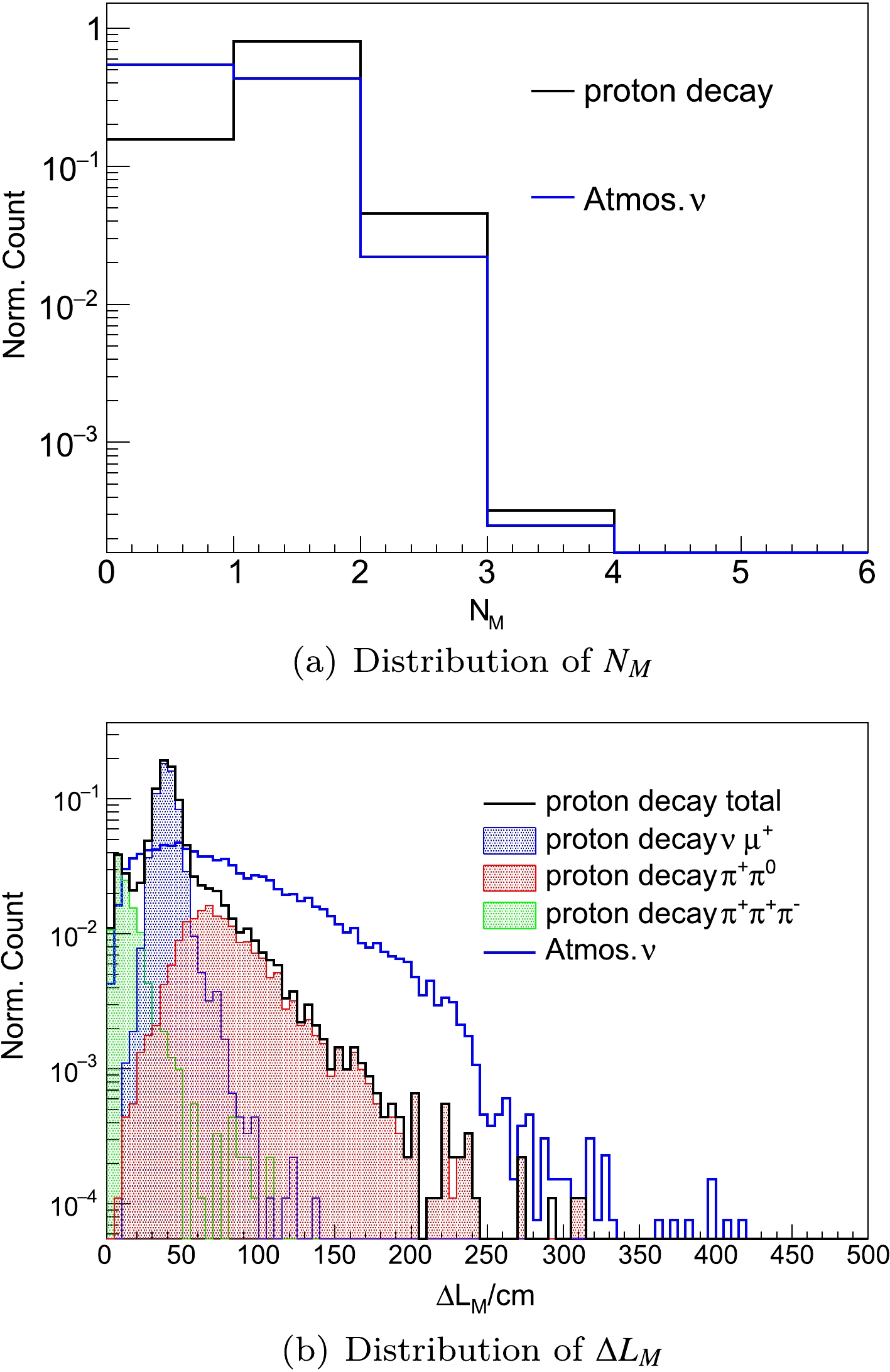
Figure 6. (color online)
$ N_M $ and$ \Delta L_{M} $ distributions of identified Michel electrons for$ p\to \bar{\nu} K^+ $ and atmospheric ν events with the basic selection and the selection of the time and energy properties of Michel electrons. Unit area normalization is used.(Cut-3): tagged Michel electron number
$ 1 \leq N_M \leq 2 $ ,(Cut-4): correlated distance
$ \Delta L_{M} \leq 80 $ cmin the remaining proton decay candidates after the basic selection. It can be found that 71.4% of
$ p\to \bar{\nu} K^+ $ and 9.2% of atmospheric ν events survive in the simulated event samples.Similar to the Michel electron, neutron capture is another potential selection criterion. Here, we assume that the delayed neutron capture signal can be fully identified by requiring the visible energy to lie within
$ 1.9 \,{\rm{MeV}} \leq E_n \leq 2.5 $ MeV and the correlated time difference to be 1$ \,{\rm{\mu s}} \leq \Delta T_{n} \leq 2.5 $ ms. In this way, 89.5% of the neutrons produced by atmospheric ν events can be distinguished. Fig. 7 shows the identified neutron distributions of$ p\to \bar{\nu} K^+ $ signals and backgrounds after the basic selections. The proton decay events have a smaller$ N_n $ on average than the atmospheric ν events. Therefore, we use the selection cut$ N_n \leq 3 $ to suppress the background. As shown in Fig. 7, the distance$ \Delta L_{n} $ , which is defined similar to$ \Delta L_{M} $ , can also be a powerful tool to reduce the backgrounds. Thus, a cut of$ \Delta L_{n} \leq 70 $ cm is required. Note that the criteria on$ N_n $ and$ \Delta L_{n} $ can reduce an important class of backgrounds, namely, events with a high energy neutron in the final state of the primary atmospheric ν interaction. Such a high energy neutron has a small probability of not losing its energy within 10 ns until it interacts with the LS to give a second pulse. If the final states include$ \mu^\pm $ or$ \pi^+ $ , this background event will mimic the three fold coincidence of$ p\to \bar{\nu} K^+ $ . Because a high energy neutron usually produces more neutrons and larger$ \Delta L_{n} $ , we choose the cuts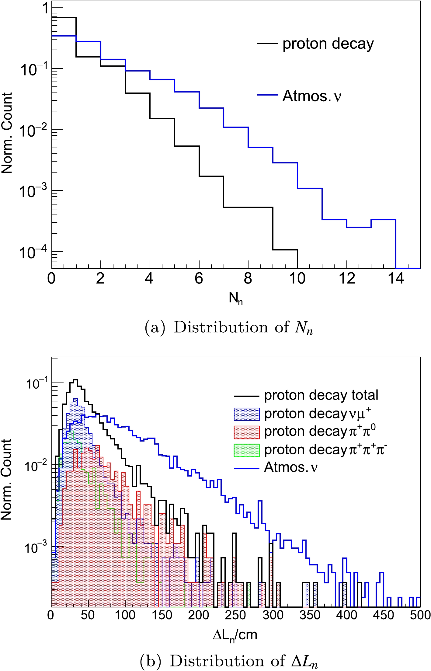
Figure 7. (color online)
$ N_n $ and$ \Delta L_{n} $ distributions of identified neutron capture for$ p\to \bar{\nu} K^+ $ and atmospheric ν events with the basic selection. Unit area normalization is used.(Cut-5): tagged neutron number
$ N_n \leq 3 $ for$ N_M=1 $ ,(Cut-6):
$ \Delta L_{n} \leq 70 $ cm if$ N_M=1 $ and$ 1 \leq N_n \leq 3 $ ,to suppress this type of background.
Based on the above discussions on delayed signals, we naturally classify the MC events into the following three samples:
Sample 1:
$ N_M=1,\Delta L_{M} \leq 80\;{\rm{cm}}, N_n = 0 $ ;Sample 2:
$N_M=1,\;\;\Delta L_{M} \leq 80\;\;{\rm{cm}},\;\;~ 1 \leq N_n \leq 3,\;\;\Delta L_{n} \leq$ $70 \; {\rm{cm}}$ ;Sample 3:
$ N_M=2, \Delta L_{M} \leq 80\;{\rm{cm}} $ .The survival rate of
$ p\to \bar{\nu} K^+ $ and the atmospheric ν events in the simulation can be found in Table 2. Approximately 6.8% of the total atmospheric ν events would survive, requiring further selection methods to reduce the background. -
As introduced in Sec. III.A, a
$ p\to \bar{\nu} K^+ $ event usually has a triple coincidence signature on its hit time spectrum. The first two pulses of the triple coincidence overlap each other in terms of the decay time of$ K^+ $ , which is a distinctive feature of$ p\to \bar{\nu} K^+ $ compared to the atmospheric ν backgrounds. This means that$ p\to \bar{\nu} K^+ $ can be distinguished from the backgrounds according to the characteristics of the overlapping double pulses. Therefore, the hit time spectrum is studied further using the multi-pulse fitting method [14] to reconstruct the time difference and energy of$ K^+ $ and its decay daughters.For each event, its hit time spectrum can be fitted with double-pulse
$ \phi_{D}(t) $ and single-pulse$ \phi_{S}(t) $ templates of the hit time t,$ \begin{eqnarray} \phi_{D}(t;\epsilon_{K}, \epsilon_{i}, a, \Delta T) = \epsilon_{K} \phi_{K}(t) + \epsilon_{i} \phi_{i}[a(t-\Delta T)], \end{eqnarray} $

(1) $ \begin{eqnarray} \phi_{S}(t;\epsilon_{S})= \epsilon_{S} \phi_{ \rm{AN}}(at), \end{eqnarray} $

(2) where
$ \phi_{K}(t) $ is the TOF-corrected template of$ K^+ $ ,$ \phi_{i}(t) $ is that of a decay daughter of$ K^+ $ , and$ i = \mu $ and π refer to the two dominant decay channels$ K^+ \to \mu^+ \nu_\mu $ for$ E_{\rm{vis}}\leq 400\;{\rm{MeV}} $ and$ K^+ \to \pi^+ \pi^0 $ otherwise, respectively. These templates are produced by the MC simulations in which the particles are processed by SNiPER with their corresponding kinetic energies.$\phi_{\rm{AN}}(t)$ is the template of the backgrounds, generated as the average spectrum of all the atmospheric ν events with energy depositions from 200 to 600 MeV. Owing to the influence of reflection, the hit time spectrum is widened when the energy deposition center is close to the boundary. To deal with this effect, the templates are separately produced in the inner (< 15 m) and outer volumes ($ > $ 15 m) and applied to the fitting of events in the corresponding volumes.In Eqs. (1) and (2),
$ \Delta T $ is the correlated time difference of the delayed component, a is a scaling factor to account for shape deformation of the second pulse caused by the electromagnetic showers, and$ \epsilon _{K} $ ,$ \epsilon _{i} $ , and$ \epsilon_{S} $ are the corresponding energy factors. They are free parameters in the fitting. For illustration, we use Eq. (1) to fit two typical events, as shown in Fig. 8.
Figure 8. (color online) Illustration of multi-pulse fitting to the hit time spectra of a proton decay event (left) and an atmospheric ν event (right). The x axis is the hit time after TOF correction. The black dots indicate the observed spectrum from the simulation. The blue line is the fitting result. The green and red filled histograms are the fitted result of the two components in the hit time spectrum, contributed by the
$ K^+ $ and$ K^+ $ decay daughters.After fitting the hit time spectra with the templates of Eqs. (1) and (2), we calculate
$ \chi^2 $ of the double and single pulse fittings using$ \chi_D^2= \sum \frac{[\phi(t)-\phi_D(t)]^2}{\sigma^2 [\phi(t)]} , $

(3) $ \chi_S^2= \sum \frac{[\phi(t)-\phi_S(t)]^2}{\sigma^2 [\phi(t)]}, $

(4) where
$\sigma^2 [\phi(t)] $ is the sample variance of the observed spectrum$\phi(t) $ at the t-th bin. The$ \chi ^2 $ ratio$ R_{\chi} \equiv \chi_S^2/\chi_D^2 $ is taken as a further selection criterion. From the double-pulse fitting using Eq. (1), the energies$ E_{1} $ and$ E_{2} $ of the overlapping double pulses from the depositions of the postulated$ K^+ $ and its decay daughters are calculated from$\epsilon_K $ ,$\epsilon_i $ , and a introduced in Eq. (1),$ E_{1}=\frac{\epsilon_K T_{K}}{\epsilon_K T_{K} + \epsilon_i T_{i}/a} E_{ \rm{fit}} $

(5) $ E_{2}=\frac{\epsilon_i T_{i}/a}{\epsilon_K T_{K} + \epsilon_i T_{i}/a} E_{ \rm{fit}}, $

(6) where
$ T_K = 105 $ MeV is the initial kinetic energy of$ K^+ $ from the free proton decay.$ T_\mu = 152 $ MeV and$T_\pi = 354 \;\rm{MeV}$ are the initial kinetic energies of the muon and pion from the$ K^{+} $ decay at rest. The fitted total energy is defined as$E_{\rm{fit}} = E_{\rm{vis}} - \sum E_M - \sum E_n$ , which is the visible energy minus the energies of Michel electrons and neutron capture.The way to select
$ p\to \bar{\nu} K^+ $ from the atmospheric ν backgrounds according to the parameters acquired above is introduced next. In Fig. 9, we plot the$ R_{\chi} $ distributions for proton decay and the atmospheric ν events after applying the selections from Cut-1 to Cut-6. We find that$ R_{\chi} $ is a tool to reject the background. In fact,$ R_{\chi} $ can be regarded as an indicator that the fitted event tends to be a double pulse overlapping event or a single pulse event. The larger the$ R_{\chi} $ , the stronger it tends to be an event with two pulses overlapping in the hit time spectrum. A cut of$ R_{\chi} >1 $ can be applied to roughly perform the selection. If$ R_{\chi} >1 $ , this fitted event may be preliminarily identified as a proton decay candidate. Otherwise, it would be rejected as a background candidate. However, a general cut of$ R_{\chi} $ is not justified to the three samples defined at the end of Sec. IV.B. Compared to Sample 1, which is composed of the common$ p\to \bar{\nu} K^+ $ and atmospheric ν events, Sample 2 is additionally composed of background events with energetic neutrons, as introduced in Sec. III.B. The second pulse caused by an energetic neutron gives these atmospheric ν events a fake double pulse overlapping shape in the hit time spectrum. A stricter requirement on$ R_{\chi} $ is consequently necessary to reduce the background.$ K^+ $ produced in the$ p\to \bar{\nu} K^+ $ events in Sample 3 decays via$ K^{+}\to\pi^{+}\pi^{+}\pi^{-} $ owing to the cut on the number of Michel electrons$ N_{M}=2 $ . As a result,$ p\to \bar{\nu} K^+ $ should be easier to distinguish from the backgrounds with$ N_{M}=2 $ . Therefore it is reasonable to set a less stringent cut on$ R_{\chi} $ to maintain a high detection efficiency. Consequently,$ R_{\chi} $ will be set separately for the three samples. To sufficiently reject atmospheric ν backgrounds, we require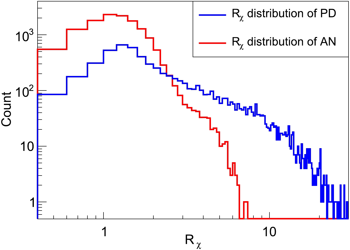
Figure 9. (color online) Distributions of the
$ \chi ^2 $ ratio$R_{\chi} \equiv $ $ \chi_S^2/\chi_D^2$ from$ p\to \bar{\nu} K^+ $ (PD) and atmospheric ν (AN) events after the basic and delayed signal selections.(Cut-7-1):
$ R_\chi > 1.1 $ for Sample 1,(Cut-7-2):
$ R_\chi > 2.0 $ for Sample 2,(Cut-7-3):
$ R_\chi > 1.0 $ for Sample 3.The distributions of fitted
$ \Delta T $ are shown in Fig. 10(a), where a rough cut of$ R_{\chi}>1 $ is applied to$ p\to \bar{\nu} K^+ $ and the backgrounds. From the figure, we find that$ \Delta T $ for the remaining backgrounds, which are mis-identified as$ p\to \bar{\nu} K^+ $ candidates, are mostly distributed at small$ \Delta T $ because atmospheric ν events are usually a single pulse. Meanwhile, when$ K^+ $ decays in a few nanoseconds, the fitting has low efficiency because both components are too close to be distinguished from each other (as shown in Fig. 10(b)). Consequently,$ \Delta T $ is required as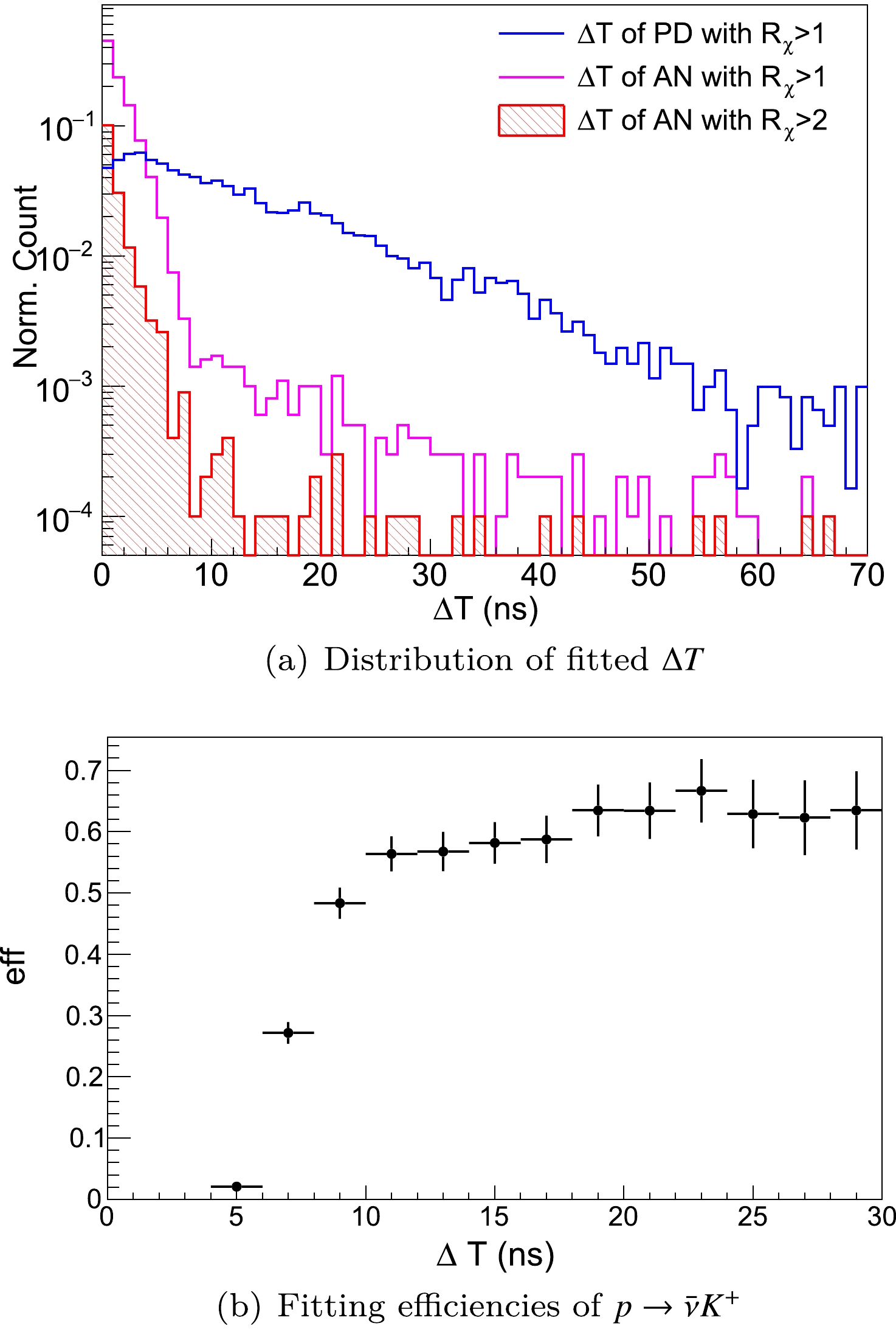
Figure 10. (color online)
$ \Delta T $ distribution and fitting efficiencies. (a) Distribution of fitted$ \Delta T $ (Eq. (1)) of$ p\to \bar{\nu} K^+ $ (PD, in blue) and atmospheric ν (AN, red filled and pink) events with different$ R_{\chi} $ cuts after the basic and delayed signal selections. (b) Fitting efficiencies for$ p\to \bar{\nu} K^+ $ with different true$ \Delta T $ ($ K^+ $ decay time). The efficiencies are low when$ K^+ $ decays within several ns because both pulse components are too close.(Cut-8): correlated time difference should be
$ \Delta T \geq 7 $ ns.Regarding the kinematics of
$ K^+ $ and its decay daughters, the sub-energy$ E_1 $ should be distributed from 0 to more than 200 MeV, with an average of 105 MeV, whereas$ E_2 $ should be fixed around 152 MeV or 354 MeV depending on the decay mode. As shown in Fig. 11, we plot the correlated sub-energy deposition distributions of$ p\to \bar{\nu} K^+ $ and the background events. Two obvious groups can be observed in the left panel, corresponding to the two dominant decay channels of$ K^+ $ . Only a small group of atmospheric ν events remains in the bottom right corner of the right panel of Fig. 11, which originates from the mis-identification of a tiny second peak. It is clear that a box selection on$ E_1 $ and$ E_2 $ can efficiently reject the atmospheric ν backgrounds. Therefore, the selections
Figure 11. (color online) Correlated
$ E_1 $ and$ E_2 $ distributions (in colored scale) for$ p\to \bar{\nu} K^+ $ (a) and atmospheric ν (b) events with the basic selection, delayed signal selection,$ R_{\chi} $ cut, and$ \Delta T $ cut. The events outside the red boxes are rejected as background. More details can be found in the text.(Cut-9-1):
$ 30 \, {\rm{MeV}} \leq E_1 \leq 200 $ MeV,(Cut-9-2):
$ 100 \, {\rm{MeV}} \leq E_2 \leq 410 $ MeV,are required. The lower boundary of
$ E_1 $ is set to avoid the influence of the coincidence with low energy events, such as reactor antineutrinos or radioactive backgrounds.The detection efficiencies under each selection criterion are listed in Table 2, where the number of remaining backgrounds are also shown, from which the elimination power of each criterion can be found. After applying these criteria, the total efficiency for
$ p\to \bar{\nu} K^+ $ is estimated to be 36.9%, and only one event in Sample 1 remains from the simulated 160 k atmospheric ν events (corresponding to an exposure of 890 kton-years or an exposure time of 44.5 years at the JUNO site). Because the volume cut in the basic selections provides a selection efficiency of 96.6% to the total efficiency, it will not be counted in the exposure mass calculation. The three samples contribute 27.4%, 7.3%, and 2.2% of the detection efficiencies, respectively. Considering the statistical error and weighting value, which accounts for the oscillation probability, the background level corresponds to 0.2 events, which is scaled to 10 years of data collection by JUNO. -
The detection efficiency uncertainties of
$ p\to \bar{\nu} K^+ $ are estimated and shown in Table 3. The statistical uncertainty is estimated to be 1.6% in the MC simulation. So far, we have been using the ideal setting for position reconstruction (30 cm for the energy deposition center position uncertainty without bias). Considering the performance of the vertex reconstruction algorithm, it is assumed that the residual bias of the position reconstruction of$ p\to \bar{\nu} K^+ $ is 10 cm. In this case, the efficiency uncertainty caused by a volume cut of 17.5 m is 1.7%.Source Uncertainty (%) Statistic 1.6 Position reconstruction 1.7 Nuclear model 6.8 Energy deposition model 11.1 Total 13.2 Table 3. Detection efficiency uncertainties for
$ p\to \bar{\nu} K^+ $ .Another important systematic uncertainty on the detection efficiency arises from the inaccuracy of the nuclear model, which influences the ratio of the accompanying particles of
$ p\to \bar{\nu} K^+ $ . To estimate this uncertainty, another$ p\to \bar{\nu} K^+ $ sample base is simulated with the FSI and de-excitation processes of the residual nucleus disabled. After applying all criteria, the difference in the detection efficiency is found to be 6.8%, which is the estimated uncertainty from the nuclear model.The dominant uncertainty originates from the energy deposition model. Owing to the lack of studies on sub-GeV particle behavior, especially the quenching effect of hundreds of MeV
$ K^+ $ in LAB based LS, the deposition simulation in the LS detector might be inaccurate. Therefore, the simulated waveform of the hit time spectrum may differ from the real one. According to the study of KamLAND [14], this type of uncertainty is estimated as 11.1%. We conservatively use this value considering the similar detection method. Therefore, the uncertainty of the proton lifetime is estimated as 13.2%, considering all the sources introduced above.The uncertainties of the background level in ten years is composed of two parts. The first is the systematic uncertainty contributed by the uncertainty of the atmospheric neutrino flux (20%) and atmospheric neutrino interaction cross-section (10%) [5]. Another uncertainty originates from the number
$ N_n $ of neutron capture, which can be affected by the secondary interactions of the hadronic daughter particles of atmospheric neutrino events in the LS. This is estimated as 10% assuming the same uncertainty as Super-K [30]. The statistic uncertainty is estimated following the$ 1/\sqrt{N} $ rule. Considering that only one event survives in the selection, it is calculated as$ \pm 0.2 $ in ten years. With 160 k events in the current MC simulation, this is difficult to improve because it will consume vast computing resources. We hope to update this value with a larger MC simulation data volume when it permits. Consequently, the background is estimated as$0.2\;\pm 0.05({\rm{syst}})\;\pm \; 0.2({\rm{stat}})$ .The sensitivity for
$ p\to \bar{\nu} K^+ $ is expressed as$ \begin{eqnarray} \tau / B(p \to \bar{\nu} K^+) = \frac{N_p T \epsilon}{n_{90}}, \end{eqnarray} $

(7) where
$ N_p = 6.75 \times 10^{33} $ is the total number of protons (including$ 1.45\times 10^{33} $ free protons and$ 5.3\times 10^{33} $ bound protons) in the JUNO CD, T is the running time, which is assumed to be 10 years to achieve an exposure mass of 200 kton-years,$\epsilon=36.9\% $ is the total signal efficiency, and$ n_{90} $ is the upper limit of the 90% confidence level of the detected signals. This depends on the number of observed events and the background level. According to the Feldman-Cousins method [31],$ n_{90} $ is estimated as 2.61 given an expected background of 0.2 in 10 years. Thus, the JUNO sensitivity for$ p\to \bar{\nu} K^+ $ at the 90% C.L. with 200 kton-years would be$ \begin{equation} \tau / B(p \to \bar{\nu} K^+) > 9.6 \times 10^{33} \, {\rm{years}}. \end{equation} $

(8) Compared to the representative LS detector, the detection efficiency on
$ p\to \bar{\nu} K^+ $ of JUNO is relatively lower than that of LENA [13]. This is reasonable considering that the study is based on an overall detector simulation of JUNO. Based on the background level of 0.02 events per year, we plot the JUNO sensitivity as a function of running time, as shown in Fig. 12. After six years of running (120 kton-years), JUNO will overtake the current best limit of the Super-K experiment.
Figure 12. (color online) JUNO sensitivity for
$ p\to \bar{\nu} K^+ $ as a function of running time.Moreover, the proton lifetime measured by JUNO will reach
$ 10^{34} $ years for the first time after 10.5 years of data collection. In the case of no event observation after ten years, the 90% C.L. limit on the proton lifetime would reach$ 1.1 \times 10^{34} $ years. In the case of one event observation (16.4% probability), the corresponding limit would be$ 6.0 \times 10^{33} $ years. -
A simulation study is conducted to estimate the performance of the JUNO detector in searching for proton decay via
$ p\to \bar{\nu} K^+ $ . It is found that the expected detection efficiency of$ p\to \bar{\nu} K^+ $ is 36.9% ± 4.9%, whereas the background is estimated to be$ 0.2\pm 0.05({\rm{syst}})\pm 0.2({\rm{stat}}) $ after ten years of exposure. Assuming no proton decay events are observed, the sensitivity of JUNO for$ p\to \bar{\nu} K^+ $ is estimated to be$ 9.6 \times 10^{33} $ years at the 90% C.L. based on a total exposure of 200 kton-years (or a live fiducial exposure of 193 kton-years). This is higher than the current best limit of$ 5.9\times10^{33} $ years from the excellent effort of the Super-K experiment with a live fiducial exposure of 260 kton-years [11].It shows that an LS detector such as JUNO will be competitive with the planned Hyper-Kamiokande [7] and DUNE [8] experiments. Using different target nuclei
$ ^{12} {\rm{C}} $ from the LS and the newly developed analysis method considering delayed signals (Michel electrons and neutron capture), JUNO will provide a complementary search to test the GUTs from the perspective of$ p\to \bar{\nu} K^+ $ . Besides the$ p\to \bar{\nu} K^+ $ mode, JUNO will have some sensitivity to the other nucleon decay modes listed in Ref. [4], particularly the decay modes that also exhibit the three fold coincidence feature in time, such as$ n\to \mu^- K^+ $ ,$ p\to e^+K^{*}(892)^{0} $ ,$ n\to \nu K^{*}(892)^0 $ , and$ p\to \nu K^{*}(892)^{+} $ . These will be analyzed in the future.
JUNO sensitivity on proton decay p → νK+ searches
- Received Date: 2023-01-10
- Available Online: 2023-11-15
Abstract: The Jiangmen Underground Neutrino Observatory (JUNO) is a large liquid scintillator detector designed to explore many topics in fundamental physics. In this study, the potential of searching for proton decay in the


 DownLoad: