


 Abstract
 HTML
HTML Reference
 Related
 PDF
PDF


-
Conventional studies on r-processes focus on producing heavy unstable nuclei. Among the thousands of publications, one may be impressed by the recent reviews [1–3].
The interesting aspects of the current study lie in the area of r-processes that occur with light 1p-shell nuclei and are motivated by the concepts suggested in Refs. [4–6]. Kajino et al. suggested networks for primordial nucleosynthesis in inhomogeneous Big Bang models in Ref. [4] and their further extension to the evolution of light elements in cosmic rays [5].
More than 20 years ago, Terasawa et al. raised the problem of the role of light neutron-rich nuclei (Z < 10) in r-process nucleosynthesis in supernovae [6]. In particular, we are interested in the possible branching of boron and carbon chains leading to the formation of heavier isotopes up to oxygen for the development of a primordial chain starting from 7Li (see Fig. 6 in Ref. [7] and our illustration in Fig. 1).
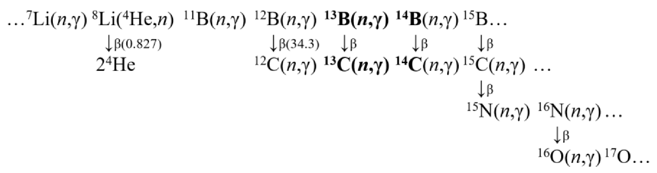
Further development of sensitivity studies on the (n, γ) reactions running through the neutron-rich boron 11–14B and 12–19C carbon isotopes was achieved by Sasaqui et al. [7], and these reactions have been included in heavy nuclei network production. Almost all reaction rates for the boron chains used in these model calculations were taken from [8], and their uncertainties were estimated to be at least a factor of two [7]. It turned out that only the 13B(n, γ)14B process on boron isotopes exhibited zero impact on heavy element production.
We suggest a new estimation of the 13B(n, γ)14B reaction rate within the modified potential cluster model (MPCM) approach, which significantly differs from the results of Ref. [8]. Therefore, we can provide reasons for revising the conclusions of [7] on the negligible role of the 13B(n, γ)14B reaction in heavy nuclei network production.
A comparative analysis of the reaction rates of the processes in Fig. 1 is a way of defining the contribution of the 13B(n, γ)14B reaction in the boron-carbon-nitrogen network. Our early MPCM research on neutron radiative capture reactions relevant to those in Fig. 1 is provided in the following references: the 10B(n, γ)11B reaction is examined in Ref. [9], the reaction chain 11B(n, γ)12B(n, γ)13B is considered in Refs. [10, 11, 12], we investigated 12C(n, γ)13С in Ref. [13] and 13С(n, γ)14С in Ref. [14], 14С(n, γ)15С is not yet published, and research on the 15N(n, γ)16N process is presented in Ref. [15].
For the reaction 16O(n, γ)17O, the measured cross-section and its rate, calculated in the direct reaction capture model, are presented in the recent Ref. [16]. There are no data on the 14B(n, γ)15B and 16N(n, γ)17N reaction rates to date.
Experimental study of the 13B(n, γ)14B reaction is presented using the only measurement of the neutron breakup of the 15B isotope via Coulomb dissociation performed in inverse kinematics [17]. The total cross-section of 13B(n, γ)14B is derived from the Coulomb breakup of 15B and is very tentative. Therefore, theoretical model calculations are in high demand to fill the information gap on the 13B(n, γ)14B reaction in boron chains as in Fig. 1.
Another problem concerns the lack of well-defined information on the spectral structure of 14B required to apply the MPCM. We use current data on the 14B spectrum [18], as opposed to previous data from an earlier review [19], to classify the possible multipole structure of the corresponding cross-sections of present and future interest.
Interestingly, the reactions 13B(n, γ)14B and 13C(n, γ)14C are isobar-analogous, and the latter is examined in detail in Ref. [14]. Although 14B and 14C are not mirror nuclei, the Young diagrams reveal several common features of orbital symmetry. We exploit this fact while classifying the allowed and forbidden states (FS) in the discrete and continuum spectra of n + 13B channels.
Within the MPCM, the total cross-sections of 13B(n, γ)14B radiative capture onto the ground state (GS) and first excited state (ES) of 14B are calculated, as well as the reaction rates in the interval 0.01T9 – 10T9. Based on the reaction rate interval, we evaluate the balance between 14B synthesis via the radiative neutron capture reaction 13B(n, γ)14B and 13B decay inhibiting this synthesis.
This paper is organized as follows. Sec. II contains the MPCM presentation of 14B in the n + 13B channel. In Sec. III, the total cross-sections of the 13B(n, γ0+1)14B reaction are considered. In Sec. IV, we present the n13B radiative capture reaction rate and compare the neutron radiative capture rates on 10-13B and 12-14C isotopes. We outline the conclusions in Sec. V. Appendix A includes the numerical values of the n13B reaction rate, and Appendix B illustrates the computational procedure accuracy of the reaction rate calculations.
-
We preface the calculations of the reaction cross-sections with an analysis of the 14B spectrum data, following Ref. [18]. The spectrum of selected levels of the 14B nucleus is shown in Fig. 2. The structure of the bound ground state Jπ, T = 2–, 2 is assigned as a combination of two main orbital components:
${\psi _{GS}} = {\alpha _S}\left| S \right\rangle + {\alpha _D}\left| D \right\rangle + ...$ , where the corresponding weights are${\alpha _S} = 0.71(5)$ and${\alpha _D} = 0.17(5)$ . In the present calculations, we consider the S-component only. As for the excited Jπ = 1– state, it is found to be the dominant S-component with a weight${\alpha _S} = 0.94(20)$ .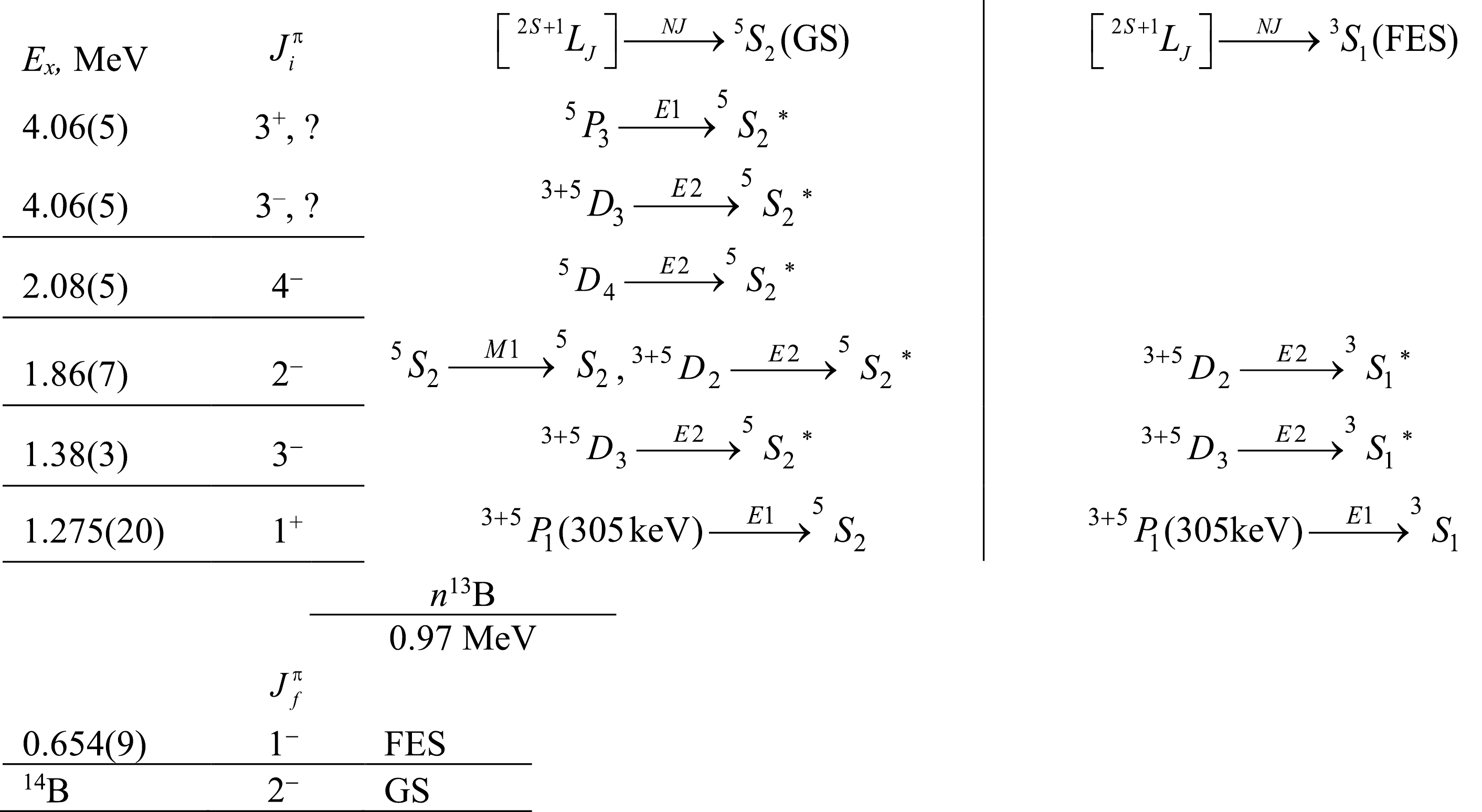
Figure 2. Spectrum of the 14B nucleus in MeV [18]. * indicates the transitions we do not consider.
Now, let us comment on the resonance states in the spectrum of 14B. The 1st resonance can be associated with the spin-mixed 3+5P1 wave at the energy Ec.m. = 0.305(20) MeV because Jπ = 3/2– for 13B and Jπ = 2– for 14B. Radiative neutron capture from this state proceeds via the E1 transition to the ground 5S2 and excited 3S1 states.
The 2nd resonance has Jπ = 3– and may be excited at 0.41 MeV as a 3+5D2 state so that only the E2 transition may occur. Because we are operating within the long-wave approximation for the electromagnetic interaction Hamiltonian here and henceforth, we do not consider the E2 or M2 transitions if selection rules do not forbid the more strong E1 and M1 processes.
The 3rd resonance with Jπ = 2– may be excited at 0.89(7) MeV in the 5S2 or 3+5D2 scattering waves. From the 5S2 scattering wave, the M1 transition to the GS is allowed, but we assume that owing to the large width Γc.m. =1.0(5) MeV, this resonance does not practically affect the total capture cross-section if this resonance is considered a spin-mixed 3+5D2 wave.
The 4th resonance at an excitation energy of 2.08(5) MeV is defined as the Jπ = 4– state, but its width is unknown. It may be matched to a 5D3 scattering wave, leading to the E2 transition, and is not considered in present calculations.
The position of the 5th resonance in the spectrum is defined at 4.06(5) MeV, with a width of 1.2(5) MeV and a total spin J = 3, but the parity is unknown [18]. We assume a positive parity for this level and construct a resonance potential for the 5P3 scattering wave. The 5P3 state leads to the E1 transition to the 5S2 ground state of 14B. Its effect on the total cross-section is weak owing to its large width. If a negative parity is assumed, this state is the analog of the 2nd resonance state mentioned above.
We do not denote two other levels in the spectrum at energies of 2.32(4) MeV and 2.97(4) MeV because only their energies are known [18]. Transitions labeled as not considered in Fig. 2 may be assumed as perspectives for future study of the 13B(n, γ)14B reaction when new experimental data on the 14B spectrum are available.
-
The cross-sections of E1 and M1 capture to the GS are provided by the following transition amplitudes:
$\begin{aligned}[b]& ^{3 + 5}{P_1}(305\;{\text{keV}}){\xrightarrow{{E1}}^5}{S_2}, \quad ^5{P_3}{\xrightarrow{{E1}}^5}{S_2}, \quad ^{3 + 5}{P_2}{\xrightarrow{{E1}}^5}{S_2},\\& ^3{P_0}{\xrightarrow{{E1}}^5}{S_2},\quad ^5{S_2}{\xrightarrow{{M1}}^5}{S_2}.\end{aligned} $

(1) For the cross-sections of E1 and M1 capture to the ES of 14B, these transition amplitudes are
$ ^3{P_1}(305\;{\text{keV}}){\xrightarrow{{E1}}^3}{S_1} , ^3{P_0}{\xrightarrow{{E1}}^3}{S_1} , ^3{P_2}{\xrightarrow{{E1}}^3}{S_1} , ^3{S_1}{\xrightarrow{{M1}}^3}{S_1} . $

(2) The calculation of the corresponding cross-sections is performed using the following formalism [20–23] adapted to the selected E1 and M1 transitions:
$ \sigma (N1,{J_f}) = \frac{{2\pi {{\rm e}^2}}}{{3{\hbar ^2}}}{\left( {\frac{{\mu K}}{{k }}} \right)^3}\sum\limits_{{L_i},{J_i}} {(2{J_i} + 1) \cdot {B^2}(N1) \cdot I_{NJ}^2(k,{J_f},{J_i})} , $

(3) $ {B^2}(E1) = \frac{{25}}{{m_{{}^{13}{\text{B}}}^2}}, {I_{EJ}}(k,{J_f},{J_i}) = \left\langle {{\chi _f}\left| {{r^J}} \right|{\chi _i}} \right\rangle ,$

(4) $\begin{aligned}[b]& {B^2}(M1) = 3{\left( {\frac{\hbar }{{{m_0}c}}} \right)^2}{\left[ {\frac{{{\mu _n}}}{{{m_n}}} - \frac{{{\mu _{{}^{13}{\text{B}}}}}}{{{m_{{}^{13}{\text{B}}}}}}} \right]^2}, \\&{I_{MJ}}(k,{J_f},{J_i}) = \left\langle {{\chi _f}\left| {{r^{J - 1}}} \right|{\chi _i}} \right\rangle, \end{aligned}$

(5) where N1 = E1 or M1, μ is the reduced mass in the n + 13B channel, K is the γ-quantum wave number,
$K = {E_\gamma }/\hbar c$ , k is the relative motion wave number related to the non-relativistic kinetic energy as${E_{\rm c.m.}} = {\hbar ^2}{k^2}/2\mu $ , Ji and Jf are the total angular momenta, the multipolarity is fixed as the dipole J = 1, and${I_{NJ}}(k,{J_f},{J_i})$ are the radial matrix elements over the relative distance r. We use masses of mn = 1.00866491597 amu [24] and$m_{{}^{13}{\text{B}}}^{}$ = 13.0177802 amu [25], and the constant$ {\hbar ^2}/{m_0} $ = 41.4686 MeV·fm2, where m0 is the atomic mass unit (amu). The magnetic moments in (5) are given in nuclear magneton μN: μn = −1.9130μN, and${\mu _{{}^{13}{\text{B}}}}$ = 3.1778 μN [18, 19, 24, 25].The radial functions χi and χf are the numerical solutions of the Schrodinger equation, with the central interaction potential of Gaussian type for a fixed combination of angular momenta JLS,
$ V\left({}^{2S+1}{L}_{J},r\right) = -{V}_{0}\left({}^{2S+1}{L}_{J}\right)\text{exp}\left\{-\alpha \left({}^{2S+1}{L}_{J}\right){r}^{2}\right\}, $

(6) where the potential parameters V0 and α depend on the momenta [2S+1LJ]i, f of the partial wave.
Following (1) and (2), the S and P waves provide the transition amplitudes in the initial continuum channel. The classification of orbital states using Young diagrams for the 14-nucleon system in the channel A = 13 + 1 proves that only S waves are allowed, and P waves also have a forbidden state [14]. Because there are no complete tables of the products of Young diagrams for a system with A > 8, we complement the symmetry analysis with the formalism of the translationally invariant shell model (TISM) [26, 27]. Therefore, we treat the option of the interaction potential with FS for S waves.
The classification of orbital states using Young diagrams defines the optimization range of the potential depth V0, i.e., if FS exists in the given channel, the potential should be sufficiently deep to include this state. Otherwise, it may be shallow. Shallow potentials are appropriate for the description of scattering states without resonances and should give phase shifts close to zero [22, 23]. Deep non-resonance potentials should also provide the moderate energy dependence of phase shifts, which may be normalized according to the Levinson theorem (see details in [28]). In the case of resonance scattering states, the potential (6) should fit additional conditions – the reproduction of the resonance position Ec.m. and its width Γc.m. within the experimental uncertainties [11, 20].
We provide the potential parameters of the neutron scattering on 13B in Table 1.
No. {2S+1LJ}i V0/ MeV α/ fm−2 1 3+ 5P1 – resonance at 305 keV 618.035 0.8 2 3+5P2, 5P3, 3P0 – non-resonance 1220.0 1.0 3 5S2, 3S1 – non-resonance 0.0 0.0 4 5S2 – non-resonance 315.0 1.0 Table 1. Parameters of the interaction potentials of the n + 13B continuum.
Parameters of the 3+5P1 wave potential are matched with the experimental values of the resonance position Ec.m. = 305(20) keV and width Γc.m. = 100(20) keV [18]. Calculations with potential No. 1 in Table 1 lead to Ec.m. = 305(1) keV and Γc.m. = 106(1) keV. The corresponding 3+5P1 phase shift shown in Fig. 3 (red solid curve) reveals the resonant behavior and equals 270(1)° at 305 keV.
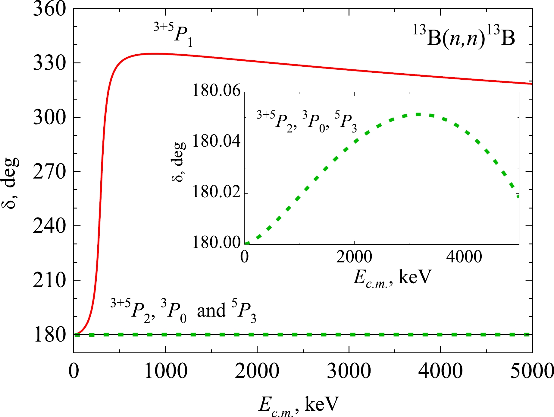
Figure 3. (color online) P wave phase shifts calculated in the MPCM with the parameters in Table 1: red solid curve – resonance 3+5P1 wave, green dashed curve – non-resonance 3+5P2, 3P0, and 5P3 waves.
Non-resonance 3+5P2, 5P3, and 3P0 waves are provided by potential No. 2 with FS from Table 1. Their phase shifts are normalized to 180(1)° according to the generalized Levinson theorem [28] (green dashed curve in Fig. 3).
For the non-resonance S-waves, we consider two variants of the interaction potentials. No. 3 from Table 1 refers to the case without FS and leads to a zero scattering S-phase shift. The inclusion of FS leads to a 180(1)° phase shift with the No. 4 parameters from Table 1. The construction of BS potentials is based on the demand to reproduce the channel binding energy Eb and match the corresponding asymptotic constant.
We use the well-known relation for the asymptotic normalizing coefficient ANC and dimensionless asymptotic constant CW [22, 23],
$ {C_W} = \,\frac{{{A_{\rm NC}}}}{{\sqrt {2{k_0}} }} \cdot \frac{1}{{\sqrt {{S_{{f}}}} }} , $

(7) where the relative wave number k0 is related to the binding energy
$ {E_b} = {\hbar ^2}k_0^2/2\mu $ , and Sf is the spectroscopic factor. Note that experimental data on ANC usually found from the peripherical reactions alone with the spectroscopic factor Sf are the input information for calculations of the theoretical values CW. Ref. [29] reported the values ANC = 0.73(10) fm−1/2, obtained from measurements of the breakup cross-sections for the reaction 9Be(14B, 13B+γ)X at the National Superconducting Cyclotron Laboratory (NSCL), Michigan State University. Data on the spectroscopic factors Sf = 0.71(19) [30] and Sf = 0.66 [31] lead to the interval 0.52 ≤ Sf ≤ 0.9. Consequently, the range for the dimensionless constant is CW = 1.40(38).There are a number of phase shift equivalent potentials, which reproduce the channel binding energy exactly but lead to different radial wave functions. We exploit the CW constant to constrain the choice of the corresponding potential parameters. The asymptotic constant CW is not single-defined but has a range arising from experimental ANC and Sf values. There is also a variety of V0 and α parameters, which provide the binding energy Eb in the n + 13B channel within the CW range. This is shown in the band for the corresponding cross-sections. For example, the details of the computing methods we use may be found in Ref. [20].
The parameters of the GS potentials of 14B in the n13B channel given in Table 2 reproduce a binding energy of Eb = −0.9700 MeV. The potentials of the GS Nos. 1, 2 and 3, 4 have nearly the same CW in pairs and allow us to present the effects of the FS.
No. {2S+1LJ}i V0/ MeV α/ fm−2 CW Rch/ fm Rm/ fm 1 5S2 without FS 19.0756 0.2 1.40(1) 2.50 2.62 2 5S2 with FS 217.486 0.5 1.42(1) 2.50 2.63 3 5S2 without FS 6.1237 0.04 2.10(1) 2.52 2.81 4 5S2 with FS 49.262 0.1 2.15(1) 2.52 2.84 Table 2. Parameters of the GS potentials of 14B in the n13B channel and calculated asymptotic constant CW, Rch, and Rm radii.
The charge Rch and matter Rm radii are calculated with these parameter sets according to the procedure in Ref. [32]. To calculate the 14B radii, we use the following input information: for 13B, the known values are Rch(13B) = 2.48(3) fm and Rm(13B) = 2.41(5) fm [33]; the neutron matter radius is equal to the proton one, Rm(n) = Rm(p) = 0.8414(19) fm [24], and the neutron charge radius Rch(n) = 0. The obtained results for 14B listed in Table 2 are in good agreement with the experimental values Rch(14B) = 2.50(2) fm and Rm(14B) = 2.52(9) fm of Ref. [33].
The ES potentials of 14B in the n13B channel with the parameters given in Table 3 reproduce the binding energy Eb = 0.3160 MeV [32]. There is no data on ANC of the excited 1- state; therefore, the corresponding CW constants in Table 3 as well as the Rch and Rm radii may be recommended for future measurements. Along with Table 2, the potentials of the ES Nos. 1, 2 and 3, 4 are grouped in pairs for the same purpose to monitor the FS effects.
No. {2S+1LJ}i V0/MeV α/ fm−2 Cw Rch/fm Rm/fm 1 3S1 without FS 15.75681 0.2 1.21(1) 2.53 2.97 2 3S1 with FS 208.3937 0.5 1.22(1) 2.53 2.98 3 3S1 without FS 4.27985 0.04 1.53(1) 2.56 3.23 4 3S1 with FS 44.71865 0.1 1.56(1) 2.56 3.27 Table 3. Parameters of the ES potentials of 14B in the n13B channel and calculated asymptotic constant CW, Rch, and Rm radii.
Note that the interaction potentials may depend on different diagrams for the same orbital L-waves of continuous and discrete spectra [34]. The S-wave potentials in Table 1 for the continuum and Tables 2 and 3 for the bound states are different. This is an important observation in the case of M1 transitions. Otherwise, the radial matrix elements in (5) at J = 1 are equal to zero owing to the orthogonality of the bound and scattering radial functions calculated in the same potential.
-
The effect of the asymptotic CW constant on the total cross-sections for 13B(n, γ0)14B capture to the GS of 14B is illustrated in Fig. 4 (a). The results of the calculations of the E1 and M1 partial cross-sections for potentials Nos. 1 (CW = 1.40) and 3 (CW = 2.10) from Table 2 and the scattering potentials from Table 1 are shown in comparison with the experimental data of [17]. Figure 4 (a) shows the total cross-sections in the linear energy scale up to 2.5 MeV to display the
$ ^{3 + 5}{P_1} $ resonance at 305 keV.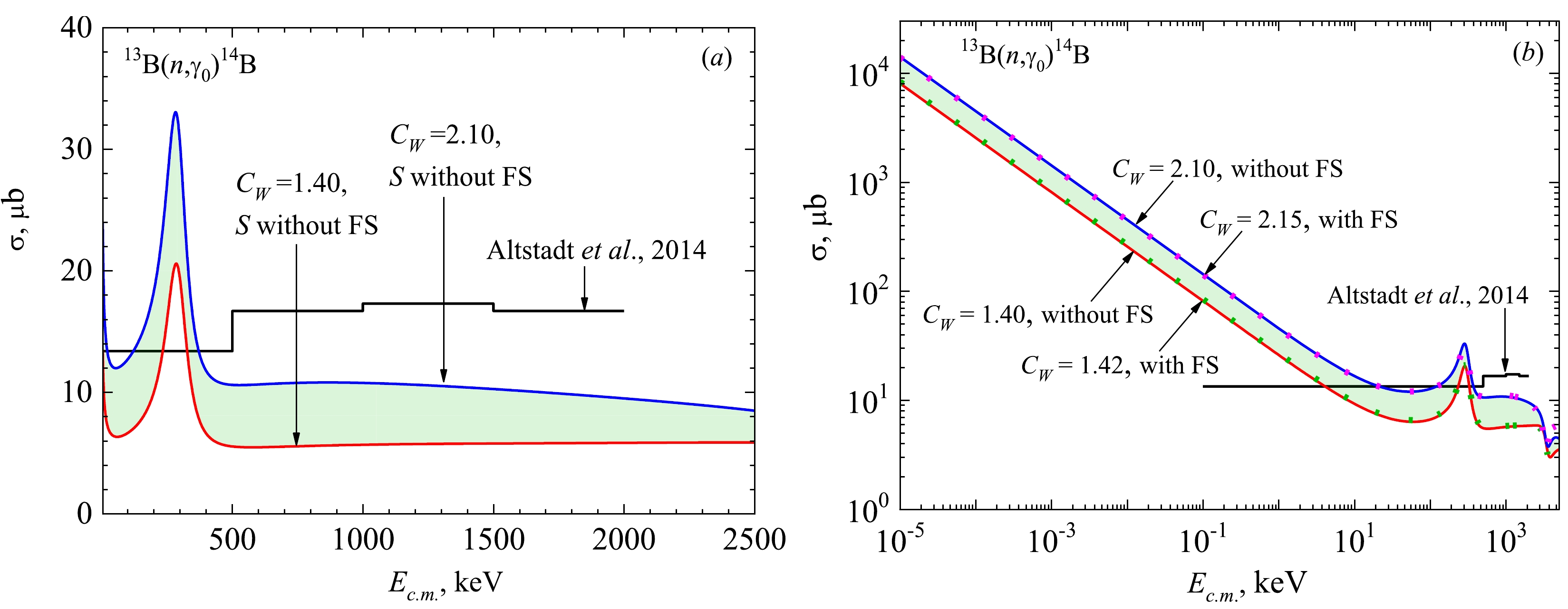
Figure 4. (color online) Total cross-sections of 13B(n, γ0)14B radiative capture to the GS of 14B with potentials from Tables 1 and 2. The histogram represents the experiment [17]. (a) Total cross-sections calculated without FS: red solid curve – potential No. 1 in Table 2 (CW = 1.40), blue solid curve – potential No. 3 in Table 2 (CW = 2.10). (b) Comparison of the total cross-sections calculated without and with FS: solid curves are the same as in Fig. 4 (a), green dotted curve – potential No. 2 in Table 2 (CW = 1.42), magenta dotted curve – potential No. 4 in Table 2 (CW = 2.15).
Figure 4 (b) shows a wider range from 10-5 keV to 5 MeV relevant to the reaction rate calculation (see Sec. IV). The purpose of the results presented in Fig. 4 (b) is to answer the question of the role of the FS in the GS potentials from Table 2 arranged in pairs, i.e., with or without FS at close CW. The calculation results of the total cross-sections for the GS potentials with FS Nos. 2 (CW = 1.42) and 4 (CW = 2.15) are shown in Fig. 4 (b) by the green and magenta dotted curves, respectively.
We find good pairwise agreement with the results for potentials without FS. The slight variation is associated with a small difference in the values of CW and the scattering phase shifts of the S potential with FS (No. 4 in Table 1) from exactly zero within 1 degree. At an energy of 10-5 keV, the cross-section value for the GS potential without FS No. 1 is equal to 8.05 mb, and for the GS with FS No. 2, it is equal to 8.36 mb. Similar results are obtained for the second potential with an FS. Therefore, we conclude that the presence or absence of FS does not affect the calculated total cross-section. The same consistent pattern is revealed in the (n, γ1) capture calculations to the ES of 14B. Further results are presented only for potentials without FS.
To evaluate the thermal cross-sections, we use the standard approximation at energies from 10 meV to 1 keV,
$ {\sigma _{\rm ap}}({\text{μb}}) = \frac{A}{{\sqrt {{E_{\rm c.m.}}({\text{keV}})} }}. $

(8) The value of the calculated cross-section
${\sigma _{\rm theor}}(E)$ at Emin = 10 meV provides the constant A = 25.46 μb·keV1/2 for the red solid curve in Fig. 4 (b) (CW =1.40). Consequently, at a thermal energy of 25.3 meV, the cross-section${\sigma _{\rm therm}}$ = 5.1 mb. For the blue solid curve in Fig. 4 (b) (CW = 2.10), A = 44.70 μb·keV1/2 and${\sigma _{\rm therm}}$ = 8.9 mb.The accuracy of the approximation (8) is defined by the relative difference between the cross-sections
${\sigma _{\rm theor}}(E)$ and σap (E),$ M(E) = \left| {[{\sigma _{\rm ap}}(E) - {\sigma _{\rm theor}}(E)]} \right|/{\sigma _{\rm theor}}(E). $

(9) M(1 keV) ≈ 0.2% for both cases of CW decreases with decreasing energy.
Figure 5 illustrates the input of the partial E1 and M1 cross-sections related to the set of amplitudes (1) of the (n, γ0) process. The M1 transition from the S wave determines the low-energy and thermal cross-sections. The E1 transition amplitudes define the higher energy region. The (n, γ1) capture process reveals nearly the same partial structure (2).
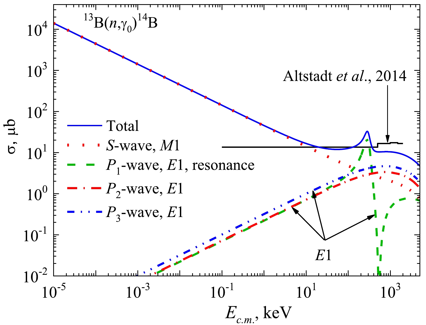
Figure 5. (color online) Partial E1 and M1 and total cross-sections of 13B(n, γ0)14B radiative capture to the GS of 14B (CW = 2.10 without FS). The histogram represents the experiment [17].
Figure 6 illustrates the relative input of the (n, γ0) and (n, γ1) capture processes into the total cross-section. The dominance of the (n, γ0) cross-section compared with (n, γ1) is within a factor of ~ 1/30. Note that the example in Fig. 6 refers to the lower CW values. The tendency is as follows: an increase in CW leads to the increase of any cross-section, but the (n, γ0) dominance remains within the above factor.

Figure 6. (color online) Partial E1 and M1 and total cross-sections of 13B(n, γ0+1)14B radiative capture to the ground 2– and excited 1– states of 14B (CW = 1.40 for the GS and CW = 1.21 for the ES). The histogram represents the experiment [17].
Summarizing our results for the total cross-sections in Figs. 4−6, we find that starting from Ec.m. ≈ 10 keV and down to thermal energies, the cross-section increases by 103 times from ~ 10 μb to ~ 5–10 mb. We assume this result is a prospective one for future experiments. At the same time, because the data of [17] are preliminary and not sufficiently informative, our discussions on the agreement between the experiment and MPCM calculations in Figs. 4, 5, and 6 are slightly premature.
-
We follow [35] when calculating the reaction rate of radiative neutron capture. For the rate in units of cm3mol-1sec-1, the following expression is used:
$\begin{aligned}[b] {N_A}\left\langle {\sigma v} \right\rangle =& 3.7313 \cdot {10^4}{\mu ^{ - 1/2}}T_9^{ - 3/2}\int\limits_0^\infty {\sigma (E)} E\\&\times\exp ( - 11.605E/{T_9}){\rm d}E, \end{aligned}$

(10) where NA is Avogadro's number, E is given in MeV, the total cross-section σ(E) is in μb, μ is the reduced mass in amu, and T9 is the temperature in 109 K [35]. Appendix B illustrates the computational procedure accuracy of the reaction rate calculations.
-
In Fig. 7 (a), the red and blue solid curves show the (n,γ0) capture reaction rates to the GS, which correspond to the results for the total cross-sections presented for the potentials without FS in Fig. 4 (b). The band in Fig. 7 (a) corresponds to the band in Fig. 4 and confines the possible reaction rate values for the range of CW discussed in Sec. II.B.
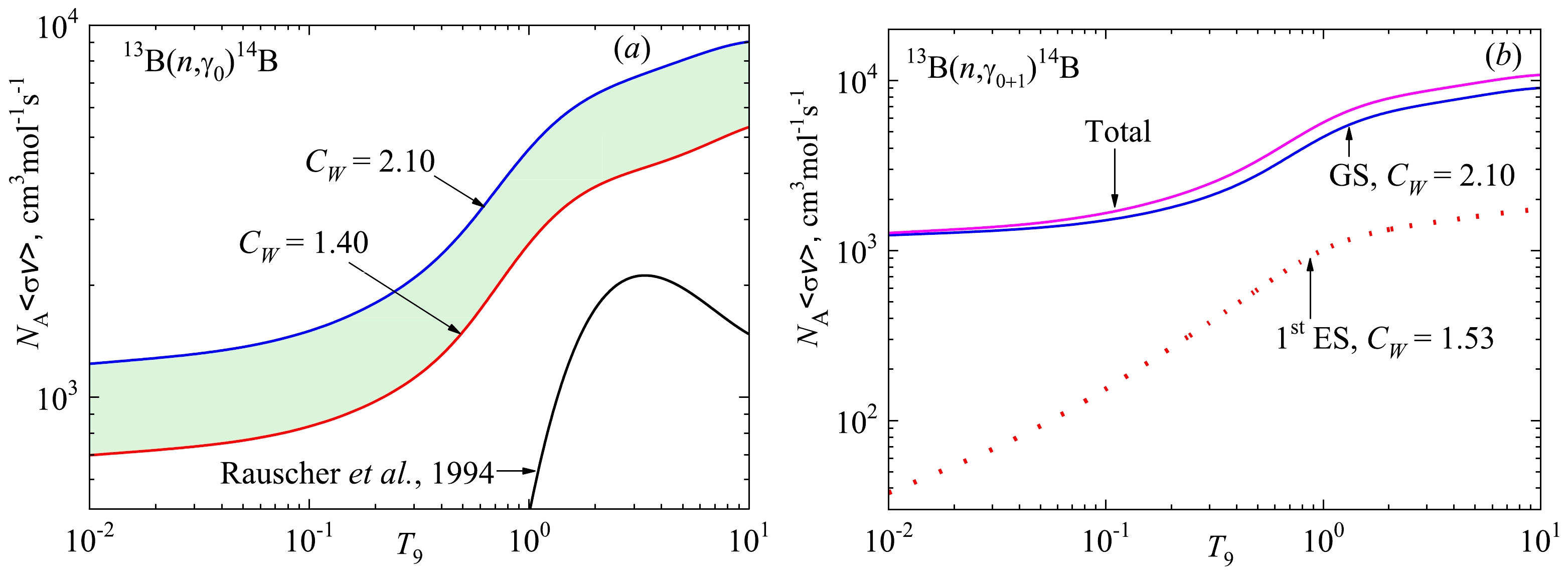
Figure 7. (color online) Reaction rate of radiative neutron capture on 13B calculated with potentials without FS. (a) Transitions to the GS: potential No. 1 from Table 2 (CW = 1.40) – red solid curve, potential No. 3 from Table 2 (CW = 2.10) – blue solid curve. The black solid curve shows the reaction rate obtained by Rauscher et al. in Ref. [8]. (b) Transitions to the ground and excited states: GS potential No. 3 from Table 2 (CW = 2.10) – blue solid curve; ES potential No. 3 from Table 3 (CW = 1.53) – red dotted curve. The magenta solid curve is the total capture reaction rate.
The black solid curve in Fig. 7 (a) shows the reaction rate from [8] obtained by Rauscher et al. Figure 7 (a) indicates that these results completely disregard the non-resonance part of the reaction, which leads to an increase in the cross-sections at low energies owing to the M1 transition, as shown in Fig. 4 (b) and Fig. 6.
An important remark concerns the structure of bound states. In [8], the D component is assumed for both the GS and ES of 14B in the n + 13B channel, in contrast with our treating these states as S-waves. Consequently, there are no M1 transitions in the calculations of Rauscher et al. [8], which provide the low-temperature reaction rate. The resonance structure of the black curve in Fig. 7 is due to the 3- (Ex = 1.38 MeV) resonance, and the 1+ resonance (Ex = 1.275 MeV) is not considered. The signature of the 1+ (305 keV) resonance in the cross-sections in Figs. 4–6 incorporated in the current calculations is observed in reaction rates as an increase at temperatures of T9 ≥ 0.2 in Fig. 7.
Figure 7 (b) shows the input of the (n, γ1) capture to the reaction rate through the example of one CW set. As shown in Fig. 6, the (n, γ1) capture contribution of the excited 1- state is relatively small, resulting in the values of the reaction rate in Fig. 7 (b) (red dotted curve). The same tendency is preserved for any other CW set.
The signature of the 300 keV resonance in the cross-sections in Figs. 4–6 is observed in the reaction rates as an increase at temperatures of T9 ≥ 0.2 in Fig. 7.
The reaction rates in Fig. 7 are parameterized by an expression of the form [36]
$ \begin{aligned}[b]{N_A}\left\langle {\sigma v} \right\rangle =& {a_1}/T_9^{2/3}\exp ( - {a_2}/T_9^{1/3})(1.0 + {a_3}T_9^{1/3} \\&+ {a_4}T_9^{2/3} + {a_5}T_9^{} + {a_6}T_9^{4/3} + {a_7}T_9^{5/3}) + \frac{{{a_8}}}{{{T_9}}}.\end{aligned} $

(11) The parameters ai given in Table 4 correspond to the reaction rates presented in Fig. 7: the first column refers to the red solid curve in Fig. 7 (a); the second column – the blue solid curve in Fig. 7 (a); the third column – the red dotted curve in Fig. 7 (b); the last column – the magenta solid curve in Fig. 7 (b).
i (n, γ0), CW = 1.40 (n, γ0), CW = 2.10 (n, γ1), CW = 1.53 (n, γ0+1), CW = 2.10 and CW = 1.53 ai ai ai ai 1 14381.77 17240.08 2413.837 19795.34 2 1.41717 1.2962 1.46568 1.31492 3 −2.61253 −2.52512 −3.81023 −2.64425 4 1.16178 0.93077 4.53362 1.25477 5 3.19007 3.74616 2.12766 3.6103 6 −2.58617 −2.76411 −2.80537 −2.77072 7 0.57029 0.57636 0.69249 0.58652 8 4.74344 7.39244 0.13587 7.62151 χ2 = 0.13 χ2 = 0.09 χ2 = 0.12 χ2 = 0.09 Table 4. Parameters in (11) for the reaction rates in Fig. 7.
The reaction rates are presented in Table A1 of Appendix A.
T9 (n, γ0), CW = 1.40 ${N_A}\left\langle {\sigma v} \right\rangle $ 

(n, γ0), CW = 2.10 ${N_A}\left\langle {\sigma v} \right\rangle $ 

(n, γ1), CW = 1.53 ${N_A}\left\langle {\sigma v} \right\rangle $ 

(n, γ0+1), CW = 2.10 and CW = 1.53 ${N_A}\left\langle {\sigma v} \right\rangle $ 

0.01 696.895 1227.53 37.5176 1265.0476 0.02 718.923 1270.56 53.8965 1324.4565 0.03 734.56 1302.34 67.2893 1369.6293 0.04 749.033 1332.05 80.0969 1412.1469 0.05 763.127 1361.07 92.6427 1453.7127 0.06 777.063 1389.77 105.014 1494.784 0.07 790.928 1418.33 117.244 1535.574 0.08 804.764 1446.79 129.351 1576.141 0.09 818.593 1475.22 141.346 1616.566 0.1 832.43 1503.63 153.236 1656.866 0.2 972.988 1789.64 267.522 2057.162 0.3 1123.68 2088.81 376.527 2465.337 0.4 1296.14 2417.88 483.691 2901.571 0.5 1496.05 2783.22 589.108 3372.328 0.6 1717.03 3173.33 690.019 3863.349 0.7 1946.46 3568.69 783.394 4352.084 0.8 2172.32 3951.72 867.368 4819.088 0.9 2386.04 4310.64 941.37 5252.01 1 2582.75 4639.3 1005.75 5645.05 1.5 3291.73 5830.41 1217.32 7047.73 2 3672.32 6500.93 1325.54 7826.47 2.5 3894.09 6920.42 1392.2 8312.62 3 4046.34 7223.52 1441.32 8664.84 3.5 4169.1 7469.1 1481.95 8951.05 4 4279.75 7682.51 1517.62 9200.13 4.5 4385.5 7874.58 1549.74 9424.32 5 4488.98 8049.78 1578.96 9628.74 6 4690.21 8355.32 1629.74 9985.06 7 4879.33 8603.13 1671.11 10274.24 8 5049.62 8794.33 1703.62 10497.95 9 5196.07 8931.47 1727.77 10659.24 10 5316.06 9018.76 1744.08 10762.84 χ2 = 0.13 χ2 = 0.09 χ2 = 0.12 χ2 = 0.09 Table A1. 13B(n, γ)14B radiative capture reaction rates.
-
To define the role of the 13B(n, γ )14B reaction in the boron chain of sequence in Fig. 1, we must consider whether the calculated reaction rates prove the formation of 14B or 13B decays before neutron capture may start. Short-lived isotopes may provide r-processes in an explosive environment and neutron-rich matter at high densities [37]. The conventional density–temperature conditions for the r-process are assumed as
$ {\bar n_n} $ ~ 1022 – 1023 cm−3 and T9 ~ 1 [2, 38]. We examine these conditions for the 13B(n, γ)14B reaction based on the calculated reaction rates.We can identify the r-process according to the following relation:
$ {\tau _\beta } \approx {N_n}\tau (n,\gamma ), $

(12) where the mean lifetime of β-decay τβ and neutron capture time
$ \tau (n,\gamma ) $ are interrelated by the number of neutrons Nn that must be captured before β-decay occurs [37, 39]. The neutron capture time$ \tau (n,\gamma ) $ depends on the reaction rate and neutron number density$ {\bar n_n} $ [40],$ \tau (n,\gamma ) = \frac{1}{{{{\bar n}_n}\left\langle {{\sigma _{n,\gamma }}v} \right\rangle }} . $

(13) Note that the recommended half-life values t1/2 [18, 41, 42] span the range 17.10 – 17.52 ms, and following the Sargent formula t1/2 = τβln(2), the mean lifetime range is 0.0243 s < τβ < 0.0253 s. Further calculations reveal minor variations within the τβ interval.
The
$ \tau (n,\gamma ) $ calculation results for the 13B(n, γ0)14B reaction are shown in Fig. 8 (a) as an insert. The dashed line corresponds to the 13B mean lifetime τβ = 0.0248 s and$ {\bar n_n} $ = 1023 cm-3.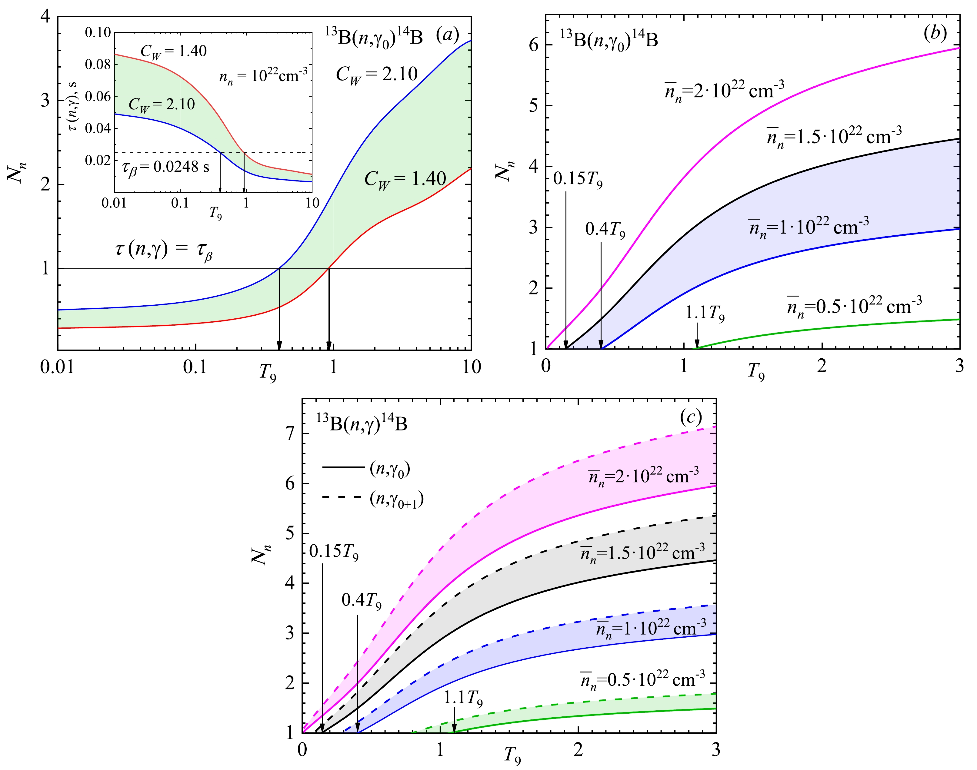
Figure 8. (color online) Number of captured neutrons Nn dependence on T9 conditioned by the neutron number density
$ {\bar n_n} $ . (a)$ {\bar n_n} $ = 1022 cm -3. The band corresponds to the reaction rates in Fig. 7. The insert shows the neutron capture time$ \tau (n,\gamma ). $ (b) Illustration of the ignition T9 values depending on the neutron number density$ {\bar n_n} $ . (c) Effect of the excited state: solid curves correspond to (n, γ0) capture to the GS; dashed curves correspond to the (n, γ0+1) total capture.The arrows indicate the equality
$ {\tau _\beta } = \tau (n,\gamma ) $ and reflect the equilibrium of the decay and capture processes, Nn = 1. The area under the dashed line holds$ \tau (n,\gamma ) < {\tau _\beta } $ , which means that the number of neutrons that interact with 13B is Nn > 1, as shown in the main field of Fig. 8 (a). We may conclude that at temperatures of T9 on the right of the arrows, the process (n, γ) is faster compared with β-decay. Therefore, the ignition of the 13B(n, γ0)14B reaction occurs at T9 ≥ 0.4 in the case of the reaction rate shown by the upper curve (CW = 2.10) in Fig. 7 (a) and at T9 ≥ 0.9 in the case of the low red curve (CW = 1.40).Figure 8 (b) shows the correlation between the variation in the neutron density and ignition temperature T9, i.e., for higher
$ {\bar n_n} $ , a lower T9 is needed to provide the number of (n, γ0) capture acts Nn > 1.Figure 8 (c) illustrates the same regularities, but we find a very specific feature. Fig. 7 (b) shows no essential input of the (n, γ1) process, playing the role of reaction rate correction, but its inclusion when considering neutron capture time
$\tau (n,{\gamma _{0 + 1}})$ leads to the noticeable shift in ignition points to the lower edge of the T9 scale:$ 0.15{T_9} \to 0.1{T_9}\, $ $ ({\bar n_n} = 1.5 \cdot {10^{22}} $ cm–3);$ 0.4{T_9} \to 0.3{T_9} $ ($ {\bar n_n} = 1 \cdot {10^{22}} $ cm–3);$ 1.1{T_9} \to 0.8{T_9} $ ($ {\bar n_n} = 0.5 \cdot {10^{22}} $ cm–3). Therefore, even a slight increase in reaction rate gives feedback to the occurrence of the 13B(n, γ0+1)14B reaction. There are no temperature constraints at high neutron density$ {\bar n_n} > 2 \cdot {10^{22}} $ .The T9 interval relevant to the start of the r-production of 14B may be defined at the present stage as 0.1 < T9 < 0.8 under neuron density matter conditions of 0.5·1022 cm−3 <
$ {\bar n_n} $ < 1.5·1022 cm−3. Based on these results, we compare the reaction rates of radiative neutron capture on 10-13B and 12-14C isotopes calculated within the same MPCM model formalism, as presented in Fig. 9.
Figure 9. (color online) Comparison of the neutron capture reaction rates on 10–13B and 12–14C isotopes calculated in the MPCM. 10B(n,γ)11B – blue solid curve [9], 11B(n, γ)12B – black solid curve [10, 11], 12B(n, γ)13B – pale blue band [12], 13B(n, γ)14B – pale green band (present calculations), 12C(n, γ)13C – blue dashed curve [13], 13C(n, γ)14C – red dashed curve [14], 14C(n, γ)15C – green dashed curve (unpublished). Additional details are provided in Table 5.
It is natural that the production of isotopes with mass number A following A-1 provides the continuation of the neutron-induced sequence if the previous reaction rate is comparable to or prevailed over by the next one. This regularity for the 10–13B isotopes is observed directly at temperatures of ~ 0.05 – 0.3T9, which overlaps with the window for 14B production. The gaps at low and high T9 in the case of the 11B(n, γ)12B reaction rate are not worrying because the isotope 11B is stable and may be accumulated.
We now complement the comparative analysis of the boron chain with information from Table 5. A correlation between the threshold energies Eth in the boron channels and the reaction rates at ultra-low T9 is observed, i.e., a higher Eth results in a higher reaction rate. The thermal cross-sections for odd-odd 10,12B isotopes are nearly an order larger than
${\sigma _{\rm therm}}$ of the odd-even 11,13B. We can observe these relationships for the reaction rates in Fig. 9, except at the temperature interval ~ 0.02 – 1T9 for the 11B(n, γ0+1+2+3+4)12B reaction, where the rate essentially increases owing to the large number of resonances in this channel. Moreover, the calculated${\sigma _{\rm therm}}$ for 11B(n, γ)12B shows excellent agreement with the measured value (see details in Refs. [10, 11]), and we interpret this result as the substantiation of the obtained${\sigma _{\rm therm}}$ for 13B(n, γ)14B in this study.Reaction Threshold energy Eth/MeV Included bound states Included resonances ${\sigma _{\rm therm} }$ /mb

Ref. 10B(n,γ)11B 11.4541 (n,γ0+2+3+4+9) 6+8P5/2, 6+8D5/2, 6+8D7/2 405 [9] 11B(n,γ)12B 3.3700 (n,γ0+1+2+3+4) 3+5P2, 3+5D1(I), 3+5D2, 3+5D3, 3+5D1(II), 5F1(I), 3+5F3(I), 5F1(II) 10.6 [10,11] 12B(n,γ)13B 4.8780 (n,γ0) 4D1/2, 4D5/2, 4P5/2 176 and 285 [12] 13B(n,γ)14B 0.9700 (n,γ0+1) 3+5P1 5.1 – 8.9 present 12C(n,γ)13C 4.9464 (n,γ0+1+2+3) 2D3/2 3.4 – 3.9 [13] 13C(n,γ)14C 8.1765 (n,γ0+1+2) 2P1/2 1.50 [14] 14C(n,γ)15C 1.2181 (n,γ0+1) 2P3/2 5·10-6 − Table 5. Overview of radiative neutron capture reactions on 10–13B and 12–14C isotopes calculated in the MPCM.
The isobar-analog channels 13B(n, γ)14B and 13C(n, γ)14C lead to the formation of 14C either via 14B β-decay or direct radiative neutron capture on 13C. Fig. 9 shows that at temperatures below 0.3T9, the boron channel rate exceeds the carbon one and decreases in the range ~ 0.3 – 3T9, and at T9 > 3, the reaction rates in both channels become close. Consequently, we may conclude that both 14C production processes exhibit comparable efficiency.
-
The total cross sections of the 13B(n, γ0+1)14B reaction are calculated in the MPCM based on the E1 and M1 transitions from 10-2 eV to 5 MeV. We prove that the strong sensitivity of the cross sections to the asymptotic constant CW provides an appropriate long-range dependence of the radial bound S wave functions; thus, a larger CW results in larger absolute values of cross-sections. The role of the FS in the calculated spectrum turned out to be insignificant.
The E1 transitions provides the background of the cross-section owing to the capture from the non-resonance 3+5P2, 5P3, and 3P0 waves, and the resonant 3+5P1 wave in the initial channel reveals the resonance structure of the cross-section at ~ 300 keV.
The M1 transition occurs via the S scattering wave and contributes predominantly to the thermal cross-sections. The variation in CW = 1.4 – 2.4 gives the range of
${\sigma _{\rm therm}}$ = 5.1 – 8.9 mb. These${\sigma _{\rm therm}}$ values have not ever been estimated in theory, which may be important for researchers.The reaction rates of the 13B(n, γ0+1)14B process exhibit the same dependence on the asymptotic constant CW and the relative contributions of the (n, γ0) and (n, γ1) channels. The results of MPCM calculations differ cardinally from those of Rauscher et al. [8] across the entire T9 range. Therefore, we conclude that the present data on the reaction rates substantiate the role of the 13B(n, γ0+1)14B reaction in boron-carbon-nitrogen chains, i.e., this is not the break-point of the boron sequence.
To support our conclusion, we estimate the relationship between the mean lifetime of 13B β decay τβ and neutron capture time
$ \tau (n,\gamma ) $ . The temperature window for the ignition of 14B r-production, 0.1 – 0.8T9, related to the neutron densities$ {\bar n_n} $ = 5 1021 – 1.5 1022 cm−3 is determined, whereas at$ {\bar n_n} $ > 1.5 1022 cm−3, there are no temperature limits. We demonstrate that the preferences for the 13B(n, γ0+1)14B reaction directly depend on the reaction rate values; the larger the$ \left\langle {{\sigma _{n,\gamma }}v} \right\rangle $ values, the shorter the neutron capture time$ \tau (n,\gamma ). $ We foresee the following factors increasing the reaction rate. The inclusion of the D-component into the bound GS (its weight is estimated today at ~ 17%) may enhance the input of the 1+ resonance to the E1 capture cross-section at 305 keV. The role of the transitions shown inFig. 2 but not considered in the present study may be evaluated; as an example, the inclusion of a rather weak (n, γ1) process leads to the narrowing of the ignition temperature interval. Another problem concerns the determination of 3π level parity at Ex = 4.06 MeV. If π = +1, the additional E1 transition may occur. In the case of π = −1, the E2 transition may reveal interference effects with the 3- state at Ex = 1.38 MeV.
The unique experimental results on the Coulomb dissociation of 14B [17], converted into the cross-section of the 13B(n, γ)14B reaction, remain preliminary and are not complete with estimated uncertainties.
We assume that our results on the reaction rate of 13B(n, γ)14B may change the perspective expressed in Ref. [7] on its minor impact on heavy element production. The present calculations are predictive and estimative to substantiate the performance of new experiments on the neutron capture on 13B and give a model estimation of the reaction rate of the synthesis of the 14B isotope in the n13B channel for the first time.
-
To assess reaction rate calculation accuracy, we evaluate the impact of the integration parameters on the calculated reaction rate (10). In addition, we study the influence of the integration method. The integration options we consider are the Simpson method (second order, m = 2) [43] and Milne method (fourth order, m = 4) [44].
Figure B1 shows the effect of changing Emax from 1 to 7 MeV at a constant step Estep = 0.25 keV using the Simpson method (panel a), and the dependence of the reaction rate on Estep varies from 0.1 keV to 1 keV at a constant Emax = 5 MeV (panel b).
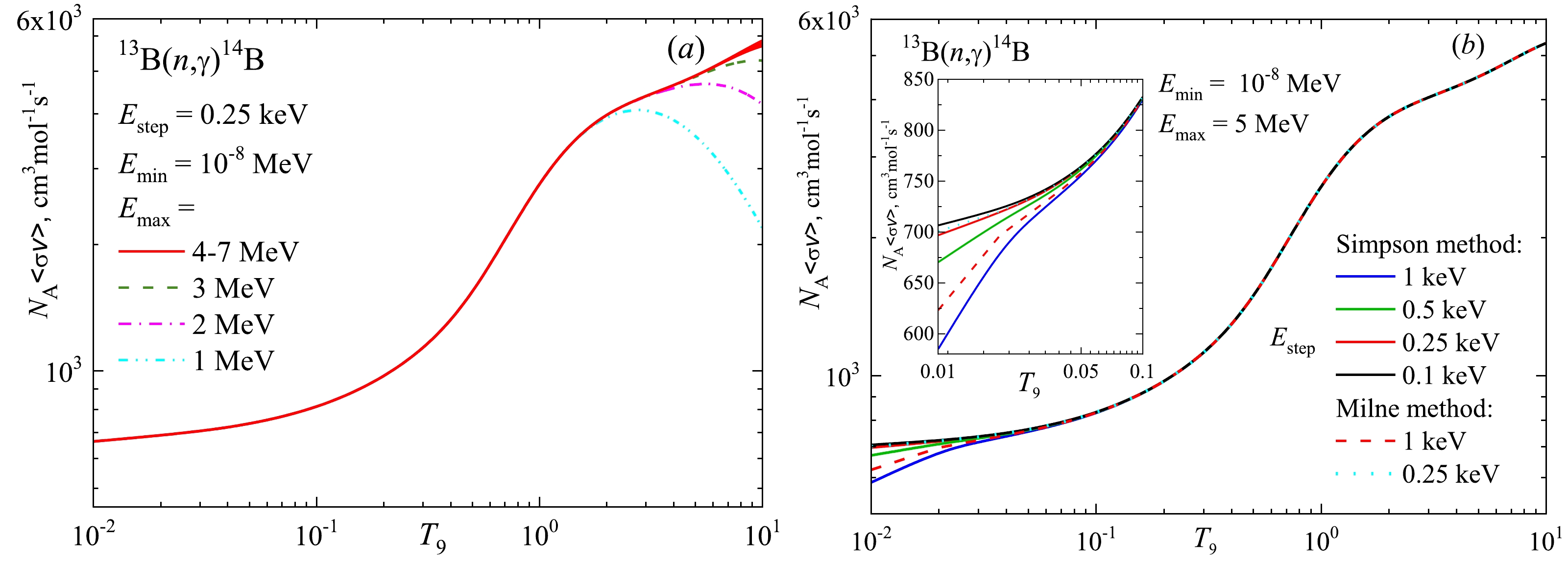
Figure B1. (color online) Dependence of the shape of the reaction rate on the integration procedure in expression (10). The lower integration limit Emin = 10–8 MeV. (a) Variation in Emax in the range of 1 MeV to 7 MeV at a constant Estep = 0.25 keV calculated using the Simpson method. (b) Variation in Estep in the range of 0.1 keV to 1 keV at a constant Emax of 5 MeV calculated using the Simpson and Milne methods.
When changing Emax, the shape of the reaction rate at high temperatures does not practically change at Emax ≥ 4 MeV. In the region of low temperature at Estep ≤ 0.25 keV, the shape of the reaction rate is virtually unchanged. In this study, we assume Emax = 5 MeV and an integration step Estep of 0.25 keV.
We also test the Milne method [44] with a uniform grid, assuming Emin = 0, the next point is at the first step of energy integration, and Emax = 4 MeV. Figure B1 (b) shows the results at Estep = 1 keV (red dashed curve) and Estep = 0.25 keV (blue dotted curve). At Estep = 0.25 keV, the calculation result does not depend on the method for calculating the integral of the reaction rate, but Milne's method works faster.
Estimation of radiative capture 13B(n, γ0+1)14B reaction rate in the modified potential cluster model
- Received Date: 2023-06-21
- Available Online: 2023-10-15
Abstract: We discuss current attempts to employ the modified potential cluster model to describe the available experimental data on the 13B(n, γ0+1)14B total cross-sections. The estimated results of the M1 and E1 transitions from the n13B scattering states to the ground and first excited states of 14B are presented. The 1st resonance at Ex = 1. 275 MeV (1+) is revealed in both the cross-section and reaction rate. Within the variation in the asymptotic constant, a thermal cross-section interval of 5.1 – 8.9 mb is proposed. Based on the theoretical total cross-sections at energies of 0.01 eV to 5 MeV, we calculate the reaction rate in the temperature range of 0.01 to 10T9. The ignition T9 values of the 13B(n, γ0+1)14B reaction depending on a neutron number density


 DownLoad: