


 Abstract
 HTML
HTML Reference
 Related
 PDF
PDF


-
In ultra-relativistic collisions of nuclei at both the Relativistic Heavy Ion Collider (RHIC) [1−4] and Large Hadron Collider (LHC) [5−8], a hot and dense system of strongly interacting quarks and gluons, known as “quark-gluon plasma” (QGP), is created. One of the key observables used to study the properties of QGP is the anisotropic collective flow, quantified by Fourier harmonics
$ {v_n} $ . Many methods have been developed to measure these harmonics [9−11]. One such method, the method of cumulants based on multi-particle correlations [12, 13], enables the suppression of short-range correlations arising from jets and resonance decays and then reveals a genuine collectivity arising from the expansion of QGP. The Q-cumulant method [14] is an improved version of the initial cumulant method. Recently, Q-cumulants were employed to examine hydrodynamics predictions in Ref. [15] based on the ratio of the differences between adjacent cumulants [16]. This analysis, performed using CMS data, indicated the necessity of introducing moments higher than skewness to describe the finer details of the elliptic flow$ {v_2} $ distribution. To do so, higher-order cumulants must be calculated. In this paper, we present a way of determining the expressions required to calculate higher-order cumulants.Sec. II of the paper gives the basic quantities used in the Q-cumulant method. Sec. III presents the foundation of the method within a finite-dimensional vector space. Sec. IV shows the results along with applications of the method to simple cases. Using toy models to demonstrate the capabilities of the method in Sec. V, and a summary is given in Sec. VI. Tables that summarize the coefficients needed to express the cumulants up to the 14-th order can be found in the appendix.
-
The general formalism of cumulants, for the purpose of flow measurements, was first used in Refs. [12−14], in which cumulants were expressed in terms of the moments of the magnitude of the corresponding flow vector. Such a cumulant method is systematically biased owing to the trivial effects of same particle autocorrelations. To avoid the computationally expensive “nested loops” used to remove autocorrelations in the measurements of multi-particle azimuthal correlations, Refs. [12−14] proposed an alternative method based on the use of generating functions. An improved cumulant method, Q-cumulants [14], allows, in principle, for fast and exact calculation of all multi-particle cumulants. However, in practice, the determination of the analytical expressions for multi-particle cumulants, which involve the azimuthal correlations of more than eight particles, is challenging.
Q-cumulants are built upon analytical expressions for multi-particle azimuthal correlations in terms of flow vectors Q, with
$ {Q_n} = \sum\limits_{j = 1}^M {{{\text{e}}^{in{\varphi _j}}}} , $

(1) evaluated at different orders of Fourier harmonics, n. Here, M is the multiplicity or number of particles in an event, and φj denotes the azimuthal angle of the j-th particle measured in a fixed coordinate system in the laboratory. The method involves the decomposition of the 2m-th power of the magnitude of the flow vector, |Qn|2m,
$ {\left| {{Q_n}} \right|^{2m}} = \sum\limits_{{j_1}, \ldots ,{j_{2m}} = 1}^M {{{\text{e}}^{in\left( {{\varphi _{{j_1}}} + \ldots + {\varphi _{{j_m}}} - {\varphi _{{j_{m + 1}}}} - \ldots - {\varphi _{{j_{2m}}}}} \right)}}} , $

(2) into (off diagonal) terms with 2m, 2m-1, … different indices up to the term where all 2m indices are equal (diagonal term). The first term, with 2m different indices, of decomposition is proportional to the 2m-particle azimuthal correlations
$ \left\langle {2m} \right\rangle $ ,$ \sum\limits_{{j_1} \ne \ldots \ne {j_{2m}} = 1}^M {{{\text{e}}^{in\left( {{\varphi _{{j_1}}} + \ldots + {\varphi _{{j_m}}} - {\varphi _{{j_{m + 1}}}} - \ldots - {\varphi _{{j_{2m}}}}} \right)}}} \equiv {P_{M,2m}} \cdot \left\langle {2m} \right\rangle , $

(3) where
$ {P_{M,2m}} $ is the number of distinct 2m-particle combinations one can form for an event with multiplicity M:$ {P_{M,2m}} = \frac{{M!}}{{(M - 2m)!}} . $

(4) In the case of full decomposition, |Qn|2m is expressed in readily calculable terms of powers of the flow vector given with Eq. (1) along with the anticipated 2m-particle azimuthal correlations introduced in Eq. (3). A thorough derivation with detailed examples is presented in Ref. [17]. The analytical decomposition of |Qn|2m for m > 4, however, becomes tedious.
In this paper, we present a numerical method for the decomposition of |Qn|2m that enables us, with the use of modern computers, to easily obtain analytical expressions for multi-particle azimuthal correlations of higher orders.
-
The full decomposition of |Qn|2m is divided into appropriate sets (or multisets in the case of repeated elements) of azimuthal angles that lead to the partial Bell polynomials or their generalization (in the case of multisets). In the derivation, some parts of the Bell polynomials must be expressed through lower-order multi-particle azimuthal correlations. This change of side in the expression causes a sign change of the corresponding term, resulting in the coefficients of the partial Bell polynomials in the final form of the 2m-particle azimuthal correlations being positive or negative integers. For example, in the case of m = 2, the four-particle azimuthal correlations might be presented as a linear combination of the corresponding Q-vector terms,
$\begin{aligned}[b] {P_{M,4}}\left\langle 4 \right\rangle =& + 1{\left| {{Q_n}} \right|^4} - 2{\rm Re} \left[ {{Q_{2n}}Q_n^ * Q_n^ * } \right] + 1{\left| {{Q_{2n}}} \right|^2} \\&- 4\left( {M - 2} \right){\left| {{Q_n}} \right|^2} + 2M\left( {M - 3} \right) , \end{aligned}$

(5) with the corresponding integer coefficients (+1, –2, +1, −4, +2) in front of each of the terms.
The same holds true for all 2m-particle correlations but with different sets of integer coefficients. This fact inspires us to calculate all these integer coefficients by solving an appropriate system of algebraic equations.
The 2m-particle correlations
$ \left\langle {2m} \right\rangle $ may be considered members of a finite-dimensional vector space Vd, where$ d = \dfrac{1}{2}\displaystyle\sum\limits_{l = 0}^m {p(l)[p(l) + 1]} $ is a dimension of the vector space, and$ p(l) = \{ 1,\;1,\;2,\;5,\;7, \ldots \} $ is a partition function of a non-negative integer$ l = \{ 0,\;1,\;2,\;3,\;4, \ldots \} $ . In Vd, we may define a basis$ {B_{\left\langle {2m} \right\rangle }} = ({{\mathbf{e}}_1},{{\mathbf{e}}_2},{{\mathbf{e}}_3}, \ldots ,{{\mathbf{e}}_d}) $ , which enables us to present$ {P_{M,2m}}\left\langle {2m} \right\rangle $ as a linear combination of the basis vectors$ {{\mathbf{e}}_i} $ :$ {P_{M,2m}}\left\langle {2m} \right\rangle = {x_1}f_1^{(m,l)}{{\mathbf{e}}_1} + {x_2}f_2^{(m,l)}{{\mathbf{e}}_2} + \ldots + {x_d}f_d^{(m,l)}{{\mathbf{e}}_d} , $

(6) where x1, x2, … are unknown integer numbers that must be obtained, and
$ f_i^{(m,l)} $ are known integer functions of the multiplicity M. The left side of Eq. (6) can be calculated directly from Eq. (3) only in case of low multiplicity because this is computationally manageable. The d unknown integer numbers,$ {x_1},{x_2}, \ldots ,{x_d} $ on the right hand side of Eq. (6) may be calculated numerically by solving the system of d linear algebraic equations presented in the next section. -
The full analytical determination of the basis
$ {B_{\left\langle {2m} \right\rangle }} $ is presented in Ref. [17] for$ m = 1, \ldots ,4 $ . However, in this paper, we show the straightforward determination of the basis using the method of mathematical induction, which enables easy calculation of the multi-particle azimuthal correlations of higher orders. First, it should be noted from simple inspection of the published results [14, 17] that each basis$ {B_{\left\langle {2m} \right\rangle }} $ contains the complete basis of the lower number (2m-2)-particle azimuthal correlations${B_{\left\langle {2m - 2} \right\rangle }}\subset {B_{\left\langle {2m} \right\rangle }}$ . For example, the basis of the 4-particle azimuthal correlations contains the complete basis of the 2-particle azimuthal correlations$ {B_{\left\langle 2 \right\rangle }} = \left( {1,{{\left| {{Q_n}} \right|}^2}} \right) $ and some additional basis vectors,$ {B_{\left\langle 4 \right\rangle }} = \left( {{B_{\left\langle 2 \right\rangle }},{{\left| {{Q_n}} \right|}^4},{\rm Re} ({Q_{2n}}Q_n^*Q_n^*),{{\left| {{Q_{2n}}} \right|}^2}} \right) . $

(7) Moreover, the basis
$ {B_{\left\langle 2 \right\rangle }} = \left( {{B_{\left\langle 0 \right\rangle }},{{\left| {{Q_n}} \right|}^2}} \right) $ might be considered an extension of the basis$ {B_{\left\langle 0 \right\rangle }} $ , with an additional basis vector$ {\left| {{Q_n}} \right|^2} $ . All additional vectors in the basis$ {B_{\left\langle {2l} \right\rangle }} $ form a subset l, whose dimension is$ d(l) = \dfrac{1}{2}p(l)\left[ {p(l) + 1} \right] $ . Thus, the problem of determining the basis$ {B_{\left\langle {2m} \right\rangle }} $ reduces to finding the subset l = m.We find that the subset l = m contains different compositions (products) of the flow vectors
$ {Q_{sub1}}{Q_{sub2}} \cdots $ , each with a subscript (sub1, sub2,…) that corresponds to the well-known “partition of the positive integer” m. For example, in the case of the 8-particle (2m = 8) azimuthal correlations, the subset l = 4 contains the following compositions of the flow vectors:$ \begin{array}{*{20}{c}} {\quad \quad \quad \,{Q_{1n}}{Q_{1n}}{Q_{1n}}{Q_{1n}}} \\ {\quad \quad \,{Q_{2n}}{Q_{1n}}{Q_{1n}}} \\ {\quad \,{Q_{2n}}{Q_{2n}}} \\ {\quad \,{Q_{3n}}{Q_{1n}}} \\ {{Q_{4n}}} \end{array}\quad \mathop \Leftarrow \limits^{} \quad \quad \left\{ {\begin{array}{*{20}{c}} 1&1&1&1 \\ 2&1&1&{} \\ 2&2&{}&{} \\ 3&1&{}&{} \\ 4&{}&{}&{} \end{array}} \right. , $

(8) where each composition contains subscripts that correspond to the partition of the integer 4.
Here, we use the convenient symbolic notation introduced in Refs. [14, 17],
$ {Q_{p \cdot n}} \equiv \sum\limits_{j = 1}^M {{{\rm e}^{p \cdot in{\varphi _j}}}} ,p \in \{ 1,2,3, \ldots \} . $

(9) To obtain all the basis vectors of the subset l = 4, each composition in (8) must be combined by the ordered composition of the complex conjugate vectors, as shown in the following pattern:

This pattern gives fifteen (p(4)[p(4)+1]/2 = 15) different combinations:
$ \begin{gathered} \begin{array}{*{20}{c}} {{Q_n}{Q_n}{Q_n}{Q_n}|Q_n^*Q_n^*Q_n^*Q_n^*} \\ {} \\ {} \\ {} \end{array}\quad \quad \begin{array}{*{20}{c}} {\;\;{\kern 1pt} {Q_{2n}}{Q_n}{Q_n}|Q_n^*Q_n^*Q_n^*Q_n^*} \\ {{Q_{2n}}{Q_n}{Q_n}|Q_{2n}^*Q_n^*Q_n^*} \\ {} \\ {} \end{array}\quad \quad \begin{array}{*{20}{c}} {\;\;\;\;{\kern 1pt} {\kern 1pt} {Q_{2n}}{Q_{2n}}|Q_n^*Q_n^*Q_n^*Q_n^*} \\ {\;\;{\kern 1pt} {Q_{2n}}{Q_{2n}}|Q_{2n}^*Q_n^*Q_n^*} \\ {{Q_{2n}}{Q_{2n}}|Q_{2n}^*Q_{2n}^*} \\ {} \end{array} \\ \begin{array}{*{20}{c}} {\;\;\;\;\;\;{Q_{3n}}{Q_n}|Q_n^*Q_n^*Q_n^*Q_n^*} \\ {\;\;\;{\kern 1pt} {Q_{3n}}{Q_n}|Q_{2n}^*Q_n^*Q_n^*} \\ {\;{Q_{3n}}{Q_n}|Q_{2n}^*Q_{2n}^*} \\ {{Q_{3n}}{Q_n}|Q_{3n}^*Q_n^*} \\ {} \end{array}\quad \quad \begin{array}{*{20}{c}} {\quad \quad \;\;{Q_{4n}}|Q_n^*Q_n^*Q_n^*Q_n^*} \\ {\quad \;\;\;{Q_{4n}}|Q_{2n}^*Q_n^*Q_n^*} \\ {\quad {\kern 1pt} {\kern 1pt} {Q_{4n}}|Q_{2n}^*Q_{2n}^*} \\ {\;\;\;{\kern 1pt} {Q_{4n}}|Q_{3n}^*Q_n^*} \\ {{Q_{4n}}|Q_{4n}^*} \end{array} \\ \end{gathered} $ 
(11) The real part of each of these additional vectors (11), together with the basis
$ {B_{\left\langle 6 \right\rangle }} $ , makes the complete basis of the 8-particle azimuthal correlations$ {B_{\left\langle 8 \right\rangle }} $ . This presentation of the composition of the flow vectors separated from the complex conjugate part by a vertical bar is inspired by the work of Ref. [14].The corresponding multiplying integer functions
$ {f^{(m,l)}} $ might also be obtained via mathematical induction. These integer functions are given by$ \begin{gathered} (M - 2l)\prod\limits_{j = m + l + 1}^{2m - 1} {(M - j)} ,\quad {\text{for}}\quad l = \{ 0,...,m - 2\} \\ M - 2l,\quad {\text{for}}\quad l = m - 1 \\ 1,\quad {\text{for}}\quad l = m \\ \end{gathered} . $

(12) For example, in the case of the 8-particle azimuthal correlations (m = 4),
$ {f^{(m = 4,l)}} = \left\{ \begin{aligned} M(M - 5)(M - 6)(M - 7),\quad {\text{for}}\quad l = 0 \\ (M - 2)(M - 6)(M - 7),\quad {\text{for}}\quad l = 1 \\ (M - 4)(M - 7),\quad {\text{for}}\quad l = 2 \\ (M - 6),\quad {\text{for}}\quad l = 3 \\ 1,\quad {\text{for}}\quad l = 4 \\ \end{aligned} \right. . $

(13) We list the integer functions and basis vectors for each of the 2m-particle azimuthal correlations (
$ m = 1,2, \ldots ,7 $ ) in the third and fourth columns, respectively, of Tables 1−7.$ i $ 

$ {x_i} $ 

$ f_i^{(m = 1,l)} $ 

Basis vectors l 1 −1 M 1 0 2 1 1 $ {Q_n}|Q_n^* $ 

1 Table 1. Coefficients, integer functions, and basis vectors for the calculation of the two-particle azimuthal correlations.
$ i $ 

$ {x_i} $ 

$ f_i^{(m = 2,l)} $ 

Basis vectors l 1 2 $ M(M - 3) $ 

1 0 2 −4 $ (M - 2) $ 

$ {Q_n}|Q_n^* $ 

1 3 1 1 $ {Q_n}{Q_n}|Q_n^*Q_n^* $ 

2 4 −2 1 $ {Q_{2n}}{{ }}|Q_n^*Q_n^* $ 

2 5 1 1 $ {Q_{2n}}{{ }}|{{ }}Q_{2n}^* $ 

2 Table 2. Coefficients, integer functions, and basis vectors for the calculation of the four-particle azimuthal correlations.
$ i $ 

$ {x_i} $ 

$ f_i^{(m = 3,l)} $ 

Basis vectors l 1 −6 $ M(M - 4)(M - 5) $ 

$ 1 $ 

0 2 18 $ (M - 2)(M - 5) $ 

$ {Q_n}|Q_n^* $ 

1 3 −9 $ (M - 4) $ 

$ {Q_n}{Q_n}|Q_n^*Q_n^* $ 

2 4 18 $ (M - 4) $ 

$ {Q_{2n}}{{ }}|Q_n^*Q_n^* $ 

2 5 −9 $ (M - 4) $ 

$ {Q_{2n}}{{ }}|{{ }}Q_{2n}^* $ 

2 6 1 1 $ {Q}_{n}{Q}_{n}{Q}_{n}�{|}{Q}_{n}^{*}{Q}_{n}^{*}{Q}_{n}^{*} $ 

3 7 −6 1 $ {Q_{2n}}{{ }}{Q_n}{{|}}Q_n^*Q_n^*Q_n^* $ 

3 8 9 1 $ {Q_{2n}}{{ }}{Q_n}{{|}}Q_n^*{{ }}Q_{2n}^* $ 

3 9 4 1 $ {Q_{3n}}{{ |}}Q_n^*Q_n^*Q_n^* $ 

3 10 −12 1 $ {Q_{3n}}{{ |}}Q_n^*{{ }}Q_{2n}^* $ 

3 11 4 1 $ {Q}_{3n}{ |}�����{ }{Q}_{3n}^{*} $ 

3 Table 3. Coefficients, integer functions, and basis vectors for the calculation of the six-particle azimuthal correlations.
$ i $ 

$ {x_i} $ 

$ f_i^{(m = 4,l)} $ 

Basis vectors l 1 24 $ M(M - 5)(M - 6)(M - 7) $ 

$ 1 $ 

0 2 −96 $ (M - 2)(M - 6)(M - 7) $ 

$ {Q_n}|Q_n^* $ 

1 3 72 $ (M - 4)(M - 7) $ 

$ {Q_n}{Q_n}|Q_n^*Q_n^* $ 

2 4 −144 $ (M - 4)(M - 7) $ 

$ {Q_{2n}}{{ }}|Q_n^*Q_n^* $ 

2 5 72 $ (M - 4)(M - 7) $ 

$ {Q_{2n}}{{ }}|{{ }}Q_{2n}^* $ 

2 6 −16 $ (M - 6) $ 

$ {Q}_{n}{Q}_{n}{Q}_{n}�{|}{Q}_{n}^{*}{Q}_{n}^{*}{Q}_{n}^{*} $ 

3 7 96 $ (M - 6) $ 

$ {Q_{2n}}{{ }}{Q_n}{{|}}Q_n^*Q_n^*Q_n^* $ 

3 8 −144 $ (M - 6) $ 

$ {Q_{2n}}{{ }}{Q_n}{{|}}Q_n^*{{ }}Q_{2n}^* $ 

3 9 −64 $ (M - 6) $ 

$ {Q_{3n}}{{ |}}Q_n^*Q_n^*Q_n^* $ 

3 10 192 $ (M - 6) $ 

$ {Q_{3n}}{{ |}}Q_n^*{{ }}Q_{2n}^* $ 

3 11 −64 $ (M - 6) $ 

$ {Q}_{3n}{ |}{ }{Q}_{3n}^{*} $ 

3 12 1 1 $ {Q_n}{Q_n}{Q_n}{Q_n}{{|}}Q_n^*Q_n^*Q_n^*Q_n^* $ 

4 13 −12 1 $ {Q_{2n}}{{ }}{Q_n}{Q_n}{{|}}Q_n^*Q_n^*Q_n^*Q_n^* $ 

4 14 36 1 $ {Q_{2n}}{{ }}{Q_n}{Q_n}{{|}}Q_n^*Q_n^*{{ }}Q_{2n}^* $ 

4 15 6 1 $ {Q_{2n}}{{ }}{Q_{2n}}{{ |}}Q_n^*Q_n^*Q_n^*Q_n^* $ 

4 16 −36 1 $ {Q_{2n}}{{ }}{Q_{2n}}{{ |}}Q_n^*Q_n^*{{ }}Q_{2n}^* $ 

4 17 9 1 $ {Q_{2n}}{{ }}{Q_{2n}}{{ | }}Q_{2n}^*{{ }}Q_{2n}^* $ 

4 18 16 1 $ {Q_{3n}}{{ }}{Q_n}{{|}}Q_n^*Q_n^*Q_n^*Q_n^* $ 

4 19 −96 1 $ {Q_{3n}}{{ }}{Q_n}{{|}}Q_n^*Q_n^*{{ }}Q_{2n}^* $ 

4 20 48 1 $ {Q_{3n}}{{ }}{Q_n}{{| }}Q_{2n}^*{{ }}Q_{2n}^* $ 

4 21 64 1 $ {Q_{3n}}{{ }}{Q_n}{{|}}Q_n^*{{ }}Q_{3n}^* $ 

4 22 −12 1 $ {Q_{4n}}{{ |}}Q_n^*Q_n^*Q_n^*Q_n^* $ 

4 23 72 1 $ {Q_{4n}}{{ |}}Q_n^*Q_n^*{{ }}Q_{2n}^* $ 

4 24 −36 1 $ {Q_{4n}}{{ | }}Q_{2n}^*{{ }}Q_{2n}^* $ 

4 25 −96 1 $ {Q_{4n}}{{ |}}Q_n^*{{ }}Q_{3n}^* $ 

4 26 36 1 $ {Q}_{4n}{ |}{ }{Q}_{4n}^{*} $ 

4 Table 4. Coefficients, integer functions, and basis vectors for the calculation of the eight-particle azimuthal correlations.
$ i $ 

$ {x_i} $ 

$ f_i^{(m = 5,l)} $ 

Basis vectors l 1 −120 $ M(M - 6)(M - 7)(M - 8)(M - 9) $ 

$ 1 $ 

0 2 600 $ (M - 2)(M - 7)(M - 8)(M - 9) $ 

$ {Q_n}|Q_n^* $ 

1 3 −600 $ (M - 4)(M - 8)(M - 9) $ 

$ {Q_n}{Q_n}|Q_n^*Q_n^* $ 

2 4 1200 $ (M - 4)(M - 8)(M - 9) $ 

${Q_{2n} }|Q_n^*Q_n^*$ 

2 5 −600 $ (M - 4)(M - 8)(M - 9) $ 

$ {Q_{2n}}{}|{}Q_{2n}^* $ 

2 6 200 $ (M - 6)(M - 9) $ 

$ {Q}_{n}{Q}_{n}{Q}_{n}�{|}{Q}_{n}^{*}{Q}_{n}^{*}{Q}_{n}^{*} $ 

3 7 −1200 $ (M - 6)(M - 9) $ 

$ {Q_{2n}}{}{Q_n}{{|}}Q_n^*Q_n^*Q_n^* $ 

3 8 1800 $ (M - 6)(M - 9) $ 

$ {Q_{2n}}{}{Q_n}{{|}}Q_n^*{}Q_{2n}^* $ 

3 9 800 $ (M - 6)(M - 9) $ 

$ {Q_{3n}}{{ |}}Q_n^*Q_n^*Q_n^* $ 

3 10 −2400 $ (M - 6)(M - 9) $ 

$ {Q_{3n}}{{ |}}Q_n^*{}Q_{2n}^* $ 

3 11 800 $ (M - 6)(M - 9) $ 

$ {Q}_{3n}{ |}{Q}_{3n}^{*} $ 

3 12 −25 $ (M - 8) $ 

$ {Q_n}{Q_n}{Q_n}{Q_n}{{|}}Q_n^*Q_n^*Q_n^*Q_n^* $ 

4 13 300 $ (M - 8) $ 

$ {Q_{2n}}{}{Q_n}{Q_n}{{|}}Q_n^*Q_n^*Q_n^*Q_n^* $ 

4 14 −900 $ (M - 8) $ 

$ {Q_{2n}}{}{Q_n}{Q_n}{{|}}Q_n^*Q_n^*{}Q_{2n}^* $ 

4 15 −150 $ (M - 8) $ 

$ {Q_{2n}}{}{Q_{2n}}{{ |}}Q_n^*Q_n^*Q_n^*Q_n^* $ 

4 16 900 $ (M - 8) $ 

$ {Q_{2n}}{}{Q_{2n}}{{ |}}Q_n^*Q_n^*{}Q_{2n}^* $ 

4 17 −225 $ (M - 8) $ 

$ {Q_{2n}}{}{Q_{2n}}{{ | }}Q_{2n}^*{}Q_{2n}^* $ 

4 18 −400 $ (M - 8) $ 

$ {Q_{3n}}{}{Q_n}{{|}}Q_n^*Q_n^*Q_n^*Q_n^* $ 

4 19 2400 $ (M - 8) $ 

$ {Q_{3n}}{}{Q_n}{{|}}Q_n^*Q_n^*{}Q_{2n}^* $ 

4 20 −1200 $ (M - 8) $ 

$ {Q_{3n}}{}{Q_n}{{| }}Q_{2n}^*{}Q_{2n}^* $ 

4 21 −1600 $ (M - 8) $ 

$ {Q_{3n}}{}{Q_n}{{|}}Q_n^*{}Q_{3n}^* $ 

4 22 300 $ (M - 8) $ 

$ {Q_{4n}}{{ |}}Q_n^*Q_n^*Q_n^*Q_n^* $ 

4 23 −1800 $ (M - 8) $ 

$ {Q_{4n}}{{ |}}Q_n^*Q_n^*{}Q_{2n}^* $ 

4 24 900 $ (M - 8) $ 

$ {Q_{4n}}{{ | }}Q_{2n}^*{}Q_{2n}^* $ 

4 25 2400 $ (M - 8) $ 

$ {Q_{4n}}{{ |}}Q_n^*{}Q_{3n}^* $ 

4 26 −900 $ (M - 8) $ 

$ {Q}_{4n}{ |}{ }{Q}_{4n}^{*} $ 

4 27 1 1 $ {Q_n}{Q_n}{Q_n}{Q_n}{Q_n}{{|}}Q_n^*Q_n^*Q_n^*Q_n^*Q_n^* $ 

5 28 −20 1 $ {Q_{2n}}{}{Q_n}{Q_n}{Q_n}{{|}}Q_n^*Q_n^*Q_n^*Q_n^*Q_n^* $ 

5 29 100 1 $ {Q_{2n}}{}{Q_n}{Q_n}{Q_n}{{|}}Q_n^*Q_n^*Q_n^*{}Q_{2n}^* $ 

5 30 30 1 $ {Q_{2n}}{}{Q_{2n}}{}{Q_n}{{|}}Q_n^*Q_n^*Q_n^*Q_n^*Q_n^* $ 

5 31 −300 1 $ {Q_{2n}}{}{Q_{2n}}{}{Q_n}{{|}}Q_n^*Q_n^*Q_n^*{}Q_{2n}^* $ 

5 32 225 1 ${Q_{2n} }{Q_{2n} }{ }{Q_n}{{|} }Q_n^*{ }Q_{2n}^*{ }Q_{2n}^*$ 

5 33 40 1 ${Q_{3n} }{Q_n}{Q_n}{{|} }Q_n^*Q_n^*Q_n^*Q_n^*Q_n^*$ 

5 34 −400 1 ${Q_{3n} }{Q_n}{Q_n}{{|} }Q_n^*Q_n^*Q_n^*{ }Q_{2n}^*$ 

5 35 600 1 ${Q_{3n} }{Q_n}{Q_n}{{|} }Q_n^*{ }Q_{2n}^*{ }Q_{2n}^*$ 

5 36 400 1 ${Q_{3n} }{Q_n}{Q_n}{{|} }Q_n^*Q_n^*{ }Q_{3n}^*$ 

5 37 −40 1 ${Q}_{3n}{Q}_{2n}{|}{Q}_{n}^{*}{Q}_{n}^{*}{Q}_{n}^{*}{Q}_{n}^{*}{Q}_{n}^{*}$ 

5 38 400 1 ${Q}_{3n}{Q}_{2n}{|}{Q}_{n}^{*}{Q}_{n}^{*}{Q}_{n}^{*}{Q}_{2n}^{*}$ 

5 39 −600 1 ${Q}_{3n}{Q}_{2n}{|}{Q}_{n}^{*}{Q}_{2n}^{*}{Q}_{2n}^{*}$ 

5 40 −800 1 ${Q}_{3n}{Q}_{2n}�{|}{Q}_{n}^{*}{Q}_{n}^{*}{Q}_{3n}^{*}$ 

5 41 400 1 ${Q}_{3n}{Q}_{2n}{|}{Q}_{2n}^{*}{Q}_{3n}^{*}$ 

5 Continued on next page Table 5. Coefficients, integer functions, and basis vectors for the calculation of the ten-particle azimuthal correlations.
$ i $ 

$ {x_i} $ 

$ f_i^{(m = 6,l)} $ 

Basis vectors l 1 720 $ M(M - 7)(M - 8)(M - 9)(M - 10)(M - 11) $ 

$ 1 $ 

0 2 −4320 $ (M - 2)(M - 8)(M - 9)(M - 10)(M - 11) $ 

$ {Q_n}|Q_n^* $ 

1 3 5400 $ (M - 4)(M - 9)(M - 10)(M - 11) $ 

$ {Q_n}{Q_n}|Q_n^*Q_n^* $ 

2 4 −10800 $ (M - 4)(M - 9)(M - 10)(M - 11) $ 

$ {Q_{2n}}{{ }}|Q_n^*Q_n^* $ 

2 5 5400 $ (M - 4)(M - 9)(M - 10)(M - 11) $ 

$ {Q_{2n}}{{ }}|{{ }}Q_{2n}^* $ 

2 6 −2400 $ (M - 6)(M - 10)(M - 11) $ 

$ {Q}_{n}{Q}_{n}{Q}_{n}{|}{Q}_{n}^{*}{Q}_{n}^{*}{Q}_{n}^{*} $ 

3 7 14400 $ (M - 6)(M - 10)(M - 11) $ 

$ {Q_{2n}}{{ }}{Q_n}{{|}}Q_n^*Q_n^*Q_n^* $ 

3 8 −21600 $ (M - 6)(M - 10)(M - 11) $ 

$ {Q_{2n}}{{ }}{Q_n}{{|}}Q_n^*{{ }}Q_{2n}^* $ 

3 9 −9600 $ (M - 6)(M - 10)(M - 11) $ 

${Q_{3n} }{{|} }Q_n^*Q_n^*Q_n^*$ 

3 10 28800 $ (M - 6)(M - 10)(M - 11) $ 

$ {Q_{3n}}{{ |}}Q_n^*{{ }}Q_{2n}^* $ 

3 11 −9600 $ (M - 6)(M - 10)(M - 11) $ 

${Q}_{3n}{|}{}{Q}_{3n}^{*}$ 

3 12 450 $ (M - 8)(M - 11) $ 

$ {Q_n}{Q_n}{Q_n}{Q_n}{{|}}Q_n^*Q_n^*Q_n^*Q_n^* $ 

4 13 −5400 $ (M - 8)(M - 11) $ 

$ {Q_{2n}}{{ }}{Q_n}{Q_n}{{|}}Q_n^*Q_n^*Q_n^*Q_n^* $ 

4 14 16200 $ (M - 8)(M - 11) $ 

$ {Q_{2n}}{{ }}{Q_n}{Q_n}{{|}}Q_n^*Q_n^*{{ }}Q_{2n}^* $ 

4 15 2700 $ (M - 8)(M - 11) $ 

$ {Q_{2n}}{{ }}{Q_{2n}}{{ |}}Q_n^*Q_n^*Q_n^*Q_n^* $ 

4 16 −16200 $ (M - 8)(M - 11) $ 

$ {Q_{2n}}{{ }}{Q_{2n}}{{ |}}Q_n^*Q_n^*{{ }}Q_{2n}^* $ 

4 17 4050 $ (M - 8)(M - 11) $ 

$ {Q_{2n}}{{ }}{Q_{2n}}{{ | }}Q_{2n}^*{{ }}Q_{2n}^* $ 

4 18 7200 $ (M - 8)(M - 11) $ 

$ {Q_{3n}}{{ }}{Q_n}{{|}}Q_n^*Q_n^*Q_n^*Q_n^* $ 

4 19 −43200 $ (M - 8)(M - 11) $ 

$ {Q_{3n}}{{ }}{Q_n}{{|}}Q_n^*Q_n^*{{ }}Q_{2n}^* $ 

4 20 21600 $ (M - 8)(M - 11) $ 

$ {Q_{3n}}{{ }}{Q_n}{{| }}Q_{2n}^*{{ }}Q_{2n}^* $ 

4 21 28800 $ (M - 8)(M - 11) $ 

$ {Q_{3n}}{{ }}{Q_n}{{|}}Q_n^*{{ }}Q_{3n}^* $ 

4 22 −5400 $ (M - 8)(M - 11) $ 

$ {Q_{4n}}{{ |}}Q_n^*Q_n^*Q_n^*Q_n^* $ 

4 23 32400 $ (M - 8)(M - 11) $ 

$ {Q_{4n}}{{ |}}Q_n^*Q_n^*{{ }}Q_{2n}^* $ 

4 24 −16200 $ (M - 8)(M - 11) $ 

$ {Q_{4n}}{{ | }}Q_{2n}^*{{ }}Q_{2n}^* $ 

4 25 −43200 $ (M - 8)(M - 11) $ 

$ {Q_{4n}}{{ |}}Q_n^*{{ }}Q_{3n}^* $ 

4 Continued on next page Table 6. Coefficients, integer functions, and basis vectors for the calculation of the twelve-particle azimuthal correlations.
Now, we have all the necessary quantities to form the system of linear equations to obtain all the unknown coefficients for each of the 2m-particle azimuthal correlations:
$ \begin{gathered} {\left( {\sum\limits_{{j_1} \ne \ldots \ne {j_{2m}} = 1}^M {{{\text{e}}^{in\left( {{\varphi _{{j_1}}} + \ldots + {\varphi _{{j_m}}} - {\varphi _{{j_{m + 1}}}} - \ldots - {\varphi _{{j_{2m}}}}} \right)}}} } \right)_{{\text{event}}1}} = {x_1}{\left( {f_1^{(m,l)}{{\mathbf{e}}_1}} \right)_{{\text{event}}1}} + {x_2}{\left( {f_2^{(m,l)}{{\mathbf{e}}_2}} \right)_{{\text{event}}1}} + \ldots + {x_d}{\left( {f_d^{(m,l)}{{\mathbf{e}}_d}} \right)_{{\text{event}}1}} \\ {\left( {\sum\limits_{{j_1} \ne \ldots \ne {j_{2m}} = 1}^M {{{\text{e}}^{in\left( {{\varphi _{{j_1}}} + \ldots + {\varphi _{{j_m}}} - {\varphi _{{j_{m + 1}}}} - \ldots - {\varphi _{{j_{2m}}}}} \right)}}} } \right)_{{\text{event}}2}} = {x_1}{\left( {f_1^{(m,l)}{{\mathbf{e}}_1}} \right)_{{\text{event}}2}} + {x_2}{\left( {f_2^{(m,l)}{{\mathbf{e}}_2}} \right)_{{\text{event}}2}} + \ldots + {x_d}{\left( {f_d^{(m,l)}{{\mathbf{e}}_d}} \right)_{{\text{event}}2}} \\ \vdots \quad \quad \quad \quad \quad \quad = \quad \quad \quad \quad \quad \quad \quad \quad \quad \vdots \\ \\ {\left( {\sum\limits_{{j_1} \ne \ldots \ne {j_{2m}} = 1}^M {{{\text{e}}^{in\left( {{\varphi _{{j_1}}} + \ldots + {\varphi _{{j_m}}} - {\varphi _{{j_{m + 1}}}} - \ldots - {\varphi _{{j_{2m}}}}} \right)}}} } \right)_{{\text{event}}d}} = {x_1}{\left( {f_1^{(m,l)}{{\mathbf{e}}_1}} \right)_{{\text{event}}d}} + {x_2}{\left( {f_2^{(m,l)}{{\mathbf{e}}_2}} \right)_{{\text{event}}d}} + \ldots + {x_d}{\left( {f_d^{(m,l)}{{\mathbf{e}}_d}} \right)_{{\text{event}}d}} \\ \end{gathered} , $ 
(14) To set a solvable system of Eq. (14), the multiplicity must be
$ M \geqslant 2m $ (otherwise, the system of equations cannot be formed). For example, the system of equations for the 2-particle azimuthal correlations is given by ($ M \geqslant 2 $ )$ \begin{gathered} {\left( {\sum\limits_{{j_1} \ne {j_2} = 1}^M {{{\text{e}}^{in\left( {{\varphi _{{j_1}}} - {\varphi _{{j_2}}}} \right)}}} } \right)_{{\text{event}}1}} = {x_1}{\left( {M \cdot 1} \right)_{{\text{event}}1}} + {x_2}{\left( {1 \cdot {{\left| {{Q_n}} \right|}^2}} \right)_{{\text{event}}1}} \\ {\left( {\sum\limits_{{j_1} \ne {j_2} = 1}^M {{{\text{e}}^{in\left( {{\varphi _{{j_1}}} - {\varphi _{{j_2}}}} \right)}}} } \right)_{{\text{event}}2}} = {x_1}{\left( {M \cdot 1} \right)_{{\text{event}}2}} + {x_2}{\left( {1 \cdot {{\left| {{Q_n}} \right|}^2}} \right)_{{\text{event}}2}} \\ \end{gathered} . $

(15) Note that in the sum on the left-hand side of Eq. (15), a complex number and its conjugate are included; hence, the sum is reduced to a real number. To set the system of Eq. (15), we randomly choose two sets of angles:
$ {\varphi _{{j_1}}} = {\text{0}}.400906 $ ,$ {\varphi _{{j_2}}} = - 2.{\text{84149}} $ ,$ {\varphi _{{j_3}}} = $ 1.98067 (multiplicity M = 3) for the first equation and$ {\varphi _{{j_1}}} = - {\text{1}}{\text{.32161}} $ ,$ \varphi _{j_2} = 2.75646 $ ,$ {\varphi _{j_3}} = 2.8089} $ ,$ {\varphi _{{j_4}}} = $ 1.59479,$ {\varphi _{{j_5}}} = {\text{1}}.13565 $ , (M = 5) for the second one. Then, the system of equations given by Eq. (15) for n = 2 becomes$ \begin{gathered} {{ - 1}}{\text{.992180682386965}} = {x_1} \cdot 3 + {x_2} \cdot {\text{1}}{\text{.007819317613035}} \\ {{ - 2}}{\text{.80896273559164}} = {x_1} \cdot 5 + {x_2} \cdot {\text{2}}{\text{.19103726440836}} \\ \end{gathered} . $

(16) Using the same sets of azimuthal angles for the Fourier harmonic n = 3, the system of Eq. (15) becomes
$ \begin{gathered} {{-2}}{\text{.502229604410126}} = {x_1} \cdot 3 + {x_2} \cdot {\text{0}}{\text{.497770395589874}} \\ {\text{2}}{\text{.85297668985644}} = {x_1} \cdot 5 + {x_2} \cdot {\text{7}}{\text{.85297668985644}} \\ \end{gathered} . $

(17) These two systems of linear equations are mutually different but both have the same solution:
$ {x_1} = - 1 $ ,$ {x_2} = 1 $ ; therefore, we fill the second column of Table 1 with the corresponding$ {x_i} $ values.The sets of azimuthal angles may be chosen randomly, as in the upper example. This should ensure that the calculated basis
$ {B_{\left\langle {2m} \right\rangle }} $ does not have collinear vectors; otherwise, the linear system of equations is not solvable.The calculated numbers that enter the system of Eqs. (16) and (17) should be given an appropriate number of significant digits for the obtained coefficients
$ {x_i} $ to be true integers. There are no criteria to determine the appropriate number of significant digits. We can use the ‘trial and error’ method to find the required number. Otherwise, the obtained$ {x_i} $ will not be integers, and the rounding of$ {x_i} $ might be problematic in the case of a large basis$ {B_{\left\langle {2m} \right\rangle }} $ . The limits of the application of this method depend on the number of significant digits by which the computer operates. We successfully apply the method up to the 14-th order of cumulants.The two-particle azimuthal correlation formula can be formed by simply reading the corresponding values from Table 1:
$ \left\langle 2 \right\rangle {P_{M,2}} = {x_1}f_1^{(m = 1,0)}1 + {x_2}f_2^{(m = 1,1)}{\rm Re} \left( {{Q_n}Q_n^*} \right) = - M + {\left| {{Q_n}} \right|^2} . $

(18) A similar table can be obtained for the four-particle azimuthal correlations using the solution of the corresponding linear system of equations.
This can also be easily rewritten as an appropriate formula by simply reading the corresponding values from Table 2:
$ \begin{aligned}[b] \left\langle 4 \right\rangle {P_{M,4}} =& {x_1}f_1^{(m = 2,0)}1 + {x_2}f_2^{(m = 2,1)}{\rm Re} ({Q_n}Q_n^*)\\& + {x_3}f_3^{(m = 2,2)}{\rm Re} ({Q_n}{Q_n}Q_n^*Q_n^*) + \\& + {x_4}f_4^{(m = 2,2)}{\rm Re} ({Q_{2n}}Q_n^*Q_n^*) \\&+ {x_5}f_5^{(m = 2,2)}{\rm Re} ({Q_{2n}}Q_{2n}^*) \\ =& 2M(M - 3) - 4(M - 2){\left| {{Q_n}} \right|^2} + {\left| {{Q_n}} \right|^4} \\&- 2{\rm Re} ({Q_{2n}}Q_n^*Q_n^*) + {\left| {{Q_{2n}}} \right|^2} \\ \end{aligned} . $

(19) The appropriate tables for the higher order cumulants are given in the appendix.
Many of the basis vectors are complex valued numbers such as
$ {Q_{2n}}Q_n^*Q_n^* $ , and one should take only their real part when writing the expression for the 2m-particle azimuthal correlations. In fact, the analytical derivation reveals that in addition to these complex valued basis vectors, their complex conjugates ($ Q_{2n}^*{Q_n}{Q_n} $ ) also participate in the corresponding basis. Because of symmetry, they always enter the expression for the 2m-particle azimuthal correlations with the same coefficients and hence their imaginary parts cancel. This also causes the corresponding coefficients to be even numbers. For example,${x'_i}f_i^{(m,l)}{Q_{2n}}Q_n^*Q_n^* + {x'_i}f_i^{(m,l)}Q_{2n}^*{Q_n}{Q_n} = 2{x'_i}f_i^{(m,l)}{\rm Re} ({Q_{2n}}Q_n^*Q_n^*)$ and therefore$ {x_i} = 2{x'_i} $ is always an even number. Odd coefficients might appear only in front of basis vectors that are not accompanied by their complex conjugates, such as$ {\left| {{Q_n}} \right|^4} $ and$ {\left| {{Q_{2n}}} \right|^2} $ , in Eq. (19).The coefficients also have other interesting features that should be noticed. For example, all coefficients that correspond to the same subset of basis vectors (having the same index
$ l $ ) sum up to zero: (Table 3:$ \sum\limits_{i = 6}^{11} {{x_i}} = 0 $ ,$ \sum\limits_{i = 3}^5 {{x_i}} = 0 $ ), (Table 4:$ \sum\limits_{i = 12}^{26} {{x_i}} = 0 $ , and so on). The exceptions to this rule are the two coefficients at the beginning of each table that correspond to the basis vectors 1 and$ |{Q_n}{|^2} $ . The coefficient in front of the basis vector “1” is$ {( - 1)^m}m! $ . One more interesting feature that may be used to check the correctness of the obtained expression for the 2m-particle azimuthal correlations is the sum of the absolute values of all coefficients in a table. This sum reads as$ \sum\limits_{i = 1}^d {\left| {{x_i}} \right|} = \left. {\left\{ \begin{gathered} 2,\quad {\text{for}}\quad m = 1 \\ 10,\quad {\text{for}}\quad m = 2 \\ 96,\quad {\text{for}}\quad m = 3 \\ 1560,\quad {\text{for}}\quad m = 4 \\ 39120,\quad {\text{for}}\quad m = 5 \\ 1409040,\quad {\text{for}}\quad m = 6 \\ 69048000,\quad {\text{for}}\quad m = 7 \\ \end{gathered} \right.\quad } \right\} = m!e\Gamma (m + 1,1) , $

(20) where
$ d $ is the dimension of the vector space,$ e $ is Euler’s number, and$\Gamma (a,x) =\int\limits_x^\infty {{t^{a - 1}}} {{\rm e}^{ - t}}{\rm d}t$ is the incomplete gamma function of$ x $ with parameter$ a $ .We also apply this method of derivation to the case of the weighted Q-vector evaluated in the harmonic
$ n $ :$ {Q_{n,q}} = \sum\limits_{j = 1}^M {\omega _j^q{{\text{e}}^{in{\varphi _j}}}} , $

(21) where
$ {w_j} $ is the weight of the j-th particle [17]. The derivation in this case is more complicated primarily because there are more basis vectors involved. However, the obtained coefficients in front of the basis vectors have simple features:$ \sum\limits_{i = 1}^{d'} {{x_i}} = 0 , $

(22) $ \sum\limits_{i = 1}^{d'} {\left| {{x_i}} \right|} = (2m)! . $

(23) (The dimension of the vector space in this case is not equal to the previous one, that is,
$ d' \ne d $ .)Finally, with expressions for the 2m-particle azimuthal correlations
$ \left\langle {2m} \right\rangle $ , we can calculate the weighted average over all events$ \left\langle {\left\langle {2m} \right\rangle } \right\rangle $ (given by Eq. (1) in Ref. [18]). Then, we can use the recurrence relation to calculate the cumulants of any order by knowing all the cumulants of lower orders [18]:$ {c_n}\left\{ {2k} \right\} = \left\langle {\left\langle {2k} \right\rangle } \right\rangle - \sum\limits_{m = 1}^{k - 1} {\left( {\begin{array}{*{20}{c}} k \\ m \end{array}} \right)\left( {\begin{array}{*{20}{c}} {k - 1} \\ m \end{array}} \right)\left\langle {\left\langle {2m} \right\rangle } \right\rangle {c_n}\left\{ {2k - 2m} \right\}} . $

(24) The cumulant based flow harmonics
$ {v_n}\{ 2k\} $ (k = 1, 2…) can be calculated using the following:$ {v_n}\left\{ {2k} \right\} = \sqrt[{2k}]{{a_{2k}^{ - 1}{c_n}\left\{ {2k} \right\}}} , $

(25) where the coefficients a2k are obtainable via the recursion relation
$ {a_{2k}} = 1 - \sum\limits_{m = 1}^{k - 1} {\left( {\begin{array}{*{20}{c}} k \\ m \end{array}} \right)\left( {\begin{array}{*{20}{c}} {k - 1} \\ m \end{array}} \right){a_{2k - 2m}}} ,{\rm{ with:}} {a_2} = 1 , $

(26) which enables easy calculation of high-order vn{2k} using any commercial program for calculation. For example,
$ {v_n}\left\{ 2 \right\} = \sqrt[2]{{{c_n}\left\{ 2 \right\}}} $ ,$ {v_n}\left\{ 8 \right\} = \sqrt[8]{{{{\left[ { - 33} \right]}^{ - 1}}{c_n}\left\{ 8 \right\}}} $ ,$\begin{aligned}[b]& {v_n}\left\{ {16} \right\} = \sqrt[{16}]{{{{\left[ {{\text{ - 10643745}}} \right]}^{ - 1}}{c_n}\left\{ {16} \right\}}} ,\\& {v_n}\left\{ {26} \right\} = \sqrt[{26}]{{{{\left[ {{\text{24730000147369440}}} \right]}^{ - 1}}{c_n}\left\{ {26} \right\}}} , \end{aligned}$

$ {v_n}\left\{ {38} \right\} = \sqrt[{38}]{{{{\left[ {{\text{706967553323274026408967101760}}} \right]}^{ - 1}}{c_n}\left\{ {38} \right\}}} . $

-
The experimental values of v2{2k} enable us to determine the central moments of the v2 distribution. As a way of obtaining the lowest central moments of the v2 distribution as the variances
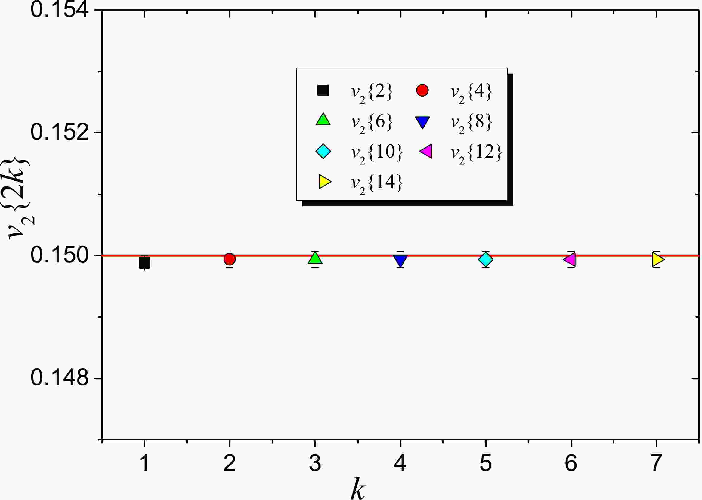
$ \sigma _{20}^2 $ and$ \sigma _{02}^2 $ , skewness$ {s_{30}} $ , and co-skewness$ {s_{12}} $ [15, 16], experimental values of at least four different cumulants v2{2}, v2{4}, v2{6}, and v2{8} are required. However, the centrality dependence of the hydrodynamic probe h = (v2{6}–v2{8})/(v2{4}– v2{6}) obtained in the experiment [16] indicates a non-zero value of the kurtosis κ40, which is the fourth central moment of the v2 distribution. Therefore, to obtain the additional fourth central moments, κ40, κ22, and κ04 [16], experimental values of at least three more cumulants of higher order, v2{10}, v2{12}, and v2{14}, are required.Therefore, to show the validity of the above method, the obtained expressions for cumulants up to the 14-th order are calculated with the azimuthal angles simulated using toy models. For each event of a given v2, a simple distribution
$p(\varphi ) = \dfrac{1}{{2\pi }} ( {1 + 2{v_2}{\rm cos}(2\varphi )} )$ is used to generate the particle azimuthal angle. We set the input value$ {v_2} = 0.15 $ with no event-by-event flow fluctuations. Thus, we expect that all v2{2k} are equal to the input value. Fig. 1 shows that this is indeed what is observed, because there is excellent agreement between the cumulant based v2{2k} estimations and the input v2 value of 0.15. Owing to a strong correlation between different$ \left\langle {\left\langle {2m} \right\rangle } \right\rangle $ [18], the statistical uncertainties on v2{2k} slowly increase with increasing k. This toy model therefore validates the method.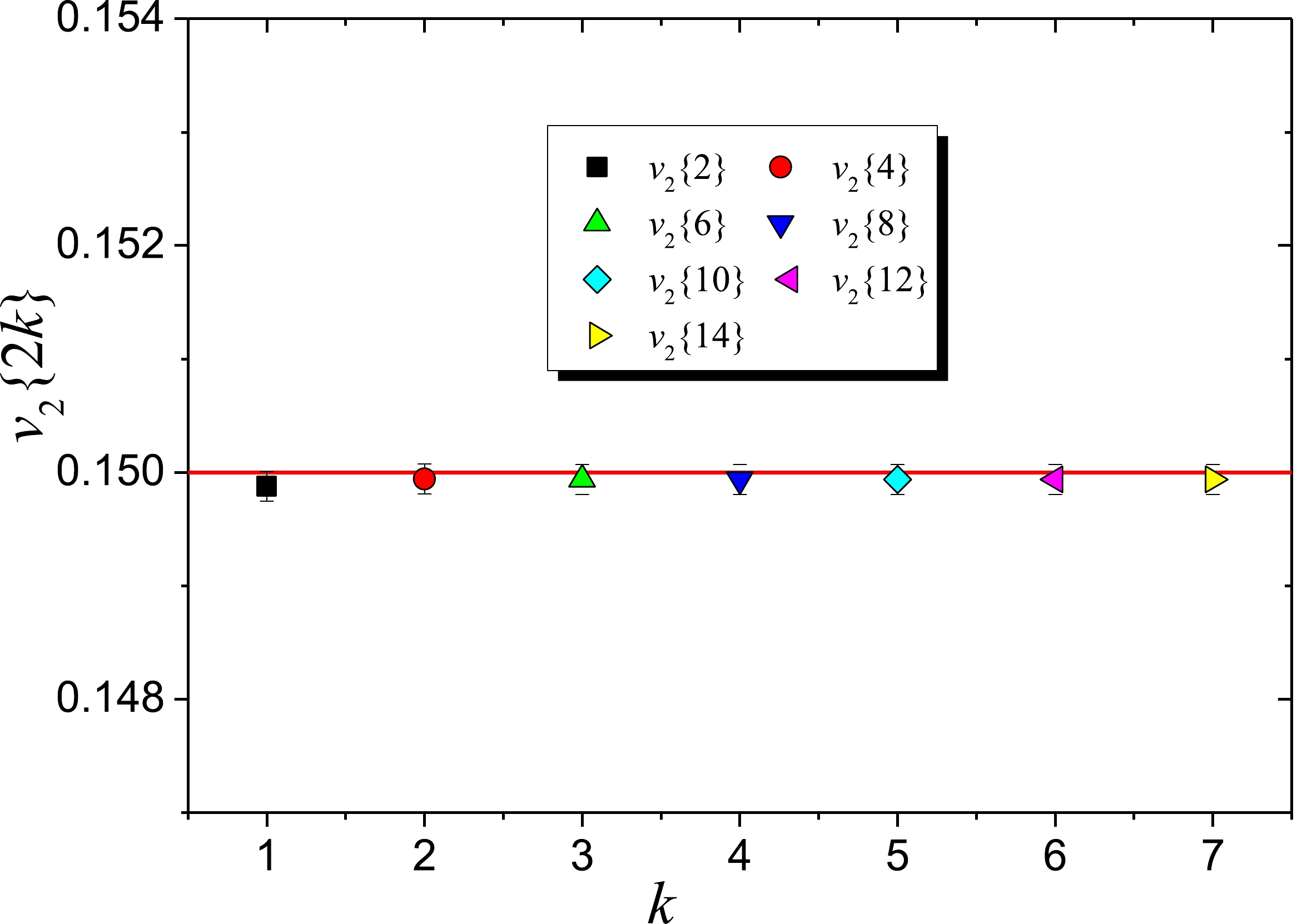
Figure 1. (color online) Cumulant based estimations of the elliptic flow v2 from toy Monte Carlo simulations. The input value of v2 is 0.15. All cumulants retrieve this input value with high precision.
However, from this validation, the sensitivity to the flow fluctuations of the higher-order cumulants cannot be verified. Therefore, we apply the second toy model, where the initial eccentricity
$ {\varepsilon _2} $ distribution is simulated using the elliptic power distribution:$ \frac{{{\rm d}N}}{{{\rm d}{\varepsilon _2}}} = \frac{{2\alpha }}{\pi }{(1 - \varepsilon _0^2)^{\alpha + 1/2}}{\varepsilon _2}{(1 - \varepsilon _2^2)^{\alpha - 1}}\int\limits_0^\pi {\frac{1}{{{{(1 - {\varepsilon _0}{\varepsilon _2}\cos \varphi )}^{2\alpha + 1}}}}{\rm d}\phi } , $

(27) where
$ \alpha $ and$ {\varepsilon _0} $ are the power and ellipticity parameters, respectively, which take different values, obtained using the Glauber model for 5.02 GeV Pb-Pb collisions, depending on the centrality [19]. The scaling factor$ {\kappa _2} $ between the elliptic flow and initial eccentricity,$ {v_2} = {\kappa _2}{\varepsilon _2} $ , is chosen to imitate the centrality dependence of the elliptic flow$ {v_2} $ measured in Ref. [16]. For each event of a given v2, a simple distribution$1 + 2{v_2}{\rm cos}(2\varphi )$ is used to generate the particle azimuthal angle. The integration in Eq. (27) can be carried out analytically to give [20]$\begin{aligned}[b] \frac{{{\rm d}N}}{{{\rm d}{\varepsilon _2}}} =& 2\alpha {(1 - \varepsilon _0^2)^{\alpha + 1/2}}{\varepsilon _2}\frac{{{{(1 - \varepsilon _2^2)}^{\alpha - 1}}}}{{{{(1 - {\varepsilon _0}{\varepsilon _2})}^{2\alpha + 1}}}}\;\\&\times{}_2{F_1}\left( {\frac{1}{2},2\alpha + 1;1;\frac{{2{\varepsilon _0}{\varepsilon _2}}}{{{\varepsilon _0}{\varepsilon _2} - 1}}} \right) .\end{aligned} $

(28) However, the ROOT version [21] of the hypergeometric function in Eq. (28) is not defined everywhere in the interval (0, 1) of
$ {\varepsilon _2} $ . Fig. 2 shows the parametric area of definition of the ROOT version of the hypergeometric function.
Figure 2. (color online) Parameter values (α, ε0) of the elliptic power distribution for 5.02 GeV Pb-Pb collisions calculated in the Glauber model for different centralities, and the area of definition of the ROOT version of the hypergeometric function
$ {}_2{F_1}\left( {\frac{1}{2},2\alpha + 1;1;\frac{{2{\varepsilon _0}{\varepsilon _2}}}{{{\varepsilon _0}{\varepsilon _2} - 1}}} \right) $ .As shown, only the centrality range 0−15% of the 5.02 GeV Pb-Pb collisions can be well simulated using this hypergeometric function. We solve this inconvenience by applying the Pfaff transformation,
$ {}_2{F_1}(a,b;c;z) = {(1 - z)^{ - b}}{}_2{F_1}\left( {c - a,b;c;\frac{z}{{z - 1}}} \right) , $

(29) which gives the following eccentricity distribution, well defined for all parameter values:
$\begin{aligned}[b] \frac{{{\rm d}N}}{{{\rm d}{\varepsilon _2}}} =& 2\alpha {(1 - \varepsilon _0^2)^{\alpha + 1/2}}{\varepsilon _2}\frac{{{{(1 - \varepsilon _2^2)}^{\alpha - 1}}}}{{{{(1 + {\varepsilon _0}{\varepsilon _2})}^{2\alpha + 1}}}}\;\\&\times{}_2{F_1}\left( {\frac{1}{2},2\alpha + 1;1;\frac{{2{\varepsilon _0}{\varepsilon _2}}}{{1 + {\varepsilon _0}{\varepsilon _2}}}} \right) .\end{aligned} $

(30) For each centrality, approximately
$ 1.5 \times 10^7 $ events are simulated using the above toy model. Figure 3 shows the$ {v_2}\{ 2k\} $ values (k = 1,…,7) calculated based on the obtained expressions for the corresponding$ \left\langle {2m} \right\rangle $ correlations as a function of centrality. A gap between$ {v_2}\{ 2\} $ and the higher-order cumulant values$ {v_2}\{ 2k\} $ (k = 2,…,7) is present. This is due to flow fluctuations, which relate the higher-order cumulants based$ {v_2}\{ 2k\} $ and the variance σv of the$ {v_2} $ distribution:$ {v_2}{\{ 2\} ^2} \approx {v_2}{\{ 2k\} ^2} + 2{\sigma ^2}_v $ for k > 1 [15]. As shown from the experimental data [16], flow fluctuations become larger moving toward peripheral collisions. The elliptic flow$ {v_2} $ values are reproduced using the expressions for$ \left\langle {2m} \right\rangle $ developed in this paper.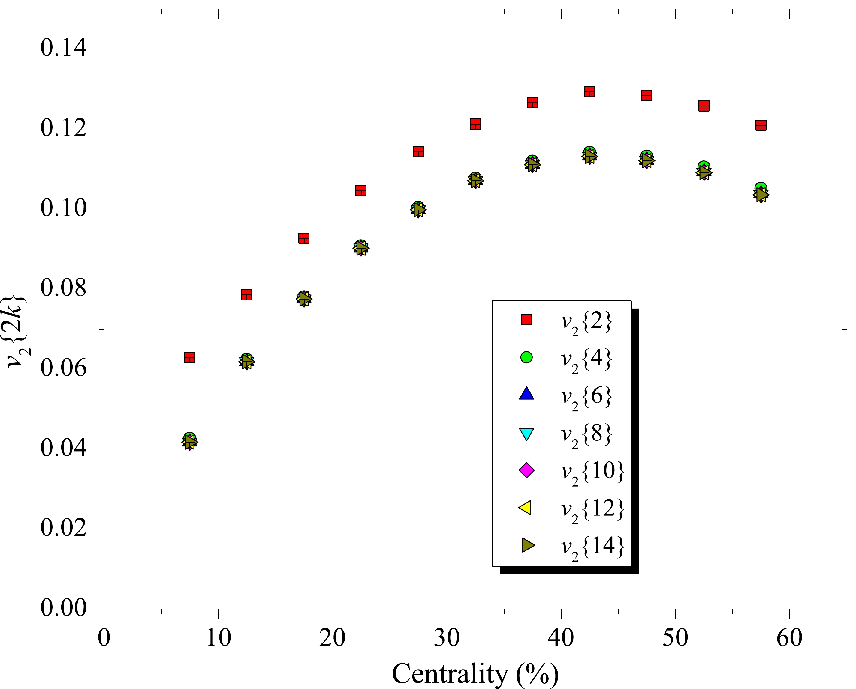
Figure 3. (color online)
$ {v_2}\{ 2k\} $ values (k = 1,…,7) as a function of centrality calculated from the data simulated using the elliptic power distribution toy model. The statistical uncertainties are negligible compared to the marker size.Because the fluctuations in the initial state are not Gaussian, the v2{2k} values for k > 1 will not be the same. This will produce a splitting between different v2{2k} values, and they will be ordered as v2{2k} > v2{2(k + 1)} for any k > 1. In Fig. 3, the ordering and fine splitting between the
$ {v_2}\{ 2k\} $ values (k = 2,…,7) are not clearly visible. To ensure that the splitting between the cumulants of different orders are explicitly visible, we show the relative differences$ ({v_2}\{ 2k\} - {v_2}\{ 14\} )/{v_2}\{ 14\} $ (k = 1,…,6) as a function of centrality in Fig. 4, where different symbols denote different cumulant orders, which are calculated from the simulated data. The corresponding input values, obtained directly by applying the elliptic power distributions, are represented by spline interpolation lines. In Fig. 4, the ordering can be clearly observed, as well as the fine splitting between cumulants of different orders. The relative difference between the cumulants decreases by approximately one order of magnitude for each increment of the order k. The excellent agreement between the lines and symbols proves the correctness of the obtained expressions for the 2m-particle azimuthal correlations$ \left\langle {2m} \right\rangle $ .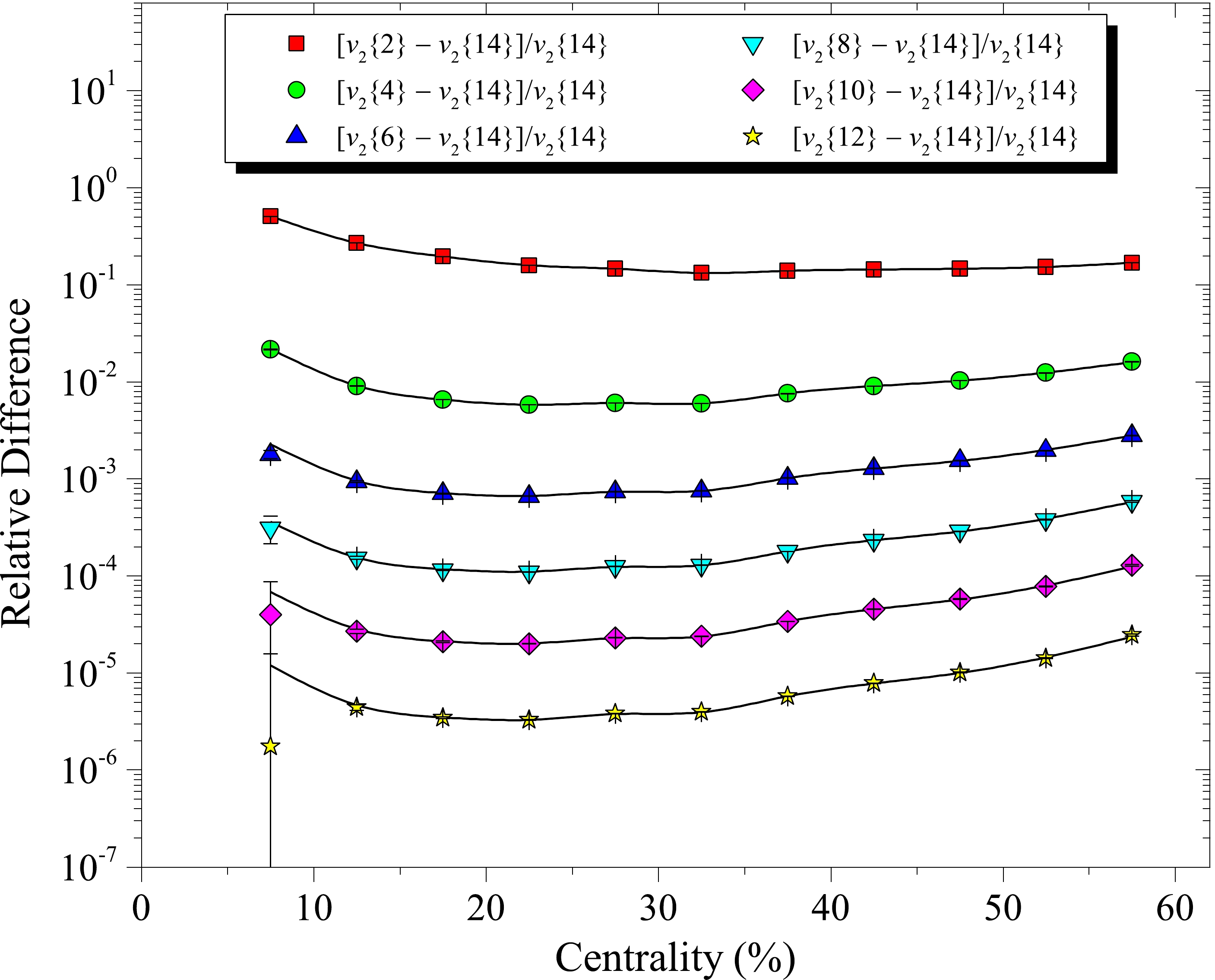
Figure 4. (color online) Relative differences
$ ({v_2}\{ 2k\} - {v_2}\{ 14\} )/ $ $ {v_2}\{ 14\} $ (k = 1,…,6) as a function of centrality. The input values, obtained directly by applying the elliptic power distributions, are represented by spline interpolation lines. -
In this paper, we present a method, based on mathematical induction, that allows us to calculate high-order
$ {v_2}\{ 2k\} $ values from Q-cumulants in a relatively straightforward way. The analytical expressions for the high 2m-particle correlations$ \left\langle {10} \right\rangle $ ,$ \left\langle {12} \right\rangle $ , and$ \left\langle {14} \right\rangle $ are obtained for the first time and given here in the form of table values. The validity of the proposed method is confirmed via an elliptic flow simulation with a toy model using the elliptic power distribution. We transform the hypergeometric function involved in the elliptic power distribution by applying Pfaff transformation and enable its calculation in the ROOT program for all parameter values of the v2 distribution. The ability to calculate high-order$ {v_2}\{ 2k\} $ values allows for the possibility of studying the fine details of the$ {v_2} $ distribution by extracting its skewness and higher central moments. Theoreticians can tune initial states in their hydrodynamic models to reconstruct the measured central moments. This can place stringent constraints on the initial geometry used in hydrodynamic calculations of the collective dynamics of QGP in high energy nuclear collisions. -
This appendix provides tables listing (Tables 5−7), for different orders of Q-cumulants, the coefficients, integer functions, and combinations of basis vectors needed to construct expressions for the 2m-particle azimuthal correlations
$ \left\langle {2m} \right\rangle $ .Table 5-continued from previous page $ i $ 

$ {x_i} $ 

$ f_i^{(m = 5,l)} $ 

Basis vectors l 42 −60 1 $ {Q_{4n}}{{ }}{Q_n}{{|}}Q_n^*Q_n^*Q_n^*Q_n^*Q_n^* $ 

5 43 600 1 $ {Q_{4n}}{{ }}{Q_n}{{|}}Q_n^*Q_n^*Q_n^*{{ }}Q_{2n}^* $ 

5 44 −900 1 $ {Q_{4n}}{{ }}{Q_n}{{|}}Q_n^*{{ }}Q_{2n}^*{{ }}Q_{2n}^* $ 

5 45 −1200 1 $ {Q_{4n}}{{ }}{Q_n}{{|}}Q_n^*Q_n^*{{ }}Q_{3n}^* $ 

5 46 1200 1 $ {Q}_{4n}{ }{Q}_{n}{|}{Q}_{2n}^{*}{ }{Q}_{3n}^{*} $ 

5 47 900 1 $ {Q_{4n}}{{ }}{Q_n}{{|}}Q_n^*{{ }}Q_{4n}^* $ 

5 48 48 1 ${Q_{5n} }{{|} }Q_n^*Q_n^*Q_n^*Q_n^*Q_n^*$ 

5 49 −480 1 ${Q_{5n} }{{|} }Q_n^*Q_n^*Q_n^*{{ } }Q_{2n}^*$ 

5 50 720 1 $ {Q_{5n}}{{ |}}Q_n^*{{ }}Q_{2n}^*{{ }}Q_{2n}^* $ 

5 51 960 1 $ {Q_{5n}}{{ |}}Q_n^*Q_n^*{{ }}Q_{3n}^* $ 

5 52 −960 1 $ {Q}_{5n}{ |}{Q}_{2n}^{*}{ }{Q}_{3n}^{*} $ 

5 53 −1440 1 $ {Q_{5n}}{{ |}}Q_n^*{{ }}Q_{4n}^* $ 

5 54 576 1 ${Q}_{5n}{|}{}{Q}_{5n}^{*}$ 

5 Table 6-continued from previous pagee $ i $ 

$ {x_i} $ 

$ f_i^{(m = 6,l)} $ 

Basis vectors l 26 16200 $ (M - 8)(M - 11) $ 

${Q}_{4n}{|}{}{Q}_{4n}^{*}$ 

4 27 −36 $ (M - 10) $ 

$ {Q_n}{Q_n}{Q_n}{Q_n}{Q_n}{{|}}Q_n^*Q_n^*Q_n^*Q_n^*Q_n^* $ 

5 28 720 $ (M - 10) $ 

$ {Q_{2n}}{{ }}{Q_n}{Q_n}{Q_n}{{|}}Q_n^*Q_n^*Q_n^*Q_n^*Q_n^* $ 

5 29 −3600 $ (M - 10) $ 

$ {Q_{2n}}{{ }}{Q_n}{Q_n}{Q_n}{{|}}Q_n^*Q_n^*Q_n^*{{ }}Q_{2n}^* $ 

5 30 −1080 $ (M - 10) $ 

$ {Q_{2n}}{{ }}{Q_{2n}}{{ }}{Q_n}{{|}}Q_n^*Q_n^*Q_n^*Q_n^*Q_n^* $ 

5 31 10800 $ (M - 10) $ 

$ {Q_{2n}}{{ }}{Q_{2n}}{{ }}{Q_n}{{|}}Q_n^*Q_n^*Q_n^*{{ }}Q_{2n}^* $ 

5 32 −8100 $ (M - 10) $ 

$ {Q_{2n}}{{ }}{Q_{2n}}{{ }}{Q_n}{{|}}Q_n^*{{ }}Q_{2n}^*{{ }}Q_{2n}^* $ 

5 33 −1440 $ (M - 10) $ 

$ {Q_{3n}}{{ }}{Q_n}{Q_n}{{|}}Q_n^*Q_n^*Q_n^*Q_n^*Q_n^* $ 

5 34 14400 $ (M - 10) $ 

$ {Q_{3n}}{{ }}{Q_n}{Q_n}{{|}}Q_n^*Q_n^*Q_n^*{{ }}Q_{2n}^* $ 

5 35 −21600 $ (M - 10) $ 

$ {Q_{3n}}{{ }}{Q_n}{Q_n}{{|}}Q_n^*{{ }}Q_{2n}^*{{ }}Q_{2n}^* $ 

5 36 −14400 $ (M - 10) $ 

$ {Q_{3n}}{{ }}{Q_n}{Q_n}{{|}}Q_n^*Q_n^*{{ }}Q_{3n}^* $ 

5 37 1440 $ (M - 10) $ 

$ {Q}_{3n}{ }{Q}_{2n}{|}{Q}_{n}^{*}{Q}_{n}^{*}{Q}_{n}^{*}{Q}_{n}^{*}{Q}_{n}^{*} $ 

5 38 −14400 $ (M - 10) $ 

$ {Q}_{3n}{ }{Q}_{2n}{|}{Q}_{n}^{*}{Q}_{n}^{*}{Q}_{n}^{*}{ }{Q}_{2n}^{*} $ 

5 39 21600 $ (M - 10) $ 

$ {Q}_{3n}{ }{Q}_{2n}{|}{Q}_{n}^{*}{ }{Q}_{2n}^{*}{ }{Q}_{2n}^{*} $ 

5 40 28800 $ (M - 10) $ 

$ {Q}_{3n}{ }{Q}_{2n}{|}{Q}_{n}^{*}{Q}_{n}^{*}{ }{Q}_{3n}^{*} $ 

5 41 −14400 $ (M - 10) $ 

$ {Q}_{3n}{ }{Q}_{2n}{|}{Q}_{2n}^{*}{ }{Q}_{3n}^{*} $ 

5 42 2160 $ (M - 10) $ 

$ {Q_{4n}}{{ }}{Q_n}{{|}}Q_n^*Q_n^*Q_n^*Q_n^*Q_n^* $ 

5 43 −21600 $ (M - 10) $ 

$ {Q_{4n}}{{ }}{Q_n}{{|}}Q_n^*Q_n^*Q_n^*{{ }}Q_{2n}^* $ 

5 44 32400 $ (M - 10) $ 

$ {Q_{4n}}{{ }}{Q_n}{{|}}Q_n^*{{ }}Q_{2n}^*{{ }}Q_{2n}^* $ 

5 45 43200 $ (M - 10) $ 

$ {Q_{4n}}{{ }}{Q_n}{{|}}Q_n^*Q_n^*{{ }}Q_{3n}^* $ 

5 46 −43200 $ (M - 10) $ 

$ {Q}_{4n}{ }{ }{Q}_{n}{|}{Q}_{2n}^{*}{ }{ }{Q}_{3n}^{*} $ 

5 47 −32400 $ (M - 10) $ 

$ {Q_{4n}}{{ }}{Q_n}{{|}}Q_n^*{{ }}Q_{4n}^* $ 

5 48 −1728 $ (M - 10) $ 

$ {Q_{5n}}{{ |}}Q_n^*Q_n^*Q_n^*Q_n^*Q_n^* $ 

5 49 17280 $ (M - 10) $ 

$ {Q_{5n}}{{ |}}Q_n^*Q_n^*Q_n^*{{ }}Q_{2n}^* $ 

5 50 −25920 $ (M - 10) $ 

$ {Q_{5n}}{{ |}}Q_n^*{{ }}Q_{2n}^*{{ }}Q_{2n}^* $ 

5 51 −34560 $ (M - 10) $ 

$ {Q_{5n}}{{ |}}Q_n^*Q_n^*{{ }}Q_{3n}^* $ 

5 52 34560 $ (M - 10) $ 

$ {Q}_{5n}{ }{|}{Q}_{2n}^{*}{ }{Q}_{3n}^{*} $ 

5 53 51840 $ (M - 10) $ 

$ {Q_{5n}}{{ |}}Q_n^*{{ }}Q_{4n}^* $ 

5 54 −20736 $ (M - 10) $ 

${Q}_{5n}{|}{}{Q}_{5n}^{*}$ 

5 55 1 1 $ {Q_n}{Q_n}{Q_n}{Q_n}{Q_n}{Q_n}{{|}}Q_n^*Q_n^*Q_n^*Q_n^*Q_n^*Q_n^* $ 

6 56 −30 1 $ {Q_{2n}}{Q_n}{Q_n}{Q_n}{Q_n}{{|}}Q_n^*Q_n^*Q_n^*Q_n^*Q_n^*Q_n^* $ 

6 57 225 1 $ {Q_{2n}}{Q_n}{Q_n}{Q_n}{Q_n}{{|}}Q_n^*Q_n^*Q_n^*Q_n^*Q_{2n}^* $ 

6 58 90 1 $ {Q_{2n}}{\kern 1pt} {Q_{2n}}{Q_n}{Q_n}{{|}}Q_n^*Q_n^*Q_n^*Q_n^*Q_n^*Q_n^* $ 

6 59 −1350 1 $ {Q_{2n}}{\kern 1pt} {Q_{2n}}{Q_n}{Q_n}{{|}}Q_n^*Q_n^*Q_n^*Q_n^*Q_{2n}^* $ 

6 60 2025 1 $ {Q_{2n}}{\kern 1pt} {Q_{2n}}{Q_n}{Q_n}{{|}}Q_n^*Q_n^*Q_{2n}^*Q_{2n}^* $ 

6 61 −30 1 ${Q_{2n} }{\kern 1pt} {Q_{2n} }{Q_{2n} }{{|} }Q_n^*Q_n^*Q_n^*Q_n^*Q_n^*Q_n^*$ 

6 62 450 1 ${Q_{2n} }{\kern 1pt} {Q_{2n} }{Q_{2n} }{{|} }Q_n^*Q_n^*Q_n^*Q_n^*Q_{2n}^*$ 

6 63 −1350 1 ${Q_{2n} }{\kern 1pt} {Q_{2n} }{Q_{2n} }{{|} }Q_n^*Q_n^*Q_{2n}^*Q_{2n}^*$ 

6 64 225 1 ${Q_{2n} }{\kern 1pt} {Q_{2n} }{Q_{2n} }{{|} }Q_{2n}^*Q_{2n}^*Q_{2n}^*$ 

6 65 80 1 $ {Q_{3n}} {Q_n}{Q_n}{Q_n}{{|}}Q_n^*Q_n^*Q_n^*Q_n^*Q_n^*Q_n^* $ 

6 66 −1200 1 $ {Q_{3n}} {Q_n}{Q_n}{Q_n}{{|}}Q_n^*Q_n^*Q_n^*Q_n^*Q_{2n}^* $ 

6 Continued on next page Table 6-continued from previous page $ i $ 

$ {x_i} $ 

$ f_i^{(m = 6,l)} $ 

Basis vectors l 67 3600 1 $ {Q_{3n}}{Q_n}{Q_n}{Q_n}{{|}}Q_n^*Q_n^*Q_{2n}^*Q_{2n}^* $ 

6 68 −1200 1 ${Q_{3n} } {Q_n}{Q_n}{Q_n}{{|} }Q_{2n}^*Q_{2n}^*Q_{2n}^*$ 

6 69 1600 1 $ {Q_{3n}} {Q_n}{Q_n}{Q_n}{{|}}Q_n^*Q_n^*Q_n^* Q_{3n}^* $ 

6 70 −240 1 $ {Q_{3n}} {Q_{2n}}{\kern 1pt} {Q_n}{{|}}Q_n^*Q_n^*Q_n^*Q_n^*Q_n^*Q_n^* $ 

6 71 3600 1 $ {Q_{3n}} {Q_{2n}}{\kern 1pt} {Q_n}{{|}}Q_n^*Q_n^*Q_n^*Q_n^*Q_{2n}^* $ 

6 72 −10800 1 $ {Q_{3n}} {Q_{2n}}{\kern 1pt} {Q_n}{{|}}Q_n^*Q_n^*Q_{2n}^*Q_{2n}^* $ 

6 73 3600 1 ${Q_{3n} } {Q_{2n} }{\kern 1pt} {Q_n}{{|} }Q_{2n}^*Q_{2n}^*Q_{2n}^*$ 

6 74 −9600 1 $ {Q_{3n}} {Q_{2n}}{\kern 1pt} {Q_n}{{|}}Q_n^*Q_n^*Q_n^* Q_{3n}^* $ 

6 75 14400 1 $ {Q_{3n}} {Q_{2n}}{\kern 1pt} {Q_n}{{|}}Q_n^*Q_{2n}^* Q_{3n}^* $ 

6 76 80 1 ${Q_{3n} } {Q_{3n} }{{|} }Q_n^*Q_n^*Q_n^*Q_n^*Q_n^*Q_n^*$ 

6 77 −1200 1 ${Q_{3n} } {Q_{3n} }{{|} }Q_n^*Q_n^*Q_n^*Q_n^*Q_{2n}^*$ 

6 78 3600 1 ${Q_{3n} } {Q_{3n} }{{|} }Q_n^*Q_n^*Q_{2n}^*Q_{2n}^*$ 

6 79 −1200 1 ${Q_{3n} } {Q_{3n} }{{|} }Q_{2n}^*Q_{2n}^*Q_{2n}^*$ 

6 80 3200 1 ${Q_{3n} } {Q_{3n} }{{|} }Q_n^*Q_n^*Q_n^* Q_{3n}^*$ 

6 81 −9600 1 ${Q_{3n} } {Q_{3n} }{{|} }Q_n^*Q_{2n}^* Q_{3n}^*$ 

6 82 1600 1 ${Q_{3n} } {Q_{3n} }{{|} }Q_{3n}^* Q_{3n}^*$ 

6 83 −180 1 $ {Q_{4n}} {Q_n}{Q_n}{{|}}Q_n^*Q_n^*Q_n^*Q_n^*Q_n^*Q_n^* $ 

6 84 2700 1 $ {Q_{4n}} {Q_n}{Q_n}{{|}}Q_n^*Q_n^*Q_n^*Q_n^*Q_{2n}^* $ 

6 85 −8100 1 $ {Q_{4n}} {Q_n}{Q_n}{{|}}Q_n^*Q_n^*Q_{2n}^*Q_{2n}^* $ 

6 86 2700 1 ${Q_{4n} } {Q_n}{Q_n}{{|} }Q_{2n}^*Q_{2n}^*Q_{2n}^*$ 

6 87 −7200 1 $ {Q_{4n}} {Q_n}{Q_n}{{|}}Q_n^*Q_n^*Q_n^* Q_{3n}^* $ 

6 88 21600 1 $ {Q_{4n}} {Q_n}{Q_n}{{|}}Q_n^*Q_{2n}^* Q_{3n}^* $ 

6 89 −7200 1 ${Q_{4n} } {Q_n}{Q_n}{{|} }Q_{3n}^* Q_{3n}^*$ 

6 90 8100 1 $ {Q_{4n}} {Q_n}{Q_n}{{|}}Q_n^*Q_n^* Q_{4n}^* $ 

6 91 180 1 ${Q_{4n} } {Q_{2n} }{{|} }Q_n^*Q_n^*Q_n^*Q_n^*Q_n^*Q_n^*$ 

6 92 −2700 1 ${Q_{4n} } {Q_{2n} }{{|} }Q_n^*Q_n^*Q_n^*Q_n^*Q_{2n}^*$ 

6 93 8100 1 ${Q_{4n} } {Q_{2n} }{{|} }Q_n^*Q_n^*Q_{2n}^*Q_{2n}^*$ 

6 94 −2700 1 ${Q_{4n} } {Q_{2n} }{{|} }Q_{2n}^*Q_{2n}^*Q_{2n}^*$ 

6 95 7200 1 ${Q_{4n} } {Q_{2n} }{{|} }Q_n^*Q_n^*Q_n^* Q_{3n}^*$ 

6 96 −21600 1 ${Q_{4n} } {Q_{2n} }{{|} }Q_n^*Q_{2n}^* Q_{3n}^*$ 

6 97 7200 1 ${Q_{4n} } {Q_{2n} }{{|} }Q_{3n}^* Q_{3n}^*$ 

6 98 −16200 1 ${Q_{4n} } {Q_{2n} }{{|} }Q_n^*Q_n^* Q_{4n}^*$ 

6 99 8100 1 ${Q_{4n} } {Q_{2n} }{{|} }Q_{2n}^* Q_{4n}^*$ 

6 100 288 1 $ {Q_{5n}} {Q_n}{{|}}Q_n^*Q_n^*Q_n^*Q_n^*Q_n^*Q_n^* $ 

6 101 −4320 1 $ {Q_{5n}} {Q_n}{{|}}Q_n^*Q_n^*Q_n^*Q_n^*Q_{2n}^* $ 

6 102 12960 1 $ {Q_{5n}} {Q_n}{{|}}Q_n^*Q_n^*Q_{2n}^*Q_{2n}^* $ 

6 103 −4320 1 ${Q_{5n} } {Q_n}{{|} }Q_{2n}^*Q_{2n}^*Q_{2n}^*$ 

6 104 11520 1 $ {Q_{5n}} {Q_n}{{|}}Q_n^*Q_n^*Q_n^* Q_{3n}^* $ 

6 105 −34560 1 $ {Q_{5n}} {Q_n}{{|}}Q_n^*Q_{2n}^* Q_{3n}^* $ 

6 106 11520 1 ${Q_{5n} } {Q_n}{{|} }Q_{3n}^* Q_{3n}^*$ 

6 107 −25920 1 $ {Q_{5n}} {Q_n}{{|}}Q_n^*Q_n^* Q_{4n}^* $ 

6 Continued on next page Table 6-continued from previous page $ i $ 

$ {x_i} $ 

$ f_i^{(m = 6,l)} $ 

Basis vectors l 108 25920 1 ${Q_{5n} } {Q_n}{{|} }Q_{2n}^* Q_{4n}^*$ 

6 109 20736 1 $ {Q_{5n}} {Q_n}{{|}}Q_n^* Q_{5n}^* $ 

6 110 -240 1 $ {Q_{6n}} {{|}}Q_n^*Q_n^*Q_n^*Q_n^*Q_n^*Q_n^* $ 

6 111 3600 1 $ {Q_{6n}} {{|}}Q_n^*Q_n^*Q_n^*Q_n^*Q_{2n}^* $ 

6 112 −10800 1 $ {Q_{6n}} {{|}}Q_n^*Q_n^*Q_{2n}^*Q_{2n}^* $ 

6 113 3600 1 ${Q_{6n} } {{|} }Q_{2n}^*Q_{2n}^*Q_{2n}^*$ 

6 114 −9600 1 $ {Q_{6n}} {{|}}Q_n^*Q_n^*Q_n^* Q_{3n}^* $ 

6 115 28800 1 $ {Q_{6n}} {{|}}Q_n^*Q_{2n}^* Q_{3n}^* $ 

6 116 −9600 1 ${Q_{6n} } {{|} }Q_{3n}^* Q_{3n}^*$ 

6 117 21600 1 $ {Q_{6n}} {{|}}Q_n^*Q_n^* Q_{4n}^* $ 

6 118 −21600 1 ${Q_{6n} } {{|} }Q_{2n}^* Q_{4n}^*$ 

6 119 −34560 1 $ {Q_{6n}} {{|}}Q_n^* Q_{5n}^* $ 

6 120 14400 1 ${Q_{6n} } {{|} } Q_{6n}^*$ 

6 $ i $ 

$ {x_i} $ 

$ f_i^{(m = 7,l)} $ 

Basis vectors l 1 −5040 $ M(M - 8)(M - 9)(M - 10)(M - 11)(M - 12)(M - 13) $ 

$ 1 $ 

0 2 35280 $ (M - 2)(M - 9)(M - 10)(M - 11)(M - 12)(M - 13) $ 

$ {Q_n}|Q_n^* $ 

1 3 −52920 $ (M - 4)(M - 10)(M - 11)(M - 12)(M - 13) $ 

$ {Q_n}{Q_n}|Q_n^*Q_n^* $ 

2 4 105840 $ (M - 4)(M - 10)(M - 11)(M - 12)(M - 13) $ 

$ {Q_{2n}}{{ }}|Q_n^*Q_n^* $ 

2 5 −52920 $ (M - 4)(M - 10)(M - 11)(M - 12)(M - 13) $ 

$ {Q_{2n}}{{ }}|{{ }}Q_{2n}^* $ 

2 6 29400 $ (M - 6)(M - 11)(M - 12)(M - 13) $ 

$ {Q}_{n}{Q}_{n}{Q}_{n}�{|}{Q}_{n}^{*}{Q}_{n}^{*}{Q}_{n}^{*} $ 

3 7 −176400 $ (M - 6)(M - 11)(M - 12)(M - 13) $ 

$ {Q_{2n}}{{ }}{Q_n}{{|}}Q_n^*Q_n^*Q_n^* $ 

3 8 264600 $ (M - 6)(M - 11)(M - 12)(M - 13) $ 

$ {Q_{2n}}{{ }}{Q_n}{{|}}Q_n^*{{ }}Q_{2n}^* $ 

3 9 117600 $ (M - 6)(M - 11)(M - 12)(M - 13) $ 

$ {Q_{3n}}{{ |}}Q_n^*Q_n^*Q_n^* $ 

3 10 −352800 $ (M - 6)(M - 11)(M - 12)(M - 13) $ 

$ {Q_{3n}}{{ |}}Q_n^*{{ }}Q_{2n}^* $ 

3 11 117600 $ (M - 6)(M - 11)(M - 12)(M - 13) $ 

${Q}_{3n}{|}{}{Q}_{3n}^{*}$ 

3 12 −7350 $ (M - 8)(M - 12)(M - 13) $ 

$ {Q_n}{Q_n}{Q_n}{Q_n}{{|}}Q_n^*Q_n^*Q_n^*Q_n^* $ 

4 13 88200 $ (M - 8)(M - 12)(M - 13) $ 

$ {Q_{2n}}{{ }}{Q_n}{Q_n}{{|}}Q_n^*Q_n^*Q_n^*Q_n^* $ 

4 14 −264600 $ (M - 8)(M - 12)(M - 13) $ 

$ {Q_{2n}}{{ }}{Q_n}{Q_n}{{|}}Q_n^*Q_n^*{{ }}Q_{2n}^* $ 

4 15 −44100 $ (M - 8)(M - 12)(M - 13) $ 

$ {Q_{2n}}{{ }}{Q_{2n}}{{ |}}Q_n^*Q_n^*Q_n^*Q_n^* $ 

4 16 264600 $ (M - 8)(M - 12)(M - 13) $ 

$ {Q_{2n}}{{ }}{Q_{2n}}{{ |}}Q_n^*Q_n^*{{ }}Q_{2n}^* $ 

4 17 −66150 $ (M - 8)(M - 12)(M - 13) $ 

$ {Q_{2n}}{{ }}{Q_{2n}}{{ | }}Q_{2n}^*{{ }}Q_{2n}^* $ 

4 18 −117600 $ (M - 8)(M - 12)(M - 13) $ 

$ {Q_{3n}}{{ }}{Q_n}{{|}}Q_n^*Q_n^*Q_n^*Q_n^* $ 

4 19 705600 $ (M - 8)(M - 12)(M - 13) $ 

$ {Q_{3n}}{{ }}{Q_n}{{|}}Q_n^*Q_n^*{{ }}Q_{2n}^* $ 

4 20 −352800 $ (M - 8)(M - 12)(M - 13) $ 

$ {Q_{3n}}{{ }}{Q_n}{{| }}Q_{2n}^*{{ }}Q_{2n}^* $ 

4 21 −470400 $ (M - 8)(M - 12)(M - 13) $ 

$ {Q_{3n}}{{ }}{Q_n}{{|}}Q_n^*{{ }}Q_{3n}^* $ 

4 22 88200 $ (M - 8)(M - 12)(M - 13) $ 

$ {Q_{4n}}{{ |}}Q_n^*Q_n^*Q_n^*Q_n^* $ 

4 23 −529200 $ (M - 8)(M - 12)(M - 13) $ 

$ {Q_{4n}}{{ |}}Q_n^*Q_n^*{{ }}Q_{2n}^* $ 

4 24 264600 $ (M - 8)(M - 12)(M - 13) $ 

$ {Q_{4n}}{{ | }}Q_{2n}^*{{ }}Q_{2n}^* $ 

4 25 705600 $ (M - 8)(M - 12)(M - 13) $ 

$ {Q_{4n}}{{ |}}Q_n^*{{ }}Q_{3n}^* $ 

4 Continued on next page Table 7. Coefficients, integer functions, and basis vectors for the calculation of the fourteen-particle azimuthal correlations.
Table 7-continued from previous page $ i $ 

$ {x_i} $ 

$ f_i^{(m = 7,l)} $ 

Basis vectors l 26 −264600 $ (M - 8)(M - 12)(M - 13) $ 

$ {Q}_{4n}{ |}{ }{Q}_{4n}^{*} $ 

4 27 882 $ (M - 10)(M - 13) $ 

$ {Q_n}{Q_n}{Q_n}{Q_n}{Q_n}{{|}}Q_n^*Q_n^*Q_n^*Q_n^*Q_n^* $ 

5 28 −17640 $ (M - 10)(M - 13) $ 

$ {Q_{2n}}{{ }}{Q_n}{Q_n}{Q_n}{{|}}Q_n^*Q_n^*Q_n^*Q_n^*Q_n^* $ 

5 29 88200 $ (M - 10)(M - 13) $ 

$ {Q_{2n}}{{ }}{Q_n}{Q_n}{Q_n}{{|}}Q_n^*Q_n^*Q_n^*{{ }}Q_{2n}^* $ 

5 30 26460 $ (M - 10)(M - 13) $ 

$ {Q_{2n}}{{ }}{Q_{2n}}{{ }}{Q_n}{{|}}Q_n^*Q_n^*Q_n^*Q_n^*Q_n^* $ 

5 31 −264600 $ (M - 10)(M - 13) $ 

$ {Q_{2n}}{{ }}{Q_{2n}}{{ }}{Q_n}{{|}}Q_n^*Q_n^*Q_n^*{{ }}Q_{2n}^* $ 

5 32 198450 $ (M - 10)(M - 13) $ 

$ {Q_{2n}}{{ }}{Q_{2n}}{{ }}{Q_n}{{|}}Q_n^*{{ }}Q_{2n}^*{{ }}Q_{2n}^* $ 

5 33 35280 $ (M - 10)(M - 13) $ 

$ {Q_{3n}}{{ }}{Q_n}{Q_n}{{|}}Q_n^*Q_n^*Q_n^*Q_n^*Q_n^* $ 

5 34 −352800 $ (M - 10)(M - 13) $ 

$ {Q_{3n}}{{ }}{Q_n}{Q_n}{{|}}Q_n^*Q_n^*Q_n^*{{ }}Q_{2n}^* $ 

5 35 529200 $ (M - 10)(M - 13) $ 

$ {Q_{3n}}{{ }}{Q_n}{Q_n}{{|}}Q_n^*{{ }}Q_{2n}^*{{ }}Q_{2n}^* $ 

5 36 352800 $ (M - 10)(M - 13) $ 

$ {Q_{3n}}{{ }}{Q_n}{Q_n}{{|}}Q_n^*Q_n^*{{ }}Q_{3n}^* $ 

5 37 −35280 $ (M - 10)(M - 13) $ 

$ {Q}_{3n}{ }{Q}_{2n}{|}{Q}_{n}^{*}{Q}_{n}^{*}{Q}_{n}^{*}{Q}_{n}^{*}{Q}_{n}^{*} $ 

5 38 352800 $ (M - 10)(M - 13) $ 

$ {Q}_{3n}{ }{Q}_{2n}{|}{Q}_{n}^{*}{Q}_{n}^{*}{Q}_{n}^{*}{ }{Q}_{2n}^{*} $ 

5 39 −529200 $ (M - 10)(M - 13) $ 

$ {Q}_{3n}{ }{Q}_{2n}{|}{Q}_{n}^{*}{ }{Q}_{2n}^{*}{ }{Q}_{2n}^{*} $ 

5 40 −705600 $ (M - 10)(M - 13) $ 

$ {Q}_{3n}{ }{Q}_{2n}{|}{Q}_{n}^{*}{Q}_{n}^{*}{ }{Q}_{3n}^{*} $ 

5 41 352800 $ (M - 10)(M - 13) $ 

$ {Q}_{3n}{ }{Q}_{2n}{|}{Q}_{2n}^{*}{ }{Q}_{3n}^{*} $ 

5 42 −52920 $ (M - 10)(M - 13) $ 

$ {Q_{4n}}{{ }}{Q_n}{{|}}Q_n^*Q_n^*Q_n^*Q_n^*Q_n^* $ 

5 43 529200 $ (M - 10)(M - 13) $ 

$ {Q_{4n}}{{ }}{Q_n}{{|}}Q_n^*Q_n^*Q_n^*{{ }}Q_{2n}^* $ 

5 44 −793800 $ (M - 10)(M - 13) $ 

$ {Q_{4n}}{{ }}{Q_n}{{|}}Q_n^*{{ }}Q_{2n}^*{{ }}Q_{2n}^* $ 

5 45 −1058400 $ (M - 10)(M - 13) $ 

$ {Q_{4n}}{{ }}{Q_n}{{|}}Q_n^*Q_n^*{{ }}Q_{3n}^* $ 

5 46 1058400 $ (M - 10)(M - 13) $ 

$ {Q}_{4n}{ }{ }{Q}_{n}{|}{Q}_{2n}^{*}{ }{ }{Q}_{3n}^{*} $ 

5 47 793800 $ (M - 10)(M - 13) $ 

$ {Q_{4n}}{{ }}{Q_n}{{|}}Q_n^*{{ }}Q_{4n}^* $ 

5 48 42336 $ (M - 10)(M - 13) $ 

$ {Q_{5n}}{{ |}}Q_n^*Q_n^*Q_n^*Q_n^*Q_n^* $ 

5 49 −423360 $ (M - 10)(M - 13) $ 

$ {Q_{5n}}{{ |}}Q_n^*Q_n^*Q_n^*{{ }}Q_{2n}^* $ 

5 50 635040 $ (M - 10)(M - 13) $ 

$ {Q_{5n}}{{ |}}Q_n^*{{ }}Q_{2n}^*{{ }}Q_{2n}^* $ 

5 51 846720 $ (M - 10)(M - 13) $ 

$ {Q_{5n}}{{ |}}Q_n^*Q_n^*{{ }}Q_{3n}^* $ 

5 52 −846720 $ (M - 10)(M - 13) $ 

$ {Q}_{5n}{ }{|}{Q}_{2n}^{*}{ }{Q}_{3n}^{*} $ 

5 53 −1270080 $ (M - 10)(M - 13) $ 

$ {Q_{5n}}{{ |}}Q_n^*{{ }}Q_{4n}^* $ 

5 54 508032 $ (M - 10)(M - 13) $ 

$ {Q}_{5n}{ |}{ }{Q}_{5n}^{*} $ 

5 55 −49 $ (M - 12) $ 

$ {Q_n}{Q_n}{Q_n}{Q_n}{Q_n}{Q_n}{{|}}Q_n^*Q_n^*Q_n^*Q_n^*Q_n^*Q_n^* $ 

6 56 1470 $ (M - 12) $ 

$ {Q_{2n}}{Q_n}{Q_n}{Q_n}{Q_n}{{|}}Q_n^*Q_n^*Q_n^*Q_n^*Q_n^*Q_n^* $ 

6 57 −11025 $ (M - 12) $ 

$ {Q_{2n}}{Q_n}{Q_n}{Q_n}{Q_n}{{|}}Q_n^*Q_n^*Q_n^*Q_n^*Q_{2n}^* $ 

6 58 −4410 $ (M - 12) $ 

$ {Q_{2n}}{\kern 1pt} {Q_{2n}}{Q_n}{Q_n}{{|}}Q_n^*Q_n^*Q_n^*Q_n^*Q_n^*Q_n^* $ 

6 59 66150 $ (M - 12) $ 

$ {Q_{2n}}{\kern 1pt} {Q_{2n}}{Q_n}{Q_n}{{|}}Q_n^*Q_n^*Q_n^*Q_n^*Q_{2n}^* $ 

6 60 −99225 $ (M - 12) $ 

$ {Q_{2n}}{\kern 1pt} {Q_{2n}}{Q_n}{Q_n}{{|}}Q_n^*Q_n^*Q_{2n}^*Q_{2n}^* $ 

6 61 1470 $ (M - 12) $ 

${Q_{2n} }{\kern 1pt} {Q_{2n} }{Q_{2n} }{{|} }Q_n^*Q_n^*Q_n^*Q_n^*Q_n^*Q_n^*$ 

6 62 −22050 $ (M - 12) $ 

${Q_{2n} }{\kern 1pt} {Q_{2n} }{Q_{2n} }{{|} }Q_n^*Q_n^*Q_n^*Q_n^*Q_{2n}^*$ 

6 63 66150 $ (M - 12) $ 

${Q_{2n} }{\kern 1pt} {Q_{2n} }{Q_{2n} }{{|} }Q_n^*Q_n^*Q_{2n}^*Q_{2n}^*$ 

6 64 −11025 $ (M - 12) $ 

${Q_{2n} }{\kern 1pt} {Q_{2n} }{Q_{2n} }{{|} }Q_{2n}^*Q_{2n}^*Q_{2n}^*$ 

6 65 −3920 $ (M - 12) $ 

$ {Q_{3n}}{Q_n}{Q_n}{Q_n}{{|}}Q_n^*Q_n^*Q_n^*Q_n^*Q_n^*Q_n^* $ 

6 66 58800 $ (M - 12) $ 

$ {Q_{3n}} {Q_n}{Q_n}{Q_n}{{|}}Q_n^*Q_n^*Q_n^*Q_n^*Q_{2n}^* $ 

6 Continued on next page Table 7-continued from previous page $ i $ 

$ {x_i} $ 

$ f_i^{(m = 7,l)} $ 

Basis vectors l 67 −176400 $ (M - 12) $ 

$ {Q_{3n}} {Q_n}{Q_n}{Q_n}{{|}}Q_n^*Q_n^*Q_{2n}^*Q_{2n}^* $ 

6 68 58800 $ (M - 12) $ 

${Q_{3n} } {Q_n}{Q_n}{Q_n}{{|} }Q_{2n}^*Q_{2n}^*Q_{2n}^*$ 

6 69 −78400 $ (M - 12) $ 

$ {Q_{3n}}{Q_n}{Q_n}{Q_n}{{|}}Q_n^*Q_n^*Q_n^*Q_{3n}^* $ 

6 70 11760 $ (M - 12) $ 

$ {Q_{3n}} {Q_{2n}}{\kern 1pt} {Q_n}{{|}}Q_n^*Q_n^*Q_n^*Q_n^*Q_n^*Q_n^* $ 

6 71 −176400 $ (M - 12) $ 

$ {Q_{3n}} {Q_{2n}}{\kern 1pt} {Q_n}{{|}}Q_n^*Q_n^*Q_n^*Q_n^*Q_{2n}^* $ 

6 72 529200 $ (M - 12) $ 

$ {Q_{3n}} {Q_{2n}}{\kern 1pt} {Q_n}{{|}}Q_n^*Q_n^*Q_{2n}^*Q_{2n}^* $ 

6 73 −176400 $ (M - 12) $ 

${Q_{3n} } {Q_{2n} }{\kern 1pt} {Q_n}{{|} }Q_{2n}^*Q_{2n}^*Q_{2n}^*$ 

6 74 470400 $ (M - 12) $ 

$ {Q_{3n}} {Q_{2n}}{\kern 1pt} {Q_n}{{|}}Q_n^*Q_n^*Q_n^* Q_{3n}^* $ 

6 75 −705600 $ (M - 12) $ 

$ {Q_{3n}} {Q_{2n}}{\kern 1pt} {Q_n}{{|}}Q_n^*Q_{2n}^* Q_{3n}^* $ 

6 76 −3920 $ (M - 12) $ 

${Q_{3n} } {Q_{3n} }{{|} }Q_n^*Q_n^*Q_n^*Q_n^*Q_n^*Q_n^*$ 

6 77 58800 $ (M - 12) $ 

${Q_{3n} } {Q_{3n} }{{|} }Q_n^*Q_n^*Q_n^*Q_n^*Q_{2n}^*$ 

6 78 −176400 $ (M - 12) $ 

${Q_{3n} } {Q_{3n} }{{|} }Q_n^*Q_n^*Q_{2n}^*Q_{2n}^*$ 

6 79 58800 $ (M - 12) $ 

${Q_{3n} } {Q_{3n} }{{|} }Q_{2n}^*Q_{2n}^*Q_{2n}^*$ 

6 80 −156800 $ (M - 12) $ 

${Q_{3n} } {Q_{3n} }{{|} }Q_n^*Q_n^*Q_n^* Q_{3n}^*$ 

6 81 470400 $ (M - 12) $ 

${Q_{3n} } {Q_{3n} }{{|} }Q_n^*Q_{2n}^* Q_{3n}^*$ 

6 82 −78400 $ (M - 12) $ 

${Q_{3n} } {Q_{3n} }{{|} }Q_{3n}^* Q_{3n}^*$ 

6 83 8820 $ (M - 12) $ 

$ {Q_{4n}} {Q_n}{Q_n}{{|}}Q_n^*Q_n^*Q_n^*Q_n^*Q_n^*Q_n^* $ 

6 84 −132300 $ (M - 12) $ 

$ {Q_{4n}} {Q_n}{Q_n}{{|}}Q_n^*Q_n^*Q_n^*Q_n^*Q_{2n}^* $ 

6 85 396900 $ (M - 12) $ 

$ {Q_{4n}} {Q_n}{Q_n}{{|}}Q_n^*Q_n^*Q_{2n}^*Q_{2n}^* $ 

6 86 −132300 $ (M - 12) $ 

${Q_{4n} } {Q_n}{Q_n}{{|} }Q_{2n}^*Q_{2n}^*Q_{2n}^*$ 

6 87 352800 $ (M - 12) $ 

$ {Q_{4n}} {Q_n}{Q_n}{{|}}Q_n^*Q_n^*Q_n^* Q_{3n}^* $ 

6 88 −1058400 $ (M - 12) $ 

$ {Q_{4n}} {Q_n}{Q_n}{{|}}Q_n^*Q_{2n}^* Q_{3n}^* $ 

6 89 352800 $ (M - 12) $ 

${Q_{4n} } {Q_n}{Q_n}{{|} }Q_{3n}^* Q_{3n}^*$ 

6 90 −396900 $ (M - 12) $ 

$ {Q_{4n}} {Q_n}{Q_n}{{|}}Q_n^*Q_n^* Q_{4n}^* $ 

6 91 −8820 $ (M - 12) $ 

${Q_{4n} } {Q_{2n} }{{|} }Q_n^*Q_n^*Q_n^*Q_n^*Q_n^*Q_n^*$ 

6 92 132300 $ (M - 12) $ 

${Q_{4n} } {Q_{2n} }{{|} }Q_n^*Q_n^*Q_n^*Q_n^*Q_{2n}^*$ 

6 93 −396900 $ (M - 12) $ 

${Q_{4n} } {Q_{2n} }{{|} }Q_n^*Q_n^*Q_{2n}^*Q_{2n}^*$ 

6 94 132300 $ (M - 12) $ 

${Q_{4n} } {Q_{2n} }{{|} }Q_{2n}^*Q_{2n}^*Q_{2n}^*$ 

6 95 −352800 $ (M - 12) $ 

${Q_{4n} } {Q_{2n} }{{|} }Q_n^*Q_n^*Q_n^* Q_{3n}^*$ 

6 96 1058400 $ (M - 12) $ 

${Q_{4n} } {Q_{2n} }{{|} }Q_n^*Q_{2n}^* Q_{3n}^*$ 

6 97 −352800 $ (M - 12) $ 

${Q_{4n} } {Q_{2n} }{{|} }Q_{3n}^* Q_{3n}^*$ 

6 98 793800 $ (M - 12) $ 

${Q_{4n} } {Q_{2n} }{{|} }Q_n^*Q_n^* Q_{4n}^*$ 

6 99 −396900 $ (M - 12) $ 

${Q_{4n} } {Q_{2n} }{{|} }Q_{2n}^* Q_{4n}^*$ 

6 100 −14112 $ (M - 12) $ 

$ {Q_{5n}} {Q_n}{{|}}Q_n^*Q_n^*Q_n^*Q_n^*Q_n^*Q_n^* $ 

6 101 211680 $ (M - 12) $ 

$ {Q_{5n}} {Q_n}{{|}}Q_n^*Q_n^*Q_n^*Q_n^*Q_{2n}^* $ 

6 102 −635040 $ (M - 12) $ 

$ {Q_{5n}} {Q_n}{{|}}Q_n^*Q_n^*Q_{2n}^*Q_{2n}^* $ 

6 103 211680 $ (M - 12) $ 

${Q_{5n} } {Q_n}{{|} }Q_{2n}^*Q_{2n}^*Q_{2n}^*$ 

6 104 −564480 $ (M - 12) $ 

$ {Q_{5n}} {Q_n}{{|}}Q_n^*Q_n^*Q_n^* Q_{3n}^* $ 

6 105 1693440 $ (M - 12) $ 

$ {Q_{5n}} {Q_n}{{|}}Q_n^*Q_{2n}^* Q_{3n}^* $ 

6 106 −564480 $ (M - 12) $ 

${Q_{5n} } {Q_n}{{|} }Q_{3n}^* Q_{3n}^*$ 

6 107 1270080 $ (M - 12) $ 

$ {Q_{5n}} {Q_n}{{|}}Q_n^*Q_n^* Q_{4n}^* $ 

6 Continued on next page Table 7-continued from previous page $ i $ 

$ {x_i} $ 

$ f_i^{(m = 7,l)} $ 

Basis vectors l 108 −1270080 $ (M - 12) $ 

${Q_{5n} }{Q_n}{{|} }Q_{2n}^*Q_{4n}^*$ 

6 109 −1016064 $ (M - 12) $ 

$ {Q_{5n}} {Q_n}{{|}}Q_n^* Q_{5n}^* $ 

6 110 11760 $ (M - 12) $ 

$ {Q_{6n}} {{|}}Q_n^*Q_n^*Q_n^*Q_n^*Q_n^*Q_n^* $ 

6 111 −176400 $ (M - 12) $ 

$ {Q_{6n}} {{|}}Q_n^*Q_n^*Q_n^*Q_n^*Q_{2n}^* $ 

6 112 529200 $ (M - 12) $ 

$ {Q_{6n}} {{|}}Q_n^*Q_n^*Q_{2n}^*Q_{2n}^* $ 

6 113 −176400 $ (M - 12) $ 

${Q_{6n} } {{|} }Q_{2n}^*Q_{2n}^*Q_{2n}^*$ 

6 114 470400 $ (M - 12) $ 

$ {Q_{6n}} {{|}}Q_n^*Q_n^*Q_n^* Q_{3n}^* $ 

6 115 −1411200 $ (M - 12) $ 

$ {Q_{6n}} {{|}}Q_n^*Q_{2n}^* Q_{3n}^* $ 

6 116 470400 $ (M - 12) $ 

${Q_{6n} } {{|} }Q_{3n}^* Q_{3n}^*$ 

6 117 −1058400 $ (M - 12) $ 

$ {Q_{6n}} {{|}}Q_n^*Q_n^* Q_{4n}^* $ 

6 118 1058400 $ (M - 12) $ 

${Q_{6n} } {{|} }Q_{2n}^* Q_{4n}^*$ 

6 119 1693440 $ (M - 12) $ 

$ {Q_{6n}} {{|}}Q_n^* Q_{5n}^* $ 

6 120 −705600 $ (M - 12) $ 

${Q_{6n} } {{|} } Q_{6n}^*$ 

6 121 1 1 $ {Q_n}{Q_n}{Q_n}{Q_n}{Q_n}{Q_n}{Q_n}|Q_n^*Q_n^*Q_n^*Q_n^*Q_n^*Q_n^*Q_n^* $ 

7 122 −42 1 $ {Q_{2n}}{Q_n}{Q_n}{Q_n}{Q_n}{Q_n}|Q_n^*Q_n^*Q_n^*Q_n^*Q_n^*Q_n^*Q_n^* $ 

7 123 441 1 $ {Q_{2n}}{Q_n}{Q_n}{Q_n}{Q_n}{Q_n}|Q_n^*Q_n^*Q_n^*Q_n^*Q_n^*Q_{2n}^* $ 

7 124 210 1 $ {Q_{2n}}{Q_{2n}}{Q_n}{Q_n}{Q_n}|Q_n^*Q_n^*Q_n^*Q_n^*Q_n^*Q_n^*Q_n^* $ 

7 125 −4410 1 $ {Q_{2n}}{Q_{2n}}{Q_n}{Q_n}{Q_n}|Q_n^*Q_n^*Q_n^*Q_n^*Q_n^*Q_{2n}^* $ 

7 126 11025 1 $ {Q_{2n}}{Q_{2n}}{Q_n}{Q_n}{Q_n}|Q_n^*Q_n^*Q_n^*Q_{2n}^*Q_{2n}^* $ 

7 127 −210 1 $ {Q_{2n}}{Q_{2n}}{Q_{2n}}{Q_n}|Q_n^*Q_n^*Q_n^*Q_n^*Q_n^*Q_n^*Q_n^* $ 

7 128 4410 1 $ {Q_{2n}}{Q_{2n}}{Q_{2n}}{Q_n}|Q_n^*Q_n^*Q_n^*Q_n^*Q_n^*Q_{2n}^* $ 

7 129 −22050 1 $ {Q_{2n}}{Q_{2n}}{Q_{2n}}{Q_n}|Q_n^*Q_n^*Q_n^*Q_{2n}^*Q_{2n}^* $ 

7 130 11025 1 $ {Q_{2n}}{Q_{2n}}{Q_{2n}}{Q_n}|Q_n^*Q_{2n}^*Q_{2n}^*Q_{2n}^* $ 

7 131 140 1 $ {Q_{3n}}{Q_n}{Q_n}{Q_n}{Q_n}|Q_n^*Q_n^*Q_n^*Q_n^*Q_n^*Q_n^*Q_n^* $ 

7 132 −2940 1 $ {Q_{3n}}{Q_n}{Q_n}{Q_n}{Q_n}|Q_n^*Q_n^*Q_n^*Q_n^*Q_n^*Q_{2n}^* $ 

7 133 14700 1 $ {Q_{3n}}{Q_n}{Q_n}{Q_n}{Q_n}|Q_n^*Q_n^*Q_n^*Q_{2n}^*Q_{2n}^* $ 

7 134 −14700 1 $ {Q_{3n}}{Q_n}{Q_n}{Q_n}{Q_n}|Q_n^*Q_{2n}^*Q_{2n}^*Q_{2n}^* $ 

7 135 4900 1 $ {Q_{3n}} {Q_n}{Q_n}{Q_n}{Q_n}|Q_n^*Q_n^*Q_n^*Q_n^* Q_{3n}^* $ 

7 136 −840 1 $ {Q_{3n}}{Q_{2n}}{Q_n}{Q_n}|Q_n^*Q_n^*Q_n^*Q_n^*Q_n^*Q_n^*Q_n^* $ 

7 137 17640 1 $ {Q_{3n}}{Q_{2n}}{Q_n}{Q_n}|Q_n^*Q_n^*Q_n^*Q_n^*Q_n^*Q_{2n}^* $ 

7 138 −88200 1 $ {Q_{3n}}{Q_{2n}}{Q_n}{Q_n}|Q_n^*Q_n^*Q_n^*Q_{2n}^*Q_{2n}^* $ 

7 139 88200 1 $ {Q_{3n}}{Q_{2n}}{Q_n}{Q_n}|Q_n^*Q_{2n}^*Q_{2n}^*Q_{2n}^* $ 

7 140 −58800 1 $ {Q_{3n}}{Q_{2n}}{Q_n}{Q_n}|Q_n^*Q_n^*Q_n^*Q_n^*Q_{3n}^* $ 

7 141 176400 1 $ {Q_{3n}}{Q_{2n}}{Q_n}{Q_n}|Q_n^*Q_n^*Q_{2n}^*Q_{3n}^* $ 

7 142 420 1 $ {Q_{3n}}{Q_{2n}}{Q_{2n}}|Q_n^*Q_n^*Q_n^*Q_n^*Q_n^*Q_n^*Q_n^* $ 

7 143 −8820 1 $ {Q_{3n}}{Q_{2n}}{Q_{2n}}|Q_n^*Q_n^*Q_n^*Q_n^*Q_n^*Q_{2n}^* $ 

7 144 44100 1 $ {Q_{3n}}{Q_{2n}}{Q_{2n}}|Q_n^*Q_n^*Q_n^*Q_{2n}^*Q_{2n}^* $ 

7 145 −44100 1 $ {Q_{3n}}{Q_{2n}}{Q_{2n}}|Q_n^*Q_{2n}^*Q_{2n}^*Q_{2n}^* $ 

7 146 29400 1 $ {Q_{3n}}{Q_{2n}}{Q_{2n}}|Q_n^*Q_n^*Q_n^*Q_n^*Q_{3n}^* $ 

7 147 −176400 1 $ {Q_{3n}}{Q_{2n}}{Q_{2n}}|Q_n^*Q_n^*Q_{2n}^*Q_{3n}^* $ 

7 148 44100 1 $ {Q_{3n}}{Q_{2n}}{Q_{2n}}|Q_{2n}^*Q_{2n}^*Q_{3n}^* $ 

7 Continued on next page Table 7-continued from previous page $ i $ 

$ {x_i} $ 

$ f_i^{(m = 7,l)} $ 

Basis vectors l 149 560 1 $ {Q_{3n}}{Q_{3n}}{Q_n}|Q_n^*Q_n^*Q_n^*Q_n^*Q_n^*Q_n^*Q_n^* $ 

7 150 −11760 1 $ {Q_{3n}}{Q_{3n}}{Q_n}|Q_n^*Q_n^*Q_n^*Q_n^*Q_n^*Q_{2n}^* $ 

7 151 58800 1 $ {Q_{3n}}{Q_{3n}}{Q_n}|Q_n^*Q_n^*Q_n^*Q_{2n}^*Q_{2n}^* $ 

7 152 −58800 1 $ {Q_{3n}}{Q_{3n}}{Q_n}|Q_n^*Q_{2n}^*Q_{2n}^*Q_{2n}^* $ 

7 153 39200 1 $ {Q_{3n}}{Q_{3n}}{Q_n}|Q_n^*Q_n^*Q_n^*Q_n^*Q_{3n}^* $ 

7 154 −235200 1 $ {Q_{3n}}{Q_{3n}}{Q_n}|Q_n^*Q_n^*Q_{2n}^*Q_{3n}^* $ 

7 155 117600 1 $ {Q_{3n}}{Q_{3n}}{Q_n}| Q_{2n}^*Q_{2n}^*Q_{3n}^* $ 

7 156 78400 1 $ {Q_{3n}} {Q_{3n}} {Q_n}|Q_n^* Q_{3n}^* Q_{3n}^* $ 

7 157 −420 1 $ {Q_{4n}}{Q_n}{Q_n}{Q_n}|Q_n^*Q_n^*Q_n^*Q_n^*Q_n^*Q_n^*Q_n^* $ 

7 158 8820 1 $ {Q_{4n}}{Q_n}{Q_n}{Q_n}|Q_n^*Q_n^*Q_n^*Q_n^*Q_n^*Q_{2n}^* $ 

7 159 −44100 1 $ {Q_{4n}}{Q_n}{Q_n}{Q_n}|Q_n^*Q_n^*Q_n^*Q_{2n}^*Q_{2n}^* $ 

7 160 44100 1 $ {Q_{4n}}{Q_n}{Q_n}{Q_n}|Q_n^*Q_{2n}^*Q_{2n}^*Q_{2n}^* $ 

7 161 −29400 1 $ {Q_{4n}}{Q_n}{Q_n}{Q_n}|Q_n^*Q_n^*Q_n^*Q_n^* Q_{3n}^* $ 

7 162 176400 1 $ {Q_{4n}}{Q_n}{Q_n}{Q_n}|Q_n^*Q_n^* Q_{2n}^*Q_{3n}^* $ 

7 163 −88200 1 $ {Q_{4n}}{Q_n}{Q_n}{Q_n}| Q_{2n}^* Q_{2n}^*Q_{3n}^* $ 

7 164 −117600 1 $ {Q_{4n}}{Q_n}{Q_n}{Q_n}|Q_n^* Q_{3n}^* Q_{3n}^* $ 

7 165 44100 1 $ {Q_{4n}} {Q_n}{Q_n}{Q_n}|Q_n^*Q_n^*Q_n^* Q_{4n}^* $ 

7 166 1260 1 $ {Q_{4n}}{Q_{2n}}{Q_n}|Q_n^*Q_n^*Q_n^*Q_n^*Q_n^*Q_n^*Q_n^* $ 

7 167 −26460 1 $ {Q_{4n}}{Q_{2n}}{Q_n}|Q_n^*Q_n^*Q_n^*Q_n^*Q_n^*Q_{2n}^* $ 

7 168 132300 1 $ {Q_{4n}}{Q_{2n}}{Q_n}|Q_n^*Q_n^*Q_n^*Q_{2n}^*Q_{2n}^* $ 

7 169 −132300 1 $ {Q_{4n}}{Q_{2n}} {Q_n}|Q_n^*Q_{2n}^*Q_{2n}^*Q_{2n}^* $ 

7 170 88200 1 $ {Q_{4n}}{Q_{2n}} {Q_n}|Q_n^*Q_n^*Q_n^*Q_n^* Q_{3n}^* $ 

7 171 −529200 1 $ {Q_{4n}}{Q_{2n}} {Q_n}|Q_n^*Q_n^* Q_{2n}^* Q_{3n}^* $ 

7 172 264600 1 $ {Q_{4n}}{Q_{2n}} {Q_n}| Q_{2n}^* Q_{2n}^* Q_{3n}^* $ 

7 173 352800 1 $ {Q_{4n}} {Q_{2n}}{Q_n}|Q_n^* Q_{3n}^* Q_{3n}^* $ 

7 174 −264600 1 $ {Q_{4n}} {Q_{2n}}{Q_n}|Q_n^*Q_n^*Q_n^* Q_{4n}^* $ 

7 175 396900 1 $ {Q_{4n}} {Q_{2n}}{Q_n}|Q_n^* Q_{2n}^* Q_{4n}^* $ 

7 176 −840 1 $ {Q_{4n}} {Q_{3n}} |Q_n^*Q_n^*Q_n^*Q_n^*Q_n^*Q_n^*Q_n^* $ 

7 177 17640 1 $ {Q_{4n}} {Q_{3n}} |Q_n^*Q_n^*Q_n^*Q_n^*Q_n^*Q_{2n}^* $ 

7 178 −88200 1 $ {Q_{4n}} {Q_{3n}} |Q_n^*Q_n^*Q_n^* Q_{2n}^*Q_{2n}^* $ 

7 179 88200 1 $ {Q_{4n}} {Q_{3n}} |Q_n^* Q_{2n}^*Q_{2n}^*Q_{2n}^* $ 

7 180 −58800 1 $ {Q_{4n}} {Q_{3n}} |Q_n^*Q_n^*Q_n^*Q_n^* Q_{3n}^* $ 

7 181 352800 1 $ {Q_{4n}} {Q_{3n}} |Q_n^*Q_n^* Q_{2n}^* Q_{3n}^* $ 

7 182 −176400 1 $ {Q_{4n}} {Q_{3n}} | Q_{2n}^*Q_{2n}^* Q_{3n}^* $ 

7 183 −235200 1 $ {Q_{4n}} {Q_{3n}} |Q_n^* Q_{3n}^* Q_{3n}^* $ 

7 184 176400 1 $ {Q_{4n}} {Q_{3n}} |Q_n^*Q_n^*Q_n^* Q_{4n}^* $ 

7 185 −529200 1 $ {Q_{4n}} {Q_{3n}} |Q_n^* Q_{2n}^* Q_{4n}^* $ 

7 186 176400 1 $ {Q_{4n}} {Q_{3n}} | Q_{3n}^* Q_{4n}^* $ 

7 187 1008 1 $ {Q_{5n}} {Q_n}{Q_n}|Q_n^*Q_n^*Q_n^*Q_n^*Q_n^*Q_n^*Q_n^* $ 

7 188 −21168 1 $ {Q_{5n}} {Q_n}{Q_n}|Q_n^*Q_n^*Q_n^*Q_n^*Q_n^*Q_{2n}^* $ 

7 189 105840 1 $ {Q_{5n}} {Q_n}{Q_n}|Q_n^*Q_n^*Q_n^* Q_{2n}^*Q_{2n}^* $ 

7 Continued on next page Table 7-continued from previous page $ i $ 

$ {x_i} $ 

$ f_i^{(m = 7,l)} $ 

Basis vectors l 190 −105840 1 $ {Q_{5n}} {Q_n}{Q_n}|Q_n^* Q_{2n}^*Q_{2n}^*Q_{2n}^* $ 

7 191 70560 1 $ {Q_{5n}} {Q_n}{Q_n}|Q_n^*Q_n^*Q_n^*Q_n^* Q_{3n}^* $ 

7 192 −423360 1 $ {Q_{5n}} {Q_n}{Q_n}|Q_n^*Q_n^* Q_{2n}^* Q_{3n}^* $ 

7 193 211680 1 ${Q_{5n} } {Q_n}{Q_n}|Q_{2n}^* Q_{2n}^* Q_{3n}^*$ 

7 194 282240 1 $ {Q_{5n}} {Q_n}{Q_n}|Q_n^* Q_{3n}^* Q_{3n}^* $ 

7 195 −211680 1 $ {Q_{5n}} {Q_n}{Q_n}|Q_n^*Q_n^*Q_n^* Q_{4n}^* $ 

7 196 635040 1 $ {Q_{5n}} {Q_n}{Q_n}|Q_n^* Q_{2n}^* Q_{4n}^* $ 

7 197 −423360 1 ${Q_{5n} } {Q_n}{Q_n}| Q_{3n}^* Q_{4n}^*$ 

7 198 254016 1 $ {Q_{5n}} {Q_n}{Q_n}|Q_n^*Q_n^* Q_{5n}^* $ 

7 199 −1008 1 ${Q_{5n} } {Q_{2n} }|Q_n^*Q_n^*Q_n^*Q_n^*Q_n^*Q_n^*Q_n^*$ 

7 200 21168 1 ${Q_{5n} } {Q_{2n} }|Q_n^*Q_n^*Q_n^*Q_n^*Q_n^*Q_{2n}^*$ 

7 201 −105840 1 ${Q_{5n} } {Q_{2n} }|Q_n^*Q_n^*Q_n^*Q_{2n}^*Q_{2n}^*$ 

7 202 105840 1 ${Q_{5n} } {Q_{2n} }|Q_n^*Q_{2n}^*Q_{2n}^*Q_{2n}^*$ 

7 203 −70560 1 ${Q_{5n} } {Q_{2n} }|Q_n^*Q_n^*Q_n^*Q_n^*Q_{3n}^*$ 

7 204 423360 1 ${Q_{5n} } {Q_{2n} }|Q_n^*Q_n^*Q_{2n}^*Q_{3n}^*$ 

7 205 −211680 1 ${Q_{5n} } {Q_{2n} }|Q_{2n}^*Q_{2n}^*Q_{3n}^*$ 

7 206 −282240 1 ${Q_{5n} } {Q_{2n} }|Q_n^* Q_{3n}^* Q_{3n}^*$ 

7 207 211680 1 ${Q_{5n} } {Q_{2n} }|Q_n^*Q_n^*Q_n^* Q_{4n}^*$ 

7 208 −635040 1 ${Q_{5n} } {Q_{2n} } |Q_n^* Q_{2n}^* Q_{4n}^*$ 

7 209 423360 1 $ {Q_{5n}} {Q_{2n}} | Q_{3n}^* Q_{4n}^* $ 

7 210 −508032 1 $ {Q_{5n}} {Q_{2n}} |Q_n^*Q_n^* Q_{5n}^* $ 

7 211 254016 1 $ {Q_{5n}} {Q_{2n}} | Q_{2n}^* Q_{5n}^* $ 

7 212 −1680 1 $ {Q_{6n}} {Q_n}|Q_n^*Q_n^*Q_n^*Q_n^*Q_n^*Q_n^*Q_n^* $ 

7 213 35280 1 $ {Q_{6n}} {Q_n}|Q_n^*Q_n^*Q_n^*Q_n^*Q_n^*Q_{2n}^* $ 

7 214 −176400 1 $ {Q_{6n}} {Q_n}|Q_n^*Q_n^*Q_n^*Q_{2n}^*Q_{2n}^* $ 

7 215 176400 1 $ {Q_{6n}} {Q_n}|Q_n^*Q_{2n}^*Q_{2n}^*Q_{2n}^* $ 

7 216 −117600 1 $ {Q_{6n}} {Q_n}|Q_n^*Q_n^*Q_n^*Q_n^*Q_{3n}^* $ 

7 217 705600 1 $ {Q_{6n}} {Q_n}|Q_n^*Q_n^*Q_{2n}^*Q_{3n}^* $ 

7 218 −352800 1 ${Q_{6n} } {Q_n}| Q_{2n}^* Q_{2n}^* Q_{3n}^*$ 

7 219 −470400 1 $ {Q_{6n}} {Q_n}|Q_n^* Q_{3n}^* Q_{3n}^* $ 

7 220 352800 1 $ {Q_{6n}} {Q_n}|Q_n^*Q_n^*Q_n^*Q_{4n}^* $ 

7 221 −1058400 1 $ {Q_{6n}} {Q_n}|Q_n^* Q_{2n}^*Q_{4n}^* $ 

7 222 705600 1 ${Q_{6n} } {Q_n}| Q_{3n}^* Q_{4n}^*$ 

7 223 −846720 1 $ {Q_{6n}} {Q_n}|Q_n^*Q_n^* Q_{5n}^* $ 

7 224 846720 1 $ {Q_{6n}} {Q_n}| Q_{2n}^* Q_{5n}^* $ 

7 225 705600 1 $ {Q_{6n}} {Q_n}|Q_n^* Q_{6n}^* $ 

7 226 1440 1 $ {Q_{7n}} |Q_n^*Q_n^*Q_n^*Q_n^*Q_n^*Q_n^*Q_n^* $ 

7 227 −30240 1 $ {Q_{7n}} |Q_n^*Q_n^*Q_n^*Q_n^*Q_n^*Q_{2n}^* $ 

7 228 151200 1 $ {Q_{7n}} |Q_n^*Q_n^*Q_n^*Q_{2n}^*Q_{2n}^* $ 

7 229 −151200 1 $ {Q_{7n}} |Q_n^*Q_{2n}^*Q_{2n}^*Q_{2n}^* $ 

7 230 100800 1 $ {Q_{7n}} |Q_n^*Q_n^*Q_n^*Q_n^*Q_{3n}^* $ 

7 Continued on next page Table 7-continued from previous page $ i $ 

$ {x_i} $ 

$ f_i^{(m = 7,l)} $ 

Basis vectors l 231 −604800 1 $ {Q_{7n}} |Q_n^*Q_n^*Q_{2n}^*Q_{3n}^* $ 

7 232 302400 1 $ {Q_{7n}} | Q_{2n}^* Q_{2n}^* Q_{3n}^* $ 

7 233 403200 1 $ {Q_{7n}} |Q_n^* Q_{3n}^* Q_{3n}^* $ 

7 234 −302400 1 $ {Q_{7n}} |Q_n^*Q_n^*Q_n^* Q_{4n}^* $ 

7 235 907200 1 $ {Q_{7n}} |Q_n^* Q_{2n}^* Q_{4n}^* $ 

7 236 −604800 1 $ {Q_{7n}} | Q_{3n}^* Q_{4n}^* $ 

7 237 725760 1 $ {Q_{7n}} |Q_n^*Q_n^* Q_{5n}^* $ 

7 238 −725760 1 $ {Q_{7n}} | Q_{2n}^* Q_{5n}^* $ 

7 239 −1209600 1 $ {Q_{7n}} |Q_n^* Q_{6n}^* $ 

7 240 518400 1 $ {Q_{7n}} | Q_{7n}^* $ 

7
Decomposition of multi-particle azimuthal correlations in Q-cumulant analysis
- Received Date: 2023-05-05
- Available Online: 2023-10-15
Abstract: The method of Q-cumulants is a powerful tool for studying the fine details of azimuthal anisotropies in high energy nuclear collisions. This paper presents a new method, based on mathematical induction, to evaluate the analytical form of high-order Q-cumulants. The capability of this method is demonstrated via a toy model that uses the elliptic power distribution to simulate the anisotropic emission of particles, quantified in terms of Fourier flow harmonics


 DownLoad: