


 Abstract
 HTML
HTML Reference
 Related
 PDF
PDF


-
Many researches have shown that black holes have similar thermodynamics properties as that of ordinary thermodynamics systems. By considering the cosmological constant Λ in Anti-de Sitter (AdS) spacetime as a thermodynamical quantity, pressure P in ordinary thermodynamic systems, the first law of black hole thermodynamics in the extended phase space was established. The phase transition of black holes is analogous to that of van der Waals (vdW). In particular, for AdS black holes, the 'reentrant' phase transition as well as the triple points are also explored in detail. Moreover, for two type phase transition, there are identical critical exponents and scale rates near the critical point for AdS black holes [1−37]. However, comparing ordinary thermodynamical systems the black hole entropy is proportional to the area at horizon rather than volume. That is a special property of black hole. Therefore, the understanding of microscopic origin of black hole entropy is one challenging subject. Among numerous methods of calculating the microscopic state of black hole and exploring the microscopic origin of entropy, String theory provides a natural method. Strominger and Vafa obtained precise formula for the entropy of several super-symmetric black holes by counting the number of weakly coupled D-branes States and extending the results to black hole phase [38]. Analogous calculations have been applied to other black holes [39, 40]. Although great achievements have been made, such calculations were only constrained within super-symmetric and extremal black holes, the construction of microscopic states for Schwarzschild and Kerr black holes is unclear. In addition, black hole entropy can also be calculated by using different methods, so what the microstate of black hole is is still a mystery.
Many phases can exist in the thermodynamic system, each of which can express remarkably different macroscopic behavior. Generally, the system with the low temperature becomes comparative order, and the atoms arrange themselves into a more order state. Although certain signs may emerge on the micro-scale when the temperature approaches the critical one, the phase transition often emerges suddenly at a certain critical temperature. Thus, the study of the transition region between two phases is one of the most interesting fields in statistical physics. The critical point plays a unique role in phase transition theory. When the temperature approaches its critical value from a higher temperature, the system will adjust itself at a micro-level, which results in the emergence of large fluctuations. This indicates the existence of a new order parameter at the critical point. In addition, certain thermodynamic quantities will become infinite at the critical point. Note that the critical point emerges in a greatly varying system irrespective of the specific matter or quantities involved. The behaviors of all systems that tend to criticality exhibit great similarity. Therefore, a field dedicated to the investigation of critical phenomena has been introduced in physics. It is necessary for us to discuss the behavior of phase transition for C-dSSQ in order to further study the thermodynamic properties as well as the microstructure of C-dSSQ. In addition, since our universe was a quasi-de Sitter spacetime during the inflationary period, our attention is driven to a dS spacetime. Considering the cosmological constant in a dS spacetime as the dark energy, our rapidly expanding universe will evolve into a new de Sitter phase in the future [41]. Therefore, we should pay more attention to the relation between the classical, quantum, and thermodynamic properties of dS spacetime.
This work is organized as follows. In Sec. II, based on the effective thermodynamic quantities of C-dSSQ, the state equation of C-dSSQ corresponding to the ordinary thermodynamic system is established. In Sec. III, we apply the Maxwell's equal area law [42, 43] to the phase transition of C-dSSQ by adopting different independent dual quantities and investigate the boundary of the two-phase coexistence region. The results indicate that the phase transition points obtained by adopting different independent dual quantities are the same. In Sec. IV, the coexistent curve in the
${P_{\rm eff}}$ -${T_{\rm eff}}$ plane, as well as the latent heat of phase transition for the C-dSSQ spacetime, are given. Furthermore, the effects of dark energy state parameter ω and the ratio x of two horizon positions on these thermodynamic properties are probed. The discussion and conclusions will be presented in Sec. V. For convenience, we use the units$ G_d= \hbar=k_B=c=1 $ . -
The four-dimensional RN-dS black hole with quintessence could be obtained by solving the following field equation:
$ \begin{eqnarray} G_{\mu \nu}+\Lambda g_{\mu \nu}&=&8\pi G T_{\mu \nu}, \end{eqnarray} $

(1) whose energy-momentum tensor was given in [44] as
$ \begin{eqnarray} T_{t}^{t}&=&T_{r}^{r}=\rho_{q}, \; \; T_{\theta}^{\theta}=T_{\varphi}^{\varphi}=-\frac{1}{2}\rho_{q}(3{\omega}+1), \end{eqnarray} $

(2) where the pressure and density of quintessence are related by the equation of state
$ p_q = \omega \rho_q $ with ω being the quintessential state parameter. The corresponding RN-dS black hole with quintessence solution reads$ \begin{eqnarray} f(r)&=&1-\frac{2 M}{r}+\frac{Q^{2}}{r^{2}}-\frac{r^{2}}{l^{2}}-\alpha r^{-3\omega-1}. \end{eqnarray} $

(3) Here, α and M are normalization constants, which should be related to the energy density of quintessence matter and the mass of a black hole, respectively. The parameters l and Q are the curvature radius of dS and the charge of black hole, respectively. Also, the density of quintessence is given by
$ \rho_q=- \dfrac{ 3 \alpha \omega}{2 r^{3 (\omega+1)}} $ . In order to achieve a scenario of accelerated expansion, it is necessary to impose that$ -1<\omega<-1/3 $ . As to α, it is a positive parameter such that, when it is equal to zero, we recover the Schwarzschild solution.On the other hand, the solution of Einstein's equations describing a black hole with a cloud of strings was obtained by Letelier [44−46]. First of all, we can consider that a moving, infinitesimally thin string traces out a two-dimensional world sheet, Σ, which can be described by the equation
$ \begin{eqnarray} x^{\mu}=x^{\mu}(\xi^a),\; \; \; \; \; \; a=0,1, \end{eqnarray} $

(4) with
$ \xi^0 $ and$ \xi^1 $ being timelike and spacelike parameters, respectively. Thus, the string is characterized by its world sheet. The induced metric,$ h_{ab} $ , on the world sheet is given by$ \begin{eqnarray} h_{ab}=g_{\mu\nu}\frac{\partial x^{\mu}}{\partial\xi^a}\frac{\partial x^{\nu}}{\partial\xi^b}. \end{eqnarray} $

(5) It can be associated to the string world sheet, a bivector
$ \Sigma^{\mu\nu} $ , such that$ \begin{eqnarray} \Sigma^{\mu\nu}=\epsilon^{ab}\frac{\partial x^{\mu}}{\partial\xi^a}\frac{\partial x^{\nu}}{\partial\xi^b}, \end{eqnarray} $

(6) where
$ \epsilon^{ab} $ is the two-dimensional Levi-Civita symbol, with$ \epsilon^{01}=\epsilon^{10}=1 $ . For the energy-momentum tensor for a cloud of strings, it could be characterized by a proper density ρ, which can be written as$ \begin{eqnarray} T^{\mu\nu}=\frac{\rho\Sigma^{\mu\beta}\Sigma^{\nu}_{\beta}}{\sqrt{-h}}, \end{eqnarray} $

(7) where
$ h=\dfrac{1}{2}\Sigma^{\mu\nu}\Sigma_{\mu\nu} $ is the determinant of the induced metric.Considering the spherically symmetric, the non vanishing components of the bivector are
$ \Sigma^{tr} $ and$ \Sigma^{rt} $ ($ \Sigma^{tr}=-\Sigma^{rt} $ ). Thus,$ T^t_t=T^r_r=-\rho\Sigma^{tr} $ . At the same time, using the relation$\dfrac{{\rm d}\left([r^2T_t^t]^{1/2}\right)}{{\rm d}r}=0$ , the energy-momentum tensor has the following forms:$ \begin{eqnarray} T^t_t=T^r_r=\frac{a}{r^2},\; \; \; T_{\theta}^{\theta}=T_{\varphi}^{\varphi}=0 , \end{eqnarray} $

(8) where a is an integration constant that is related to the presence of the cloud of strings. Therefore, the static spherically symmetric spacetime metric function of a black hole surrounded by a cloud of strings reads
$ \begin{eqnarray} f(r)&=&1-a-\frac{2 M}{r}. \end{eqnarray} $

(9) Now, assuming that the quintessence and the cloud of strings do not interact with each other, we can consider the energy-momentum tensor for both sources as a linear superposition given as follows:
$ \begin{eqnarray} T_{t}^{t}&=&T_{r}^{r}=\rho_{q}+\frac{a}{r^2}, \; \; T_{\theta}^{\theta}=T_{\varphi}^{\varphi}=-\frac{1}{2}\rho_{q}(3{\omega}+1). \end{eqnarray} $

(10) The corresponding four-dimensional RN-dS black hole solution with the quintessence and the cloud of strings is given by
$ \begin{eqnarray} f(r)&=&1-a-\frac{2 M}{r}+\frac{Q^{2}}{r^{2}}-\frac{r^{2}}{l^{2}}-\alpha r^{-3\omega-1}. \end{eqnarray} $

(11) If one set
$ \alpha=Q=a=0, l\rightarrow \infty $ , and ω=$ -2/3 $ , it reduces to the Schwarzchild solution surrounded by quintessence whose geodesics were explored in [47]. The null trajectories of light in charged black holes surrounded by quintessence were investigated in [48]. Further, the corresponding thermodynamic properties in extended space were discussed in [49]. The shadow of charged rotating black holes with quintessence was considered in [48]. In the following, we mainly investigate the thermodynamics of a four-dimensional RN-dS spacetime with quintessence and a cloud of strings.Now, let us analyze the existence of horizons, which are determined by the following expression:
$ \begin{eqnarray} f(r)&=&1-a-\frac{2 M}{r}+\frac{Q^{2}}{r^{2}}-\frac{r^{2}}{l^{2}}-\alpha r^{-3\omega-1}=0. \end{eqnarray} $

(12) The black hole has three positive horizons: the black hole event horizon
$ \it{r_+} $ , the internal (Cauchy) horizon$ r_- $ , and a quintessential cosmological horizon$ r_c $ [50]. From the above equation, we can obtain the mass parameter as$ \begin{eqnarray} M=\frac{r_+}{2}\left(1-a-\frac{r_+^2}{l^2}+\frac{Q^2}{r_+^2}-\alpha r_+^{-3\omega-1}\right). \end{eqnarray} $

(13) Since
$ M(r_+)=M(r_c) $ and the redefinition$ x=r_+/r_c $ , we have the following relation:$ \begin{eqnarray} \frac{Q^2}{r_+^2}=\frac{1-a}{x}-\frac{r_+^2(1-x^3)}{l^2x^3(1-x)}+\alpha r_+^{-3\omega-1}\frac{1-x^{3\omega}}{1-x}. \end{eqnarray} $

(14) Certain thermodynamic quantities associated with the cosmological horizon are expressed as
$ \begin{aligned}[b] T_c=&-\frac{f^{'}{(r_c)}}{4 \pi}=-\frac{1}{4 \pi r_c}\left(1-a-\frac{Q^{2}}{r_c^{2}}-\frac{3 r_c^{2}}{l^{2}}+3 \omega \alpha r_c^{-3 \omega-1}\right),\\ S_c=&\pi r_c^2,\; \; \Phi_c=\frac{Q}{r_c}. \end{aligned} $

(15) Here
$ T_c $ ,$ S_c $ , and$ \Phi_c $ denote the Hawking temperature, entropy, and electric potential, respectively.At the black hole horizon, the corresponding thermodynamic quantities are
$ \begin{aligned}[b] T_+=&\frac{f^{'}{(r_+)}}{4 \pi}=\frac{1}{4 \pi r_c}\left(1-a-\frac{Q^{2}}{r_+^{2}}-\frac{3 r_+^{2}}{l^{2}}+3 \omega \alpha r_+^{-3 \omega-1}\right),\\ S_+=&\pi r_+^2,\quad \Phi_+=\frac{Q}{r_+}. \end{aligned} $

(16) From Eqs. (15) and (16), the temperature T at which the radiation temperature of black hole horizon is equal to that of the cosmological horizon is obtained, namely
$ \begin{aligned}[b] T=&\; T_+=T_c=\frac{1}{4\pi{r_c}}\Bigg(2\left(1-a\right)\frac{1-x}{\left(1+x\right)^2}\\&-3\alpha{r_{c}^{-3\omega-1}} \frac{\left(1-x^{-3\omega}\right)\left(1+x^2\right)}{\left(1-x\right)^2\left(1+x^2\right)}\\ &-3\omega\alpha{r_{c}^{-3\omega-1}}\frac{x\left(1-x^{-3\omega-3}\right)}{\left(1+x\right)} \\&-3\omega\alpha\frac{\left(1+x^{-3\omega-2}\right)\left(1-x^3\right)\left(1+x^2\right)}{r_{c}^{3\omega+1}\left(1+x\right)(1-x^2)^2}\Bigg). \end{aligned} $

(17) For this system, we focus on the space between the black hole and the cosmological horizons, i.e., the thermodynamic volume V has the following form, as in [2, 51, 52],
$ \begin{eqnarray} V&=&\frac{4 \pi}{3} (r_{c}^{3}-r_+^{3})=\frac{4 \pi}{3} r_{c}^{3} (1-x^3). \end{eqnarray} $

(18) When the Hawking radiation temperatures on two horizons are equal to each other, i.e., in the lukewarm case, the radii of two horizons have the following relation:
$ \begin{aligned}[b]& \frac{Q^2(1-x^2)^3}{r_+^2x^3(1-x)}-\frac{(1-a)(1-x)(1-x)^2}{x^3}=\alpha r_+^{-3\omega-1}\\\times &\left(\frac{(1-x)(1+x)^3}{x^3}-\frac{(1+x^3)(1-x^{3\omega})-3\omega(1+x^{3\omega+2})}{1+x}\right). \end{aligned} $

(19) As
$ a=0 $ and$ \alpha=0 $ , i.e., for the case without quintessence and the cloud of strings, the above expression will reduce to the result of RN-dS spacetime [53].As we all know, the first law of thermodynamics is a universal relationship satisfied by thermodynamic systems, and it reads
$ \begin{eqnarray} {\rm d} M = T_{\rm eff}{\rm d}S-P_{\rm eff}{\rm d}V+.... \end{eqnarray} $

(20) Considering the corresponding entropy of two horizons is only an explicit function as the position of horizon, the total entropy reads
$ \begin{eqnarray} S&=&\pi r_{c}^{2} \left(1+x^{2}+f\left(x\right)\right). \end{eqnarray} $

(21) Here,
$ f(x) $ stands for the interactive entropy term between two horizons. Thus, the effective temperature and pressure can be obtained from the following expressions:$ \begin{eqnarray} T_{\it{eff}}=\frac{\partial{M}}{\partial{S}}\bigg|_{{V},Q} =\frac{\dfrac{\partial{M}}{\partial r_+}\dfrac{\partial{V}}{\partial x}-\dfrac{\partial{M}}{\partial x}\dfrac{\partial{V}}{\partial r_+}}{\dfrac{\partial{S}}{\partial r_+}\dfrac{\partial{V}}{\partial x}-\dfrac{\partial{S}}{\partial x}\dfrac{\partial{V}}{\partial r_+}}\bigg|_{Q}, \end{eqnarray} $

(22) $ \begin{eqnarray} P_{\it{eff}}=-\frac{\partial{M}}{\partial{V}}\bigg|_{{S},Q} =\frac{\dfrac{\partial{M}}{\partial r_+}\dfrac{\partial{S}}{\partial x}-\dfrac{\partial{M}}{\partial x}\dfrac{\partial{S}}{\partial r_+}}{\dfrac{\partial{V}}{\partial r_+}\dfrac{\partial{S}}{\partial x}-\dfrac{\partial{V}}{\partial x}\dfrac{\partial{S}}{\partial r_+}}\bigg|_{Q}. \end{eqnarray} $

(23) When
$ \dfrac{Q^2}{r_+^2} $ satisfies Eq. (19), the temperature corresponding to two horizons is equal to each other. In this case, we believe that the effective temperature should be the radiation one$ \begin{eqnarray} T_{\rm eff}=T_+=T_c. \end{eqnarray} $

(24) Hence, we will obtain the exact expression containing the interactive entropy (
$ f(x) $ ). On the other hand, as$ x=0 $ , the interplay between two horizons should be vanished, i.e.,$ f(0)=0 $ . Considering this boundary condition, we can obtain the interactive entropy by solving equation of$ f(x) $ $ \begin{eqnarray} f(x)&=&\frac{8}{5} (1-x^3)^{2/3}-\frac{2(4-5 x^3 -x^5)}{5 (1-x^3)}. \end{eqnarray} $

(25) Through Eqs. (13), (18), and (20)−(25), we obtain the effective temperature
$T_{\rm eff}$ and pressure$P_{\rm eff}$ of space-time, respectively [50]$ \begin{aligned}[b] T_{\rm eff}\; =\;& \frac{1-x}{4\pi r_{c}x\left(1+x^{4}\right)}\left\{\left(1-a\right)\Big[\left(1+x\right)\left(1+x^{3}\right)-2x^2\Big]-\frac{Q^2}{r_c^{2} x^{2}} \Big[\left(1+x+x^2\right)\left(1+x^4\right)-2x^3\Big]\right.\\&\left. +\frac{3\alpha{x^2}}{r_c^{1+3\omega}\left(1-x\right)}\Big[1-x^{-3\omega}-\omega\left(x^3-x^{-3-3\omega}\right)\Big]\right\}, \end{aligned} $ 
(26) and
$ \begin{eqnarray} P_{\rm eff}=\frac{T_{\rm eff}f_{1}(x,\omega)}{r_c}-\frac{(1-a) f_{2}(x,\omega)}{r_c^2}+\frac{Q^{2} f_{3}(x,\omega)}{r_c^4} \end{eqnarray} $

(27) with
$ \begin{aligned}[b] f_{1}\left(x,\omega\right)=&\frac{\Big[1-(2-\omega) x^{5-3\omega}+(1-\omega)x^{8-3 \omega}\Big]}{2 \omega (1-x^3) \Big[1-x^{-3 \omega}- \omega (x^{3}-x^{-3-3\omega})\Big]}\left(1+x^{2}+f(x)\right) -\frac{x \omega (1-x^{3-3 \omega})}{2\Big[1-x^{-3 \omega}- \omega(x^{3}-x^{-3-3\omega})\Big]}\left(x+f^{'}(x)/2\right), \\ f_{2}(x,\omega)=&\frac{(1-x)}{8\pi x(1+x^4)}\left\{x(1+x)\left(x+f^{'}(x)/2\right)-\frac{(1+2x)}{(1+x+x^2)}\left(1+x^{2}+f(x)\right)\right. \left. +\frac{\omega x\Big[(1+x)(1+x^3)-2x^2\Big](1-x^{3-3\omega})}{\Big[1-x^{-3\omega}-\omega(x^{3}-x^{-3-3\omega})\Big]}\left(x+f^{'}(x)/2\right)\right. \end{aligned} $

$ \begin{aligned}[b] & +\frac{\Big[(1+x)(1+x^3)-2x^2\Big]\Big[1-(2-\omega)x^{5-3\omega}+(1-\omega)x^{8-3\omega}\Big]} {\omega(1-x^3)\Big[1-x^{-3\omega}-\omega(x^{3}-x^{-3-3\omega})\Big]}\left(1+x^{2}+f(x)\right)\Bigg\}, \\ f_{3}(x,\omega)=&\frac{(1-x)}{8 \pi x(1+x^4)}\left\{\frac{(1+x+x^2+x^3)}{x}\left(x+f^{'}(x)/2\right)-\frac{(1+2x+3x^2)}{x^2(1+x+x^2)}\left(1+x^2+f(x)\right)\right. \\ & \left.+\frac{\Big[(1+x+x^2)(1+x^4)-2x^3\Big]\Big[1-(2-\omega)x^{5-3\omega}+(1-\omega)x^{8-3\omega}\Big]}{\omega x^{2}(1-x^3)\Big[1-x^{-3\omega}-\omega(x^{3}-x^{-3-3\omega})\Big]}\left(1+x^{2}+f(x)\right)\right. \\ & +\frac{\omega(1-x^{3-3\omega})\Big[(1+x+x^2)(1+x^4)-2x^3\Big]}{x\Big[1-x^{-3\omega}-\omega(x^{3}-x^{-3-3\omega})\Big]}\left(x+f^{'}(x)/2\right)\Bigg\}. \end{aligned} $

(28) When the system is in the thermodynamic stable equilibrium, we should focus on the region that needs to meet
$ \it{f_{1}}(x,\omega)>0 $ ,$ f_{2}(x,\omega)>0 $ and$ f_{3}(x,\omega)>0 $ for any x and ω. The corresponding curves are shown in Fig. 1. Here, the parameters${x_{\min}}$ and$ x_{0} $ are related to the state parameter ω of dark energy, and the values of$x_{\min}$ increase with ω, i.e. the positive interval of all curves decrease. From the following discussion, the interval satisfied the requirement of thermodynamic stable equilibrium; that is, all functions$ f_{1}(x,\omega) $ ,$ f_{2}(x,\omega) $ , and$ f_{3}(x,\omega) $ should be positive, which are affected by the state parameter ω of dark energy.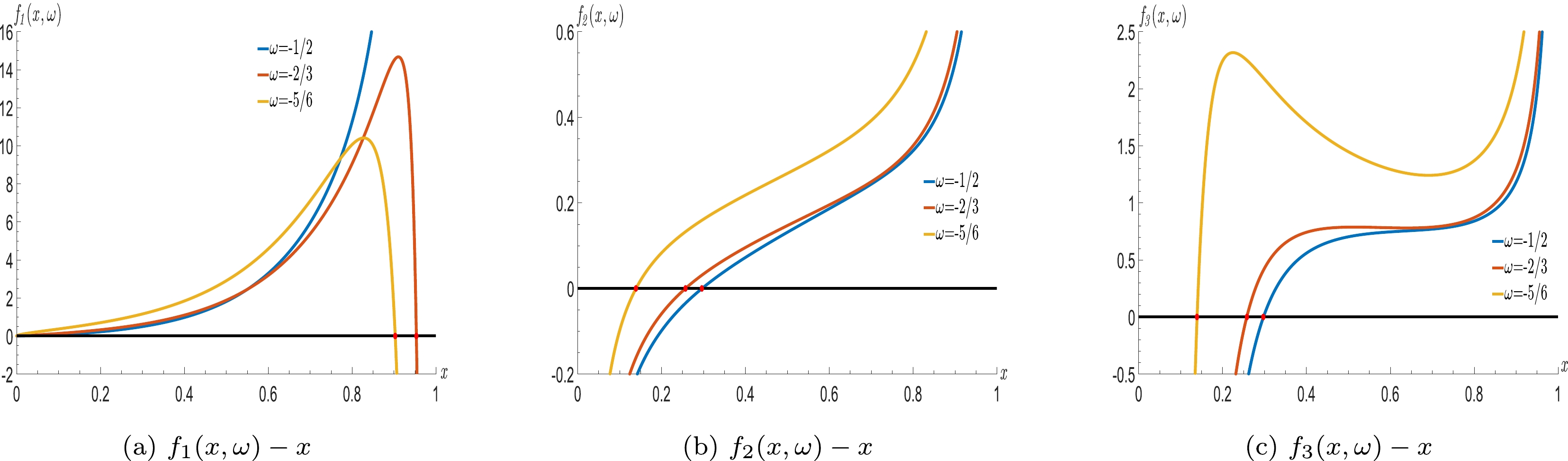
Figure 1. (color online) The behavior of
$ f_{1}(x,\omega) $ ,$ \; f_{2}(x,\omega) $ and$ \; f_{3}(x,\omega) $ as a function of x for different values of ω. -
In this part, we will reconstruct Maxwell's equal-area law in the
$P_{\rm eff}-V$ ,$T_{\rm eff}-S$ planes for the C-dSSQ spacetime and present the condition of phase transition that emerges in C-dSSQ spacetime by adopting different independent dual quantities. -
For the C-dSSQ spacetime with the fixed the ratio x (
$ x_{{\min}}<x<x_{0} $ ) and the temperature$ T_{\rm eff}^{0}\leq T_{\rm eff}^c $ ($ T_{\rm eff}^c $ is the critical temperature),$ V_1,\; V_2 $ and$ P_{\rm eff}^{0} $ denote the horizontal and longitudinal coordinates at the boundary of the two-phase coexistence area in the$ P_{\rm eff}-V $ plane, respectively. From the Maxwell's equal-area law [43, 44, 54−57]$ \begin{eqnarray} P_{\rm eff}^{0}(V_{2}-V_{1})&=&\int_{V_1}^{V_2}P_{\rm eff} {\rm d} V \end{eqnarray} $

(29) and the state equations at two horizon surfaces
$ \begin{aligned}[b] P_{\rm eff}^{0}=\frac{T_{\rm eff}^{0} f_{1}(x,\omega)}{r_1}-\frac{(1-a)f_{2}(x,\omega)}{r_{1}^{2}}+\frac{Q^{2}f_{3}(x,\omega)}{r_{1}^{4}}, \end{aligned} $

$ \begin{aligned}[b] P_{\rm eff}^{0}=\frac{T_{\rm eff}^{0} f_{1}(x,\omega)}{r_2}-\frac{(1-a)f_{2}(x,\omega)}{r_{2}^{2}}+\frac{Q^{2}f_{3}(x,\omega)}{r_{2}^{4}}, \end{aligned} $

(30) one can obtain the following forms
$ \begin{aligned}[b] P_{\rm eff}^{0}\frac{r_{2}^{3}}{3}(1-y^3)=&\frac{T_{\rm eff}^{0}f_{1}(x,\omega)r_2^2(1-y^2)}{2}\\&-(1-a)f_{2}(x,\omega)r_2(1-y)\\&+\frac{Q^2f_{3}(x,\omega)(1-y)}{r_2y}, \\ P_{\rm eff}^{0}\frac{r_2^3}{3}(1+y+y^2)=&\frac{T_{\rm eff}^{0}f_{1}(x,\omega)r_2^2(1+y)}{2}\\&-(1-a)f_{2}(x,\omega)r_2+\frac{Q^2f_{3}(x,\omega)}{r_2y}, \end{aligned} $

(31) where
$ r_1 $ and$ r_2 $ stand for the cosmological horizon positions of two-phase coexistence region, respectively, and$ y=r_{1}/r_{2} $ is the ratio between the cosmological horizon radii of two coexistent phases. From Eq. (30), we have$ \begin{aligned}[b] 0=&\frac{T_{\rm eff}^{0}f_{1}(x,\omega)}{r_{2}y}-\frac{(1-a)f_{2}(x,\omega)(1+y)}{r_{2}^{2}y^{2}}\\&+\frac{Q^{2}f_{3}(x,\omega)(1+y^2)(1+y)}{r_{2}^{4}y^{4}}, \end{aligned} $

(32) $ \begin{aligned}[b] 2P_{\rm eff}^{0}=&\frac{T_{\rm eff}^{0}f_{1}(x,\omega)(1+y)}{r_{2}y}-\frac{(1-a)f_{2}(x,\omega)(1+y^2)}{r_{2}^{2}y^{2}}\\&+\frac{Q^{2}f_{3}(x,\omega)(1+y^4)}{r_{2}^{4}y^{4}}. \end{aligned} $

(33) Combining Eqs. (31) and (33), one can derive
$ \begin{aligned}[b]& \frac{T_{\rm eff}^{0}f_{1}(x,\omega)(1+y)}{r_{2}y}-\frac{(1-a)f_{2}(x,\omega)(1+3y+y^2)}{r_{2}^{2}y^{2}}\\=&-\frac{Q^{2}f_{3}(x,\omega)\big[(1+y+y^2)^{2}+y(1+y)^{2}+y^2\big]}{r_{2}^{4}y^{4}}. \end{aligned} $

(34) From Eqs. (32) and (34), we have
$ \begin{eqnarray} \frac{Q^2}{r_{2}^{2}y^{2}}=(1-a)\frac{f_{2}(x,\omega)}{f_{3}(x,\omega)(1+4y+y^2)}. \end{eqnarray} $

(35) From the above equation, we can see that when
$ y\rightarrow1 $ the critical point position$ r_c^c $ of cosmological horizon of space-time satisfy the following form$ \begin{eqnarray} \frac{Q^2}{{(r_{c}^{c})}^2}=(1-a)\frac{f_{2}(x,\omega)}{6 f_{3}(x,\omega)}. \end{eqnarray} $

(36) Thus, the critical temperature
$T_{\rm eff}^{c}$ and pressure$P_{\rm eff}^{c}$ become$ \begin{aligned}[b] T_{\rm eff}^{c}=&\frac{4(1-a)f_{2}(x,\omega)}{3Qf_{1}(x,\omega)}\left(\frac{(1-a)f_{2}(x,\omega)}{6f_{3}(x,\omega)}\right)^{1/2}, \\ P_{\rm eff}^{c}=&\frac{(1-a)^{2}f_{2}^2(x,\omega)}{12Q^{2}f_{3}(x,\omega)}. \end{aligned} $

(37) From Eqs. (36) and (37) and the fact that the critical quantities must be positive, we can see that when and only when all functions of
$ f_{1}(x,\omega) $ ,$ f_{2}(x,\omega) $ , and$ f_{3}(x,\omega) $ are positive, the requirement of this system can be satisfied. By introducing a parameter χ, which satisfies$T_{\rm eff}^{0}= \chi T_{\rm eff}^{c}$ , it can be expressed as$ \begin{eqnarray} \chi&=&\frac{3y(1+y)\sqrt{6}}{{(1+4y+y^2)}^{3/2}}, \end{eqnarray} $

(38) and from Eq. (38), the corresponding curve of
$ \chi-y $ is presented in Fig. 2 for$ 0<\chi<1 $ .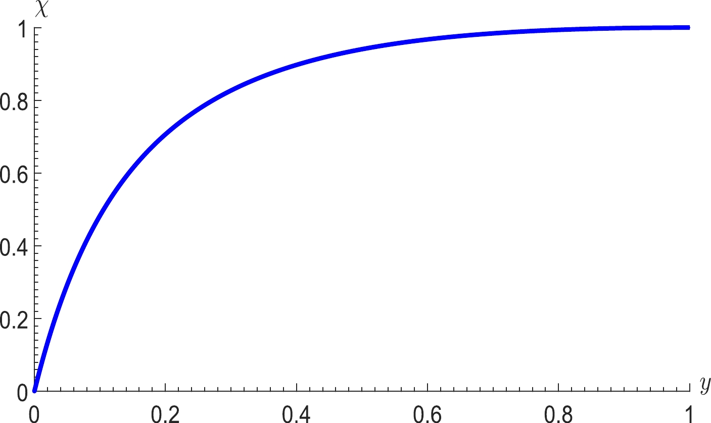
Figure 2. (color online) The behavior of χ as a function of y.
On the other hand, by substituting Eq. (38) into Eq. (27), we can obtain
$ \begin{aligned}[b] P_{\rm eff}=&\chi\frac{4(1-a)f_{2}(x,\omega)}{3Qr_c}\left(\frac{(1-a)f_{2}(x,\omega)}{6f_{3}(x,\omega)}\right)^{1/2} \\&-\frac{(1-a)f_{2}(x,\omega)}{r_{c}^{2}}+\frac{Q^{2}f_{3}(x,\omega)}{r_{c}^{4}}. \end{aligned} $

(39) Combining Eq. (18) and Eq. (39), we exhibit the isotherm process of the
$P_{\rm eff}-V$ phase diagram in Fig. 3 with different parameters χ, x, and ω, respectively. Here, the charge Q is set to$ 1 $ . From Fig. 3(a), it is clearly seen that the behavior of the effective pressure$P_{\rm eff}$ with volume V under the condition of different effective temperature$T_{\rm eff}$ is similar to the$ \it{P-V} $ curve of the vdW system undergoing an isothermal process. Using Maxwell's equal-area law, we also calculate the position of the first-order phase transition. The critical curves with different values of x and ω are shown in Fig. 3(b) and 3(c). The critical pressure increases with the position ratio x between two horizons, while it decreases with the state parameter ω of dark energy. The role of the state parameter ω of dark energy in this system is similar to the attractive interaction between microscopic particles in ordinary thermodynamic systems. Therefore, the increase in ω is similar to the enhancement of attractive interaction between microscopic particles, and the pressure of the system decreases at the same time.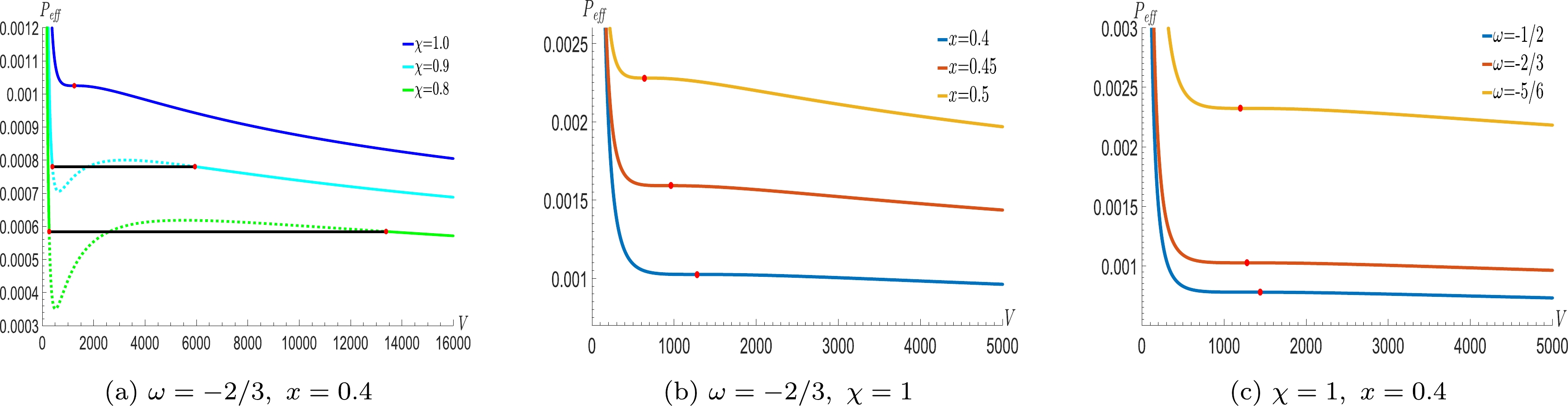
Figure 3. (color online) The behavior of the effective pressure
$P_{\rm eff}$ as a function of V, (a) for different χ, (b) for different x, (c) for different ω.In order to meet the requirements of the stable thermodynamic equilibrium and the positive pressure, the phase trantion temperature exists at the minimum value, which satisfies the following constraints:
$ \begin{eqnarray} \left(\frac{\partial{P_{\rm eff}}}{\partial{V}}\right)_{T_{\rm eff}}=\left(\frac{\partial{P_{\rm eff}}}{\partial{r_{c}}}\right)_{T_{\rm eff}}\left(\frac{\partial{r_{c}}}{\partial{V}}\right)_{T_{\rm eff}}=0,\; \; \; P_{\rm eff}(V,T_{\rm eff})=0. \end{eqnarray} $

(40) From Eq. (40), one can obtain
$ \begin{eqnarray} \frac{Q^2}{{r_{{c\min}}^{2}}}=\frac{(1-a)f_{2}(x,\omega)}{3f_{3}(x,\omega)}. \end{eqnarray} $

(41) Thus, the minimum temperature becomes
$ \begin{eqnarray} T_{\rm eff}^{{\min}}=\frac{2(1-a)f_{2}(x,\omega)}{3Qf_{1}(x,\omega)}\left(\frac{(1-a)f_{2}(x,\omega)}{3f_{3}(x,\omega)}\right)^{1/2}. \end{eqnarray} $

(42) Further, the ratio between the minimum and the critical temperatures reads
$ \begin{eqnarray} \frac{T_{\rm eff}^{\min}}{T_{\rm eff}^{\it{c}}}=\frac{1}{\sqrt{2}}, \end{eqnarray} $

(43) which is a constant and is irrelevant to the position ratio between two horizons. From Eq. (42), we exhibit the corresponding curves of
$T_{\rm eff}^{\min}-x$ with a different state parameter ω in Fig. 4. It is obvious that the minimum effective curve decreases with the decrease in ω, while the minimum value of the ratio when the minimum effective temperature equals zero increases with increase in ω. Thus, the value of ω is not only related to the minimum effective temperature but also to the range of the ratio between two horizons.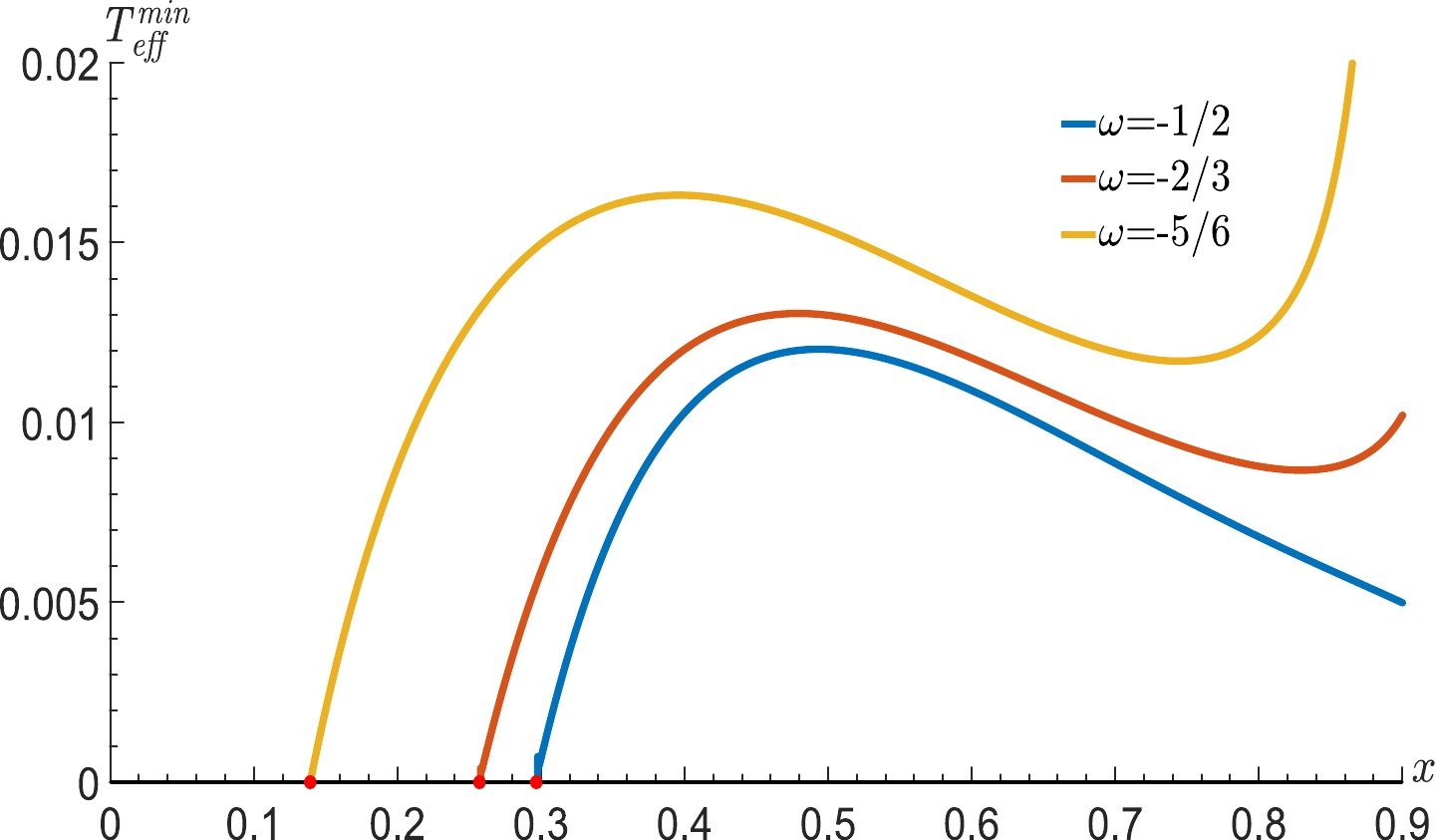
Figure 4. (color online) The behavior of the lowest effective temperature
$T_{\rm eff}^{\min}$ as a function of x for different ω. -
In the following, we will reconstruct Maxwell's equal-area law in the
$T_{\rm eff}-S$ phase diagram. For the C-dSSQ spacetime with a fixed pressure ($P_{\rm eff} < P_{\rm eff}^c$ ) in the equilibrium state, we mark the entropies at the boundary of the two-phase coexistence area as$ S_1 $ and$ S_2 $ , respectively. Then, the corresponding temperature reads$T_{\rm eff}^{0}$ , which is less than the critical temperature$T_{\rm eff}^c$ and is determined by the cosmological horizon radius$ r_c $ . From Maxwell's equal-area law$ \begin{eqnarray} T_{\rm eff}^{0}(S_{2}-S_{1})=\int_{S_1}^{S_2}T_{\rm eff} {\rm d} S \end{eqnarray} $

(44) and the equation of state
$ \begin{aligned}[b] T_{\rm eff}^{0}=&\frac{P_{\rm eff}^{0}r_1}{f_{1}(x,\omega)}-\frac{(1-a)f_{2}(x,\omega)}{r_{1}f_{1}(x,\omega)}-\frac{Q^{2}f_{3}(x,\omega)}{r_{1}^{3}f_{1}(x,\omega)}, \\ T_{\rm eff}^{0}=&\frac{P_{\rm eff}^{0}r_2}{f_{1}(x,\omega)}-\frac{(1-a)f_{2}(x,\omega)}{r_{2}f_{1}(x,\omega)}-\frac{Q^{2}f_{3}(x,\omega)}{r_{2}^{3}f_{1}(x,\omega)}, \end{aligned} $

(45) we can obtain
$ \begin{aligned}[b] T_{\rm eff}^{0}r_{2}^{2}(1+y)=&2\Bigg(\frac{P_{\rm eff}^{0}r_{2}^{3}(1+y+y^2)}{3f_{1}(x,\omega)}+\frac{(1-a)f_{2}(x,\omega)r_{2}}{f_{1}(x,\omega)}\\&-\frac{Q^{2}f_{3}(x,\omega)}{r_{2}yf_{1}(x,\omega)}\Bigg). \end{aligned} $

(46) Note that Eqs. (45) and (46) have the same form as Eqs. (30) and (31), respectively. Therefore, there exists the following expression
$ \begin{eqnarray} T_{\rm eff}^{0}=\frac{P_{\rm eff}^{0}r_{c}}{f_{1}(x,\omega)}+\frac{(1-a)f_{2}(x,\omega)}{r_{c}f_{1}(x,\omega)}-\frac{Q^{2}f_{3}(x,\omega)}{r_{c}^{3}f_{1}(x,\omega)}. \end{eqnarray} $

(47) Combining Eqs. (47) and (21), we show the first-order phase diagram of
$T_{\rm eff}-S$ with different values of pressure and the corresponding critical curves in Fig. 5 with different parameters. On comparing with the results in the last part, we find that the conditions of the first-order phase transition for the C-dSSQ spacetime obtained by adopting different independent dual quantities ($P_{\rm eff}-V$ and$T_{\rm eff}-S$ ) are the same. It shows that any pair of independent dual quantities among the state parameters can be taken as independent variables to discuss the thermodynamic properties of the system, and the corresponding conclusion will not be different, which is due to the fact that a real physical process is independent of the specific description quantities.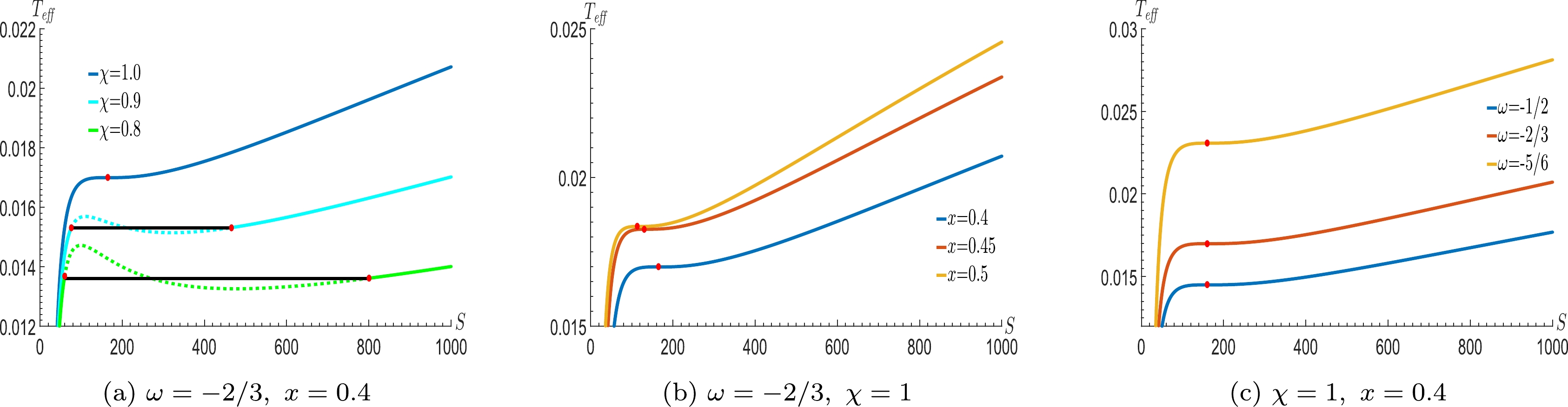
Figure 5. (color online) The behavior of the effective temperature
$T_{\rm eff}$ as a function of S, (a) for different values of pressure, (b) for different values of x and (c) for different values of ω. The charge Q is set to$ 1 $ .Additionally, from Eqs. (35) and (38), we can see that for a given effective temperature
$T_{\rm eff}$ , χ will be fixed, and the phase transition of the C-dSSQ spacetime depends on the cosmological (or black hole) horizon potential, instead of the one between a large black hole and a small black hole. The potential$ \varphi_1 $ at phase$ 1 $ with a small cosmological horizon radius is greater than the potential$ \varphi_2 $ at phase$ 2 $ with a large cosmological horizon radius, i.e.$ \varphi_1>\varphi_2 $ . In fact, for the given effective temperature$T_{\rm eff}$ , the system will be in a two-phase coexistent state when the corresponding potential satisfies$ \varphi_1\geq\varphi\geq\varphi_2 $ , while it will be in a single phase state when the potential satisfies$ \varphi>\varphi_1 $ or$ \varphi<\varphi_2 $ . The system with a potential satisfying$ \varphi>\varphi_1 $ or$ \varphi<\varphi_2 $ corresponds to the liquid or gas phase of the vdW system, respectively, and the system with a potential in the interval of$ \varphi_1\geq\varphi\geq\varphi_2 $ corresponds to the gas-liquid coexistent region. We also show the relation between the potential at the cosmological horizon surface and the state parameter ω when the system is in a two-phase coexistent state as shown in Fig. 6. The function of$\dfrac{Q^2}{r_{2}^{2}}$ is not monotonic with the parameter ω, so there is an unstable maximum as the system is in the two-phase coexistent state, and the potential located at the cosmological horizon surface will reach the minimum value as$ \omega\rightarrow -1 $ . These results indicate that the value of parameter ω has a certain effect on the potential at the cosmological horizon.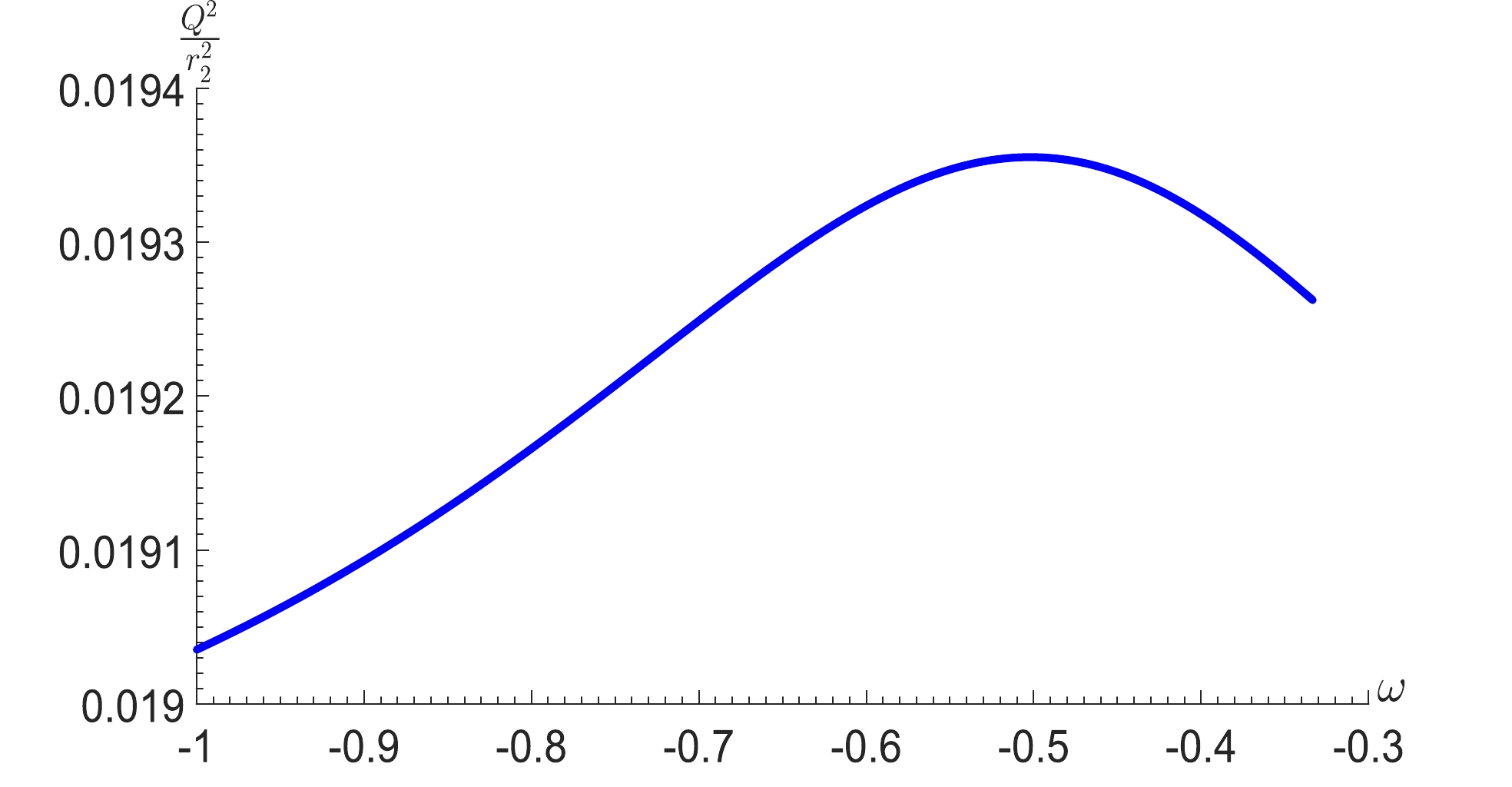
Figure 6. (color online) the behavior of
$ \frac{Q^2}{r_{2}^{2}} $ as a function of$ -1<\omega<-1/3 $ with a = 0, y = 0.9, x = 0.6. -
For an ordinary thermodynamic system in a two-phase (phase
$ 1 $ and phase$ 2 $ ) coexistent state, the coexistent curve of$ P-T $ is determined directly by the experimental verification. Meanwhile, the slope of the$ P-T $ coexistence curve is expressed by the following Clapeyron equation:$ \begin{eqnarray} \frac{{\rm d} P}{{\rm d} T}=\frac{L}{T(V_{2}-V_{1})}, \end{eqnarray} $

(48) where
$ L=T(S_{2}-S_{1}) $ is the latent heat of phase transition,$ V_1 $ and$ V_2 $ stand for the volumes of the system in phase$ 1 $ and phase$ 2 $ , respectively. Using Eqs. (34) and (35), we have$ \begin{eqnarray} T_{\rm eff}^{0}=\frac{(1-a)f_{2}(x,\omega)4y(1+y)}{Qf_{1}(x,\omega)(1+4y+y^2)}\left(\frac{(1-a)f_{2}(x,\omega)}{f_{3}(x,\omega)(1+4y+y^2)}\right)^{1/2}, \end{eqnarray} $

(49) $ \begin{eqnarray} P_{\rm eff}^{0}=\frac{3(1-a)^{2}y^{2}{f_{2}^{2}(x,\omega)}}{Q^{2}f_{3}(x,\omega){(1+4y+y^2)}^{2}}. \end{eqnarray} $

(50) Combining Eqs. (49) and (50), we exhibit the coexistent curve of
$P_{\rm eff}^{0}-T_{\rm eff}^{0}$ with$ Q=1 $ and different parameters (x and ω) in Fig. 7. It demonstrates the effect of the position ratio x on the effective pressure$P_{\rm eff}^{0}$ and temperature$T_{\rm eff}^{0}$ . Fig. 7(a) shows that the effective pressure$P_{\rm eff}^{0}$ increases with x for a given effective temperature$T_{\rm eff}^{0}$ . Fig. 7(b) exhibits the effect of the state parameter ω on the effective pressure$P_{\rm eff}^{0}$ and temperature$P_{\rm eff}^{0}$ . From these figures, we can see that the behavior of the effective pressure is not fully consistent for different values of the parameter x. In general, the effect of the state parameter ω is not distinct for the curve in the$P_{\rm eff}^{0}-T_{\rm eff}^{0}$ diagram.
Figure 7. (color online) The behavior of
$P_{\rm eff}^{0}$ as a function of$T_{\rm eff}^{0}$ , (a) for different x, (b) for different ω.Through Eqs. (49) and (50), the slope of the two-phase coexistent curve in the
$P_{\rm eff}^{0}-T_{\rm eff}^{0}$ plane satisfies$ \begin{eqnarray} \frac{{{\rm d} P_{\rm eff}^{0}}}{{{\rm d} T_{\rm eff}^{0}}}=\frac{3f_{1}(x,\omega)\big[(1-a)f_{2}(x,\omega)f_{3}(x,\omega)\big]^{1/2}}{4Q}\frac{F_{1}'(y)}{F_{2}'(y)}, \end{eqnarray} $

(51) where
$ \begin{eqnarray} F_{1}(y)=\frac{y^2}{(1+4y+y^2)^{2}},\; \; \; F_{2}(y)=\frac{4y(1+y)}{(1+4y+y^2)^{3/2}} \end{eqnarray} $

(52) with
$F_{1}'(y)=\dfrac{{\rm d} F_{1}(y)}{{\rm d} y}$ ,$F_{2}' (y)=\dfrac{{\rm d}F_{2}(y)}{{\rm d}y}$ . From Eqs. (48) and (51), we can obtain the latent heat of phase transition as follows:$ \begin{aligned}[b] L=&\frac{4\pi Q (1+y)(1-y^3)f_{3}(x,\omega)}{y^2}\\&\times\big[(1-a)f_{2}\left(x,\omega\right)f_{3}\left(x,\omega\right)\big]^{1/2}\frac{F_{1}^{\prime}(y)}{F_{2}^{\prime}(y)}. \end{aligned} $

(53) From the above equation, we can exhibit the latent heat of phase transition as the function of x and y with
$ Q=1 $ . The results in Fig. 8 indicate that the latent heat of the first order phase transition is monotonous with y and is increasing with the position ratio x, whereas it decreases with the increase in the parameter ω.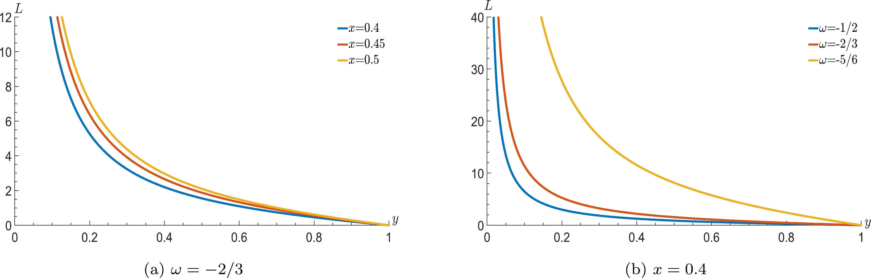
Figure 8. (color online) The behavior of the latent heat L of phase transition as a function of y, (a) for different x, (b) for different ω.
-
Black hole physics, especially black hole thermodynamics, which directly involved physics as well as various fields such as gravitation, statistics, particle physics, and field theory, has attracted considerable attention, and black hole thermodynamics has played an important role in this. Although the precise statistical description of a black hole thermodynamic state is unclear, the black hole thermodynamic property along with the critical phenomenon is still a research subject widely concerned.
In this paper, the continuous phase transition of the C-dSSQ spacetime with a black hole and a cloud of strings and quintessence was analyzed. Using the method of Maxwell's equal-area law, we investigated the condition of phase transition of the C-dSSQ spacetime by adopting different independent dual state parameters
$P_{\rm eff}-V$ and$T_{\rm eff}-S$ . The results indicate that the phase transition conditions for the adoption of different independent dual quantities$P_{\rm eff}-V$ and$T_{\rm eff}-S$ are identical. The independent dual quantities$P_{\rm eff}-V$ and$T_{\rm eff}-S$ are state functions that are independent of the concrete physical process. It provides a way to select the independent dual quantities and establish a theoretical basis to perform an in-depth probe of the critical phenomena of different dS spacetimes. On the other hand, the C-dSSQ has a similar first-order phase transition behavior to that of the vdW system. However, the phase transition is determined by the potential at the cosmological horizon, instead of the pure one between a large and a small black hole. This indicates that the charge plays a key role in the phase transition.For the vdW system, the reason for the phase transition was expounded as the interaction between molecules of the system. However, the major reason for the phase transition of C-dSSQ spacetime is due to the magnitude of electric field subjected by 'molecules' of this system. For the system with a high potential state, i.e. the 'molecules' are in a strong electric field phase arranged orderly under the action of an electric field, the system is in an order phase. Meanwhile, for a low potential phase, the 'molecules' are in a weak electric field phase arranged disorderly under the action of an electric field, the system is in a disorder phase. The 'molecules' affected by the thermal fluctuations and electric field are in the phase transition region from disorder to order or from order to disorder when the system is in the two-phase coexistent state. Additionally, we found that the parameter ω has a certain effect on the potential at the cosmological horizon, and when the system is in a two-phase coexistent state, the potential at the cosmological horizon as the function of x has an unstable maximum; in particular, it will arrive at the minimum as
$ \omega\rightarrow -1 $ . The coexistent curves indicated that the phase transition pressure and temperature are both increasing with x. Meanwhile, the parameter ω has little effect on the coexistent curves. The latent heat of the first order phase transition increases with the position ratio x, while it decreases with the parameter ω.This work revealed the microstructure and the effect of state parameter ω on the phase transition of the C-dSSQ spacetime with a black hole and a cloud of strings and quintessence. These conclusions provide specific guidance for exploring the microstructure of a black hole. In particular, further research of the microstructure of a black hole is helpful to understand the basic properties of black hole gravity, which is also important for the establishment of quantum gravity.
-
We would like to thank Prof. Ren Zhao and Meng-Sen Ma for their indispensable discussions and comments.
Continuous phase transition of the de Sitter spacetime with charged black holes and cloud of strings and quintessence
- Received Date: 2023-07-19
- Available Online: 2023-11-15
Abstract: Recently, some meaningful results have been obtained by studying the phase transition, critical exponents, and other thermodynamical properties of different black holes. Especially for the Anti-de Sitter (AdS) black holes, their thermodynamical properties nearby the critical point have attracted considerable attention. However, there exists little work on the thermodynamic properties of the de Sitter (dS) spacetime with black holes. In this paper, based on the effective thermodynamical quantities and the method of the Maxwell's equal-area law, we explore the phase equilibrium for the de Sitter spacetime with the charged black holes and the cloud of string and quintessence (i.e., C-dSSQ spacetime). The boundaries of the two-phase coexistence region in both


 DownLoad: