


 Abstract
 HTML
HTML Reference
 Related
 PDF
PDF


-
The recent acceleration of the expansion of the universe is entirely supported by different observations [1, 2]. This phenomenon is supported by the increase in observational evidence such as cosmic microwave background (CMB) anisotropies [3−6], baryon acoustic oscillation (BAO) [7, 8], Hubble parameters derived from passively evolving galaxies [9, 10], and Einstein radius measurements of strong lensing systems [11, 12]. The explanation behind the late-time acceleration of universe expansion is one of the most important topics in cosmology and is completely supported by different observations. It requires the assumption of an effectively perfect fluid that violates several energy conditions, known as dark energy (DE) [13, 14]. To achieve acceleration, the universe should be dominated by exotic fluid with negative pressure. The cosmological constant Λ, in which the equation of state (EoS) parameter is equal to
$ -1 $ , is the most likely possibility for DE. A model of the accelerated expansion of the universe is constructed assuming the cosmological constant and cold dark matter (CDM) in the context of standard ΛCDM cosmology. This model confirms the cosmological observations and suffers from serious problems of cosmic coincidence and fine tuning [15, 16]. Other types of cosmological constants based on DE are scalar fields, such as the quintessence field, modified gravity, and phantom DE [17−19].The presence of dynamic DE is a viable alternative to the cosmological constant that is constrained by observational data [20−22]. The phenomenological approach to this issue is expressed by introducing the EoS
$ w(t) $ , which is variable with respect to time and redshift$ (z) $ . The EoS parameter describes the underlying scalar field and its relevant dynamics. Functional forms of$ w(z; w_0, w_1) $ involving a small number of parameters are the infrastructure behind variations in the EoS parameter$ w(z) $ . Numerous such parameterizations have been proposed in literature, such as Chevallier-Polarski-Linder (CPL) parameterization [23], the Jassal-Bagla-Padmanabhan (JBP) model [24, 25], the Barboza-Alcaniz (BA) model [26, 27], and the logarithmic model [28]. The values of the parameters$ (w_0,w_1) $ with the best fit of observational data are provided for each model.The idea that the geometry of the universe at the end of the inflationary era is homogeneous and isotropic is supported by several studies. The Friedman-Robertson-Walker (FRW) model plays an important role in this period [29]. Deficiencies in the CMB reveal an anisotropic phase that then transforms into an isotropic phase. These deficiencies are the result of quantum fluctuations in the inflation period. Thus, anisotropy will be found behind the evolving process. Anisotropy and spatial homogeneity in cosmology are interesting subjects for cosmologists. Some important applications of DE models in the scope of anisotropic Bianchi space-times are given in Refs. [29−39]. Among the Bianchi type models, the Bianchi type I (BI) cosmological model has received the most attention owing to its fundamental properties. It has more degrees of freedom characterized by lie groups. The BI model recovers isotropy as special cases and permits a small amount of anisotropy at some instant of cosmic time. In recent years, many researchers have constructed interesting cosmological models in the presence of DE within the background of anisotropic Bianchi space-times. Recently, Hossienkhani et al. constructed the BI model with interacting holographic and new agegraphic scalar field models of DE [40]. Some useful applications of Bianchi type models compatible with astrophysical observations are given in Refs. [41−45]. The observational datasets include the latest Pantheon sample [46] of type Ia supernovae (SNIa), estimations of the Hubble parameter H(z) data, and their joint combination. The best fits for the free parameters of the parameterization of the EoS parameter (
$ w(z) $ ) in the BI model are applied using the maximum likelihood estimation method and then compared with those of the ΛCDM model. Using this parameterization with current datasets, we can test the generic evolution of the EoS of the acceleration mechanism.In this paper, we consider the parameterization of the EoS parameter and obtain an explicit solution to the Einstein field equations in flat BI space-time. This paper is organized as follows. In the next section, the theoretical model and its basic equations in an anisotropic universe are given. The data samples and characteristic
$ \chi^2 $ for each are obtained in Section III. In Section IV, we present our result for the constraint on the BI universe for parameterizations of the DE EoS. In the final section, we give the conclusion and discussion. -
In this study, we investigate a cosmological model in the context of spatially homogeneous BI space-time, which is given as follows:
$ \begin{equation} {\rm d} s^2={\rm d}t^{2}-A^{2}(t){\rm d}x^{2}-B^{2}(t){\rm d}y^{2}-C^{2}(t){\rm d}z^{2}, \end{equation} $

(1) where A, B, and C are the directional scale factors, which are functions of the cosmic time t alone. Thus, the average scale factor is given by
$ a=(ABC)^{1/3} $ . If we consider the matter field to consist of dark matter (DM) and DE, then the field equations in the BI model are given by$ \begin{equation} R_{ij}-\frac{1}{2}Rg_{ij}=\frac{1}{M_p^2}(T^m_{ij}+T_{ij}^\mathrm{de}), \end{equation} $

(2) where
$ T^m_{ij} $ and$ T_{ij}^\mathrm{de} $ are the energy momentum tensor for DM and DE, respectively, and$ M^2_P=\dfrac{1}{8\pi G} $ is the reduced Planck mass.The energy conservation equation reads as
$ \begin{equation} (T^m_{ij}+T_{ij}^\mathrm{de})_{;\; j}=0. \end{equation} $

(3) Equation (3) leads to
$ \begin{eqnarray} \dot{\rho}_m+\dot{\rho}_\mathrm{de}+3H\rho_m+3H(1+\omega_\mathrm{de})\rho_\mathrm{de}=0, \end{eqnarray} $

(4) where
$ \rho_m $ and$ \rho_\mathrm{de} $ are the energy density of DM and DE, respectively,$ \omega_\mathrm{de}=p_\mathrm{de}/\rho_\mathrm{de} $ is the EoS parameter of DE, the over dot denotes derivatives with respect to time (t), and H is the mean Hubble function, defined as$ H=\dot{a}/a $ , with a as the average scale factor. Now, the mean Hubble parameter in BI space-time is given by$ H=\frac{1}{3}(H_1+H_2+H_3)=\frac{1}{3}\left(\frac{\dot{A}}{A}+\frac{\dot{B}}{B}+\frac{\dot{C}}{C}\right), $

(5) where
$ H_1=\dot{A}/A $ ,$ H_2=\dot{B}/B $ , and$ H_3=\dot{C}/C $ are directional Hubble parameters. The scalar expansion and shear scalar can be defined as$ \theta=u^i_{;i}=\frac{\dot{A}}{A}+\frac{\dot{B}}{B}+\frac{\dot{C}}{C}, $

(6) $\sigma^2=\frac{1}{2} \sigma_{ij}\sigma^{ij}=\frac{1}{2}\left( \left(\frac{\dot{A}}{A}\right)^{2}+ \left(\frac{\dot{B}}{B}\right)^{2}+\left(\frac{\dot{C}}{C}\right)^{2} \right )-\frac{1}{6}\theta^{2}, $

(7) where
$ \sigma_{ij}=u_{(i;j)}-\dot{u}_{(i }u_{j)}-\dfrac{1}{3}\theta h_{ij} $ is the shear tensor,$ h=g_{ij}-u_i u_j $ is the projection tensor, and$ u_i=(1, 0, 0, 0) $ is the four-velocity in the comoving coordinates. In the comoving coordinate system, considering Eqs. (5)−(7), the field in Eq. (2) for metric (1) is written as follows [47−49]:$ \begin{eqnarray} &&3H^2-\sigma^2=\frac{1}{M_p^2}(\rho_{m}+\rho_{\rm de}), \end{eqnarray} $

(8) $ \begin{eqnarray} &&2\dot{H}+3H^2+\sigma^2=-\frac{1}{M_p^2}(\rho_{\rm de}\omega_{\rm de}). \end{eqnarray} $

(9) Considering the particular case
$ \sigma=0 $ (implying$A(t) \rightarrow B(t)\rightarrow C(t)$ in (7)),$ \; A(t)=B(t)=C(t)=a(t) $ , the field equation is re-obtained in the framework of the flat FRW metric. Now, by introducing the density parameters$ \Omega_i $ for matter, DE, and anisotropy of the universe, we obtain$ \begin{eqnarray} \Omega_{m}=\frac{ \rho_{m}}{3M_p^2 H^2},\; \; \Omega_{\rm de}=\frac{ \rho_{\rm de}}{3M_p^2 H^2},\; \; \Omega_{\sigma}=\frac{\sigma^2}{3 H^2}. \end{eqnarray} $

(10) Note that the continuity equation for anisotropy can be written as
$ \begin{eqnarray} \dot{\sigma}+3H\sigma=0, \end{eqnarray} $

(11) which in turn gives
$ \begin{eqnarray} \sigma=\sigma_0 a^{-3}, \end{eqnarray} $

(12) where
$ \sigma_0 $ is the constant of integration. This shows that for smaller a, the shear scalar can increase faster and for large quantities, leans to zero. This indicates that at a late time, the universe can seem isotropic like. Because the stiff or Zeldovich fluid is included in the base ΛCDM model, the shear scalar$ \sigma^2 $ contributes to the BI equation as a stiff fluid$ \rho_\sigma\propto a^{-6} $ , described by the EoS of the form$ \omega_\sigma=1 $ . Moreover, the observations of redshift survey place the limit as$ \sigma/H\leq0.3 $ in the neighborhood of our present day galaxy. Collins et al. [50] concluded that for spatially homogeneous space-time, the normal congruence to homogeneous expansion follows the above condition, where$ \sigma/H $ is constant.Owing to the lack of complete knowledge on DE, one way to analyze models on the other side of the cosmological constant is to parameterize the EoS parameter
$ w(z) $ . To do this, we consider the simplest parameterization of the EoS parameter of DE, given by [51, 52]$ \begin{eqnarray} \omega(z)=\frac{\omega_0}{1+z}, \end{eqnarray} $

(13) where
$ \omega_0 $ denotes the present value of the EoS parameter of DE. The main reason for considering the parameterization of$ \omega(z) $ in the form of Eq. (13) is that at$ z=0 $ , it gives$ \omega(0)=\omega_0 $ and obtains ($ z\rightarrow \infty $ ),$ \omega(\infty)\sim0 $ at early times, which is eventually true when modeling the universe. The best fit value of$ \omega_0 $ to gold SNIa, SDSS, and WMAP datasets is$ \omega_0=-1.1 $ [51]. Hence, the parameter favors DE of phantom origin. From the energy conservation law (4),$ \dot{\rho}_{m}+3H(\rho_{m}+p_{m})=0 $ holds for barotropic matter. For the dust filled current universe "$ p_m=0 $ " and using the relation$ 1+z=1/a $ , we get$ \rho_m=\rho_{m_0}(1+z)^3 $ . The conservation law for the DE model is$ \dot{\rho}_\mathrm{de}+3H(1+\omega_\mathrm{de}(z))\rho_\mathrm{de}=0 $ . Therefore, the DE density$\rho_{\rm de}$ is written as$ \rho_{\rm de}=\rho_0 \exp\left[3\int_0^z\left( \frac{1+\omega(z')}{1+z'}\right) {\rm d}z'\right], $

(14) where
$ \omega(z') $ is that given by Eq. (13). From Eq. (14), we can deduce that the evolution of the DE component is highly dependent on the form of its EoS parameter$ \omega(z') $ . Combining Eqs. (13) and (14), the DE density is given as$ \rho_{\rm de}=\rho_0(1+z)^3 \exp\left(\frac{3\omega_0 z}{1+z}\right). $

(15) For
$ z\gg 1 $ , we see that$\rho_{\rm de}\sim\rho_0(1+z)^3 {\rm e}^{3\omega_0}$ and$\rho_{\rm de}\rightarrow \infty$ when$ z\rightarrow -1 $ . Now, substituting$ \rho_m $ ,$\rho_{\rm de}$ , and$ \sigma^2 $ into Eq. (10), we get$ \begin{aligned}[b] \Omega_{m}=&\Omega_{m_0}(1+z)^3\left(\frac{ H_0}{H}\right)^2,\\ \Omega_{\rm de}=&\Omega_{ de_0}(1+z)^3 \exp\left(\frac{3\omega_0 z}{1+z}\right)\left(\frac{ H_0}{H}\right)^2,\\ \Omega_{\sigma}=&\Omega_{\sigma_0}(1+z)^6\left(\frac{ H_0}{H}\right)^2, \end{aligned} $

(16) where
$ H_0 $ is the current Hubble parameter,$\Omega_{m_0}=\rho_{m_0}/ 3M_p^2H^2_0$ is the density parameter for the matter content,$ \Omega_{de_0}=\rho_{de_0}/3M_p^2H^2_0 $ is the density parameter for DE, and$ \Omega_{\sigma_0}=\sigma^2_0/3H^2_0 $ is the density parameter for the anisotropy of the present universe. Using Eqs. (9), (10), and (16) leads to$ \begin{aligned} H^2(z)=&H_0^2\bigg[\Omega_{m_0}(1+z)^3+\Omega_{\sigma_0} (1+z)^6\\&+(1-\Omega_{m_0}-\Omega_{\sigma_0}) (1+z)^3 {\rm e}^{\textstyle\frac{3\omega_0 z}{1+z}}\bigg]. \end{aligned} $

(17) The term
$ \Omega_{\sigma_0} (1+z)^6 $ is the fastest growing term in the average expansion rate as it increases with increasing average redshift z. Notice that the ΛCDM model is recovered for$ \omega_0=0 $ . We also note that$ \Omega_{m_0}+\Omega_{de_0}= 1-\Omega_{\sigma_0} $ . This states that if the shear tensor tends toward zero, the sum of the energy density parameters approaches$ 1 $ at late times. -
The property of ΛCDM and parameterization of the EoS of the DE model is investigated using the best fit value for the model parameters
$ \Omega_{m_0} $ ,$ \Omega_{\sigma_0} $ ,$ \omega_{0} $ , and M in an anisotropic universe. In what follows, we describe the database used. -
A Pantheon sample with a set of the latest data points for the apparent magnitude of SNIa in the range
$ 0.01< z<2.26 $ is used as one of two data point samples in this study [46]. This sample includes 279 spectroscopically confirmed SNIa discovered by the Pan-STARRS1(PS1) Medium Deep Survey [46, 53], Sloan Digital Sky Survey (SDSS) [54, 55], and Supernova Legacy Survey (SNLS) [56, 57]. We compute the residuals$ \Delta \mu $ and minimize the quantity$ \begin{eqnarray} \chi^2_\mathrm{SN}=\Delta \mu^\mathrm{T}. {Cov}^{-1}.\Delta \mu, \end{eqnarray} $

(18) where
$ \Delta\mu\equiv \mu^\mathrm{obs}-\mu^\mathrm{th} $ ,$ {Cov} $ is the covariance matrix,$ \mu^\mathrm{obs} $ is taken from the compilation presented in [46], and the$\mu^{\rm th}$ distance modulus of the luminosity distance is estimated, which is defined as$ \begin{equation} \mu(z_i)=M+5\log_{10}\bigg[(1+z)H_0\int^z_0 {\rm d} z'H^{-1}(z')\bigg]+25, \end{equation} $

(19) where M represents the absolute B-band magnitude of a fiducial SNIa, and
$ H(z) $ contains the free parameters of Eq. (17). From Eq. (19), we can easily see a degeneracy between the parameters M and$ H_0 $ , which is considered constant in the context of a DE model$ H(z) $ . Therefore, if we take M to be a member of the set of nuisance parameters characterizing the SN luminosities, the parameterization of the EoS of the DE model will have, at most, only three parameters:$ \Omega_{m_0} $ ,$ \Omega_{\sigma_0} $ , and$ \omega_{0} $ . For consistency with Refs. [46, 58], we set$ H_0 =70\; \mathrm{km \; s^{-1} Mpc^{-1}} $ . -
The Hubble dataset with 52 data points in the redshift range
$ 0\leq z\leq2.36 $ is extracted in this study (see Table 1). Out of the 52 Hubble data points, 30 points are measured via the method of differential age (DA). BAO and another method are applied to extract the remaining 22 points. Table 1 shows the 52 H(z) points used in this paper and Refs. [59−61]. To find the best fit value of the parameters of the obtained models, we use the technique of a$ \chi^2 $ -test defined by the following statistical formula:z $H(z) $ 

$\sigma'_{H^{\rm obs}(z)}$ 

z $H(z) $ 

$\sigma'_{H^{\rm obs}(z)}$ 

$0$ 

$73.24$ 

$1.74$ 

$0.07$ 

$69$ 

$19.6$ 

$0.1$ 

$69$ 

$12$ 

$0.12$ 

$68.6$ 

$26.2$ 

$0.17$ 

$83$ 

$8$ 

$0.1791$ 

$75$ 

$4$ 

$0.1993$ 

$75$ 

$5$ 

$0.2$ 

$72.9$ 

$29.6$ 

$0.24$ 

$79.69$ 

$2.65$ 

$0.27$ 

$77$ 

$14$ 

$0.28$ 

$88.8$ 

$36.6$ 

$0.3$ 

$81.7$ 

$6.22$ 

$0.31$ 

$78.17$ 

$4.74$ 

$0.35$ 

$82.7$ 

$8.4$ 

$0.3519$ 

$83$ 

$14$ 

$0.36$ 

$79.93$ 

$3.39$ 

$0.38$ 

$81.5$ 

$1.9$ 

$0.3802$ 

$83$ 

$13.5$ 

$0.4$ 

$95$ 

$17$ 

$0.4004$ 

$77$ 

$10.2$ 

$0.4247$ 

$87.1$ 

$11.2$ 

$0.43$ 

$86.45$ 

$3.68$ 

$0.44$ 

$82.6$ 

$7.8$ 

$0.4497$ 

$92.8$ 

$12.9$ 

$0.47$ 

$89$ 

$34$ 

$0.4783$ 

$80.9$ 

$9$ 

$0.48$ 

$97$ 

$60$ 

$0.51$ 

$90.4$ 

$1.9$ 

$0.52$ 

$94.35$ 

$2.65$ 

$0.56$ 

$93.33$ 

$2.32$ 

$0.57$ 

$96.8$ 

$3.4$ 

$0.59$ 

$98.48$ 

$3.19$ 

$0.5929$ 

$104$ 

$13$ 

$0.6$ 

$87.9$ 

$6.1$ 

$0.61$ 

$97.3$ 

$2.1$ 

$0.64$ 

$98.82$ 

$2.99$ 

$0.6797$ 

$92$ 

$8$ 

$0.73$ 

$97.3$ 

$7$ 

$0.7812$ 

$105$ 

$12$ 

$0.8754$ 

$125$ 

$17$ 

$0.88$ 

$90$ 

$40$ 

$0.9$ 

$117$ 

$23$ 

$1.037$ 

$154$ 

$20$ 

$1.3$ 

$168$ 

$17$ 

$1.363$ 

$160$ 

$33.6$ 

$1.43$ 

$177$ 

$18$ 

$153$ 

$140$ 

$14$ 

$1.75$ 

$202$ 

$40$ 

$1.965$ 

$186.5$ 

$50.4$ 

$2.33$ 

$224$ 

$8$ 

$2.34$ 

$222$ 

$7$ 

$2.36$ 

$226$ 

$8$ 

Table 1. Hubble parameter
$H(z)$ with redshift and errors$\sigma'_i$ .$ \begin{eqnarray} \chi^2_{H(z)}=\sum_{n=1}^{52} \frac{[(H_i)_\mathrm{th}(z)-(H_i)_\mathrm{obs}(z)]^2}{\sigma'^2_{(H_i)_\mathrm{obs}(z)}}, \end{eqnarray} $

(20) where
$ (H_i)_\mathrm{obs} $ and$ (H_i)_\mathrm{th} $ are the observed and predicted values of the Hubble parameter, respectively. -
In our examination, the different measurements of SNIa and H(z) are merged by adding their corresponding
$ \chi^2 $ functions. They are not all dependent on each other and explore different cosmic periods. We express the combination of all the data as$ \begin{eqnarray} \chi^2_\mathrm{Total}=\chi^2_\mathrm{SNIa}+\chi^2_ {H(z)}, \end{eqnarray} $

(21) where each function is defined as explained in previous subsections.
-
Now, we are ready to apply the maximum likelihood technique [62] using the effects of anisotropy on the aforementioned DE models. A cosmological model with a standard DM and DE component, considering the parameterization Eq. (13) with
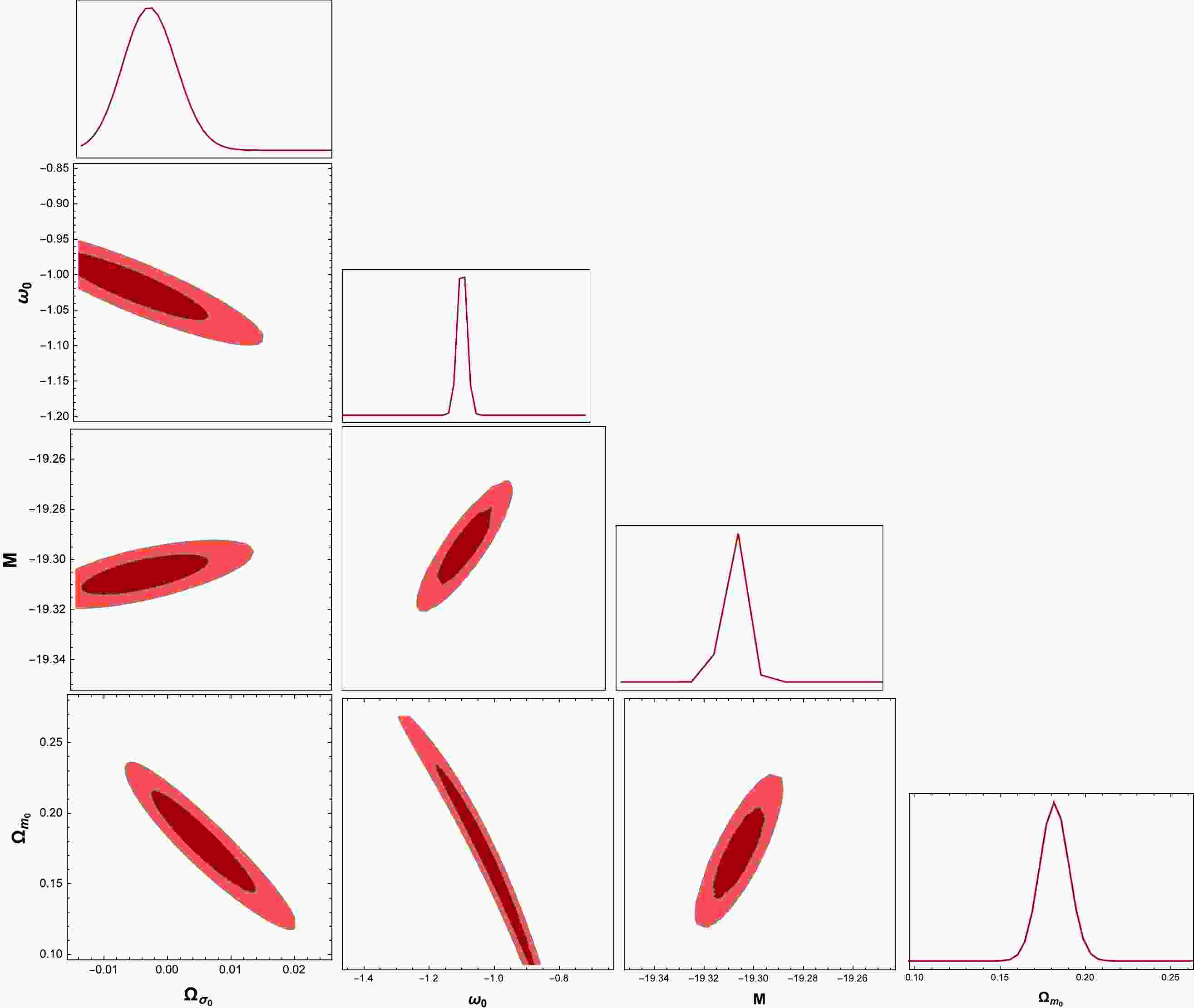
$ H(z) $ defined in (17), is considered. A statistical method based on MLE is developed to minimize the$ \chi^2 $ estimator with reduced chi-squared,$\chi^2_{\rm red}= \chi^2_{\rm min}/(d.o.f.)$ . In addition to the MLE technique, a prior technique on the Hubble parameter tension$H_0 =70 \mathrm{km \; s^{-1} Mpc^{-1}}$ is established, as cited in Refs. [46, 58]. We depict two dimensional contours in the$ 1\sigma' $ and$ 2\sigma' $ confidence regions by bounding our model with Pantheon and Pantheon+H(z) data, which is shown in Figs. 1 and 2. The results of this analysis are summarized in Table 2.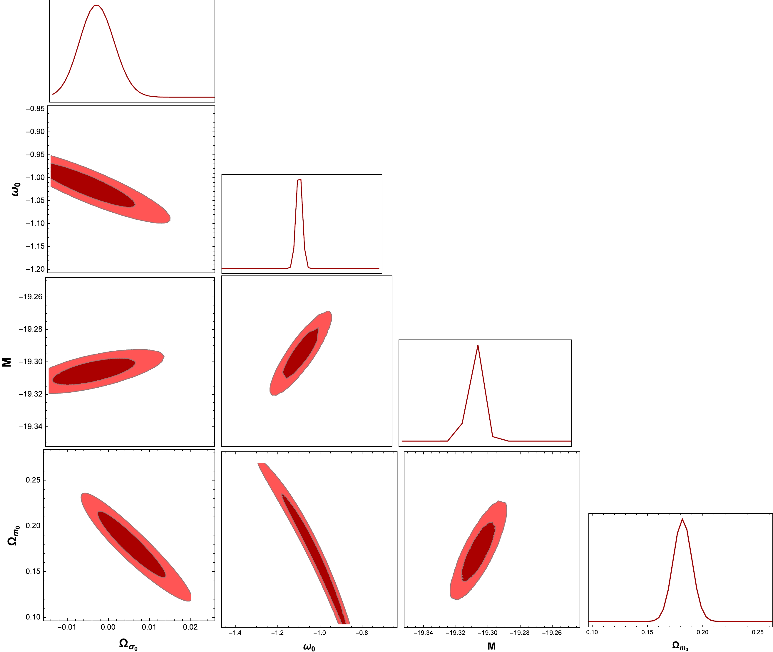
Figure 1. (color online) One-dimensional posterior distributions and two-dimensional marginalized contours (
$ 1\sigma' $ and$ 2\sigma' $ ) for the parameters$ \Omega_{m_0} $ ,$ \Omega_{\sigma_0} $ ,$ \omega_0 $ , and M in the parameterization of the DE model ($ \omega=\omega_0/(1+z) $ ) using the Pantheon data for$ H_0 =70\; \mathrm{km \; s^{-1} Mpc^{-1}} $ prior.ΛCDM model Parameterization of the DE model Parameters Pantheon data Pantheon+H(z) data Pantheon data Pantheon+H(z) data $\Omega_{m_0}$ 

$0.229\pm0.038$ 

$0.286\pm0.009$ 

$0.181\pm0.221$ 

$0.285\pm0.055$ 

$\Omega_{\sigma_0}$ 

$0.01098\pm0.00749$ 

$-0.00078\pm0.00041$ 

$0.00503\pm0.01341$ 

$-0.00183\pm0.00091$ 

M $-19.298\pm0.008$ 

$-19.291\pm0.005$ 

$-19.306\pm0.012$ 

$-19.312\pm0.009$ 

$\omega_0$ 

$-$ 

$-$ 

$-1.013\pm0.339$ 

$-1.205\pm0.165$ 

$\chi^2_{min}$ 

$1007.02$ 

$1039.38$ 

$1006.14$ 

$1033.52$ 

$\chi^2_{\rm red}$ 

$0.963$ 

$0.947$ 

$0.964$ 

$0.943$ 

Table 2. Best fit values of the cosmological parameters for the ΛCDM (left) and parameterization of the DE model (
$\omega=\omega_0/(1+z)$ ) (right) in an anisotropic universe for$H_0 =70\; \mathrm{km \; s^{-1} Mpc^{-1}}$ prior.
Figure 2. (color online) One-dimensional posterior distributions and two-dimensional marginalized contours (
$ 1\sigma' $ and$ 2\sigma' $ ) for the parameters$ \Omega_{m_0} $ ,$ \Omega_{\sigma_0} $ ,$ \omega_0 $ , and M in the parameterization of the DE model ($ \omega=\omega_0/(1+z) $ ) using the Pantheon+H(z) data for$ H_0 =70\; \mathrm{km \; s^{-1} Mpc^{-1}} $ prior.Considering the standard ΛCDM scenario with the Pantheon sample, we obtain
$ \Omega_{m_0}=0.229\pm0.038 $ and$ M=-19.298\pm0.008 $ (see the first row of Table 2). Given the SNLS sample for the ΛCDM model, Guy et al. obtained$ \Omega_{m_0}=0.215 $ and$ M=-19.21 $ , which are compatible with current observational data [63]. By combining the Pantheon data with the H(z) data for ΛCDM in the BI model, we obtain$ \Omega_{m_0}=0.286\pm0.009 $ and$M=-19.291 \pm0.005$ . From Table 2, we find that the smallest value of the reduced$\chi^2_{\rm red}$ belongs to the parameterization of the DE model with the Pantheon+H(z) data.Considering the fit results of the parameterization of the DE model with the Pantheon and Pantheon+H(z) datasets, it is realized that for the parameterization of the DE model, the value of the best fit obtained for
$ \Omega_{m_0} $ is approximately equal to$ \Omega_{m_0}=0.181 $ (for Pantheon+H(z)$ \Omega_{m_0}=0.285 $ ). Then, the fit value of$ \Omega_{m_0} $ in the parameterization of the DE model in the BI model is confirmed with the ΛCDM model using the data combinations. The nuisance parameter is constrained as$M=-19.306,\; -19.312$ with the Pantheon and combined H(z)+Pantheon data, which is in agreement with the results of Ref. [46], where anisotropy cosmology was not considered. With regard to the SNIa and H(z) data in our analysis, we apply the constraint$ \Omega_{\sigma_0}<10^{-3} $ . A comparison with the direct-model independent observational data shows that the method used is appropriate [35, 44].Having obtained the SNIa data, we have
$\omega_0= -1.013\pm0.339$ at the$ 1\sigma' $ confidence level. By combining the H(z) and Pantheon datasets, the parameterization of the DE model approach leads to$ \omega_0=-1.205\pm0.165 $ at the$ 1\sigma' $ confidence level, as shown in Fig. 2. We derive$ -1.25<\omega_0<-1.16 $ at the 95% confidence level, which indicates that DE completely varies in the phantom region. Now, we compare this result with the best fit of the$ \omega_0 $ value obtained with the SNIa 'gold set'+SDSS+ WAMP,$ \omega_0=-1.1\pm0.2 $ [51] and the 159 SNIa data,$ \omega_0 =-1.15^{+0.20}_{-0.17} $ [64]. We find that the values of$ \omega_0 $ , when combined, are consistent with observational values.In the following, we discuss the improvement in the precision of cosmological parameters with the addition of the H(z) data. For the ΛCDM model, the precision of
$ \Omega_{m_0} $ from the data of Pantheon and Pantheon+H(z) are promoted from$16.6\%$ and$ 3.15\% $ , respectively. In the precision of$ \Omega_{\sigma_0} $ , the data of Pantheon and Pantheon+H(z) are improved from$ 68.2\% $ and$ 52.6\% $ , respectively. The precision of M is improved by$ 0.04\% $ and$ 0.02\% $ for the Pantheon and Pantheon+H(z) data, respectively. We can see a more precise nature of the Pantheon+H(z) data compared to the Pantheon data alone. For the parameterization of DE in the BI model, in the current combined observations (Pantheon+H(z)), the constraints on$ \Omega_{m_0} $ ,$ \Omega_{\sigma_0} $ , M, and$ \omega_0 $ are improved by$ 19.3\% $ ,$ 49.7\% $ ,$ 0.04\% $ , and$ 13.7\% $ , respectively. In addition, upon closer examination of the posteriors of Figs. 1 and 2, it is evident that the parameters from the dataset combinations that include Pantheon+H(z) exhibit tighter constraints, with the cosmological parameter showing notably improved precision. Therefore, we conclude that the Pantheon data do not help to improve the constraints on the parameterization of DE in an anisotropic universe; however, they would significantly improve the constraints on the parameterization of DE using the H(z) combination.Because of the different numbers of parameters, a model with more parameters is more favorable with a lesser value of
$ \chi^2 $ . Therefore, we use the Akaike information criterion (AIC) to make a fair model comparison. The selection function of the AIC model can be written as [65, 66]$ \begin{equation} AIC=-2\ln \mathcal{L}_\mathrm{max}+2k+\frac{2k(k+1)}{N_\mathrm{tot}-k-1}, \end{equation} $

(22) where
$ \mathcal{L}_\mathrm{max} $ and k are the maximum likelihood and number of parameters, respectively. For Gaussian errors,$\chi^2_{\min}=-2\ln \mathcal{L}_\mathrm{max}$ . In the case of numerous data points$ N_\mathrm{tot} $ , we have$ AIC\simeq-2\ln \mathcal{L}_\mathrm{max}+2k $ . In actuality, the relative values in various models are more applicable and valuable, i.e., we have$\Delta AIC=\Delta \chi^2_{\min}+2\Delta k$ . A model with a lower AIC value is preferred. In comparison with a reference model, models with$ 0<\Delta AIC<2 $ have considerable support, models with$ 4<\Delta AIC<7 $ have significantly less support, and models with$ \Delta AIC>10 $ have mainly no support [65]. However, compared with the base ΛCDM model with$ \chi^2=1007.02 $ , the parameterization of the DE model has$ \Delta \chi^2=-0.88 $ and$ \Delta AIC=1.12 $ , indicating that the parameterization of DE is favored by the Pantheon data. From a statistical point of view, the parameterization of the DE model has$ \Delta \chi^2=-5.86 $ and$ \Delta AIC=3.86 $ and is considerably less supported by the Pantheon+H(z) data combination (see Table 3).Fit k $\chi^2_\mathrm{min}$ 

AIC $\Delta AIC$ 

ΛCDM model Pantheon 3 1007.02 1013.04 $-$ 

Pantheon+H(z) 3 1039.38 1045.4 $-$ 

$\omega=\omega_0/(1+z)$ 

Pantheon 4 1006.14 1014.18 1.12 Pantheon+H(z) 4 1033.52 1041.56 3.86 Table 3. Minimum value of
$\chi^2$ , AIC, and$\Delta AIC$ of the ΛCDM and parameterization of DE$(\omega=\omega_0/(1+z))$ models in an anisotropic universe using the Pantheon and Pantheon+H(z) data.A distance modulus error plot of the Pantheon and Pantheon+H(z) datasets with the parameterization of the DE model is shown in Fig. 3. The derived model agrees well with the Pantheon and Pantheon+H(z) data. It closely resembles the behavior of the parameterization of the DE model in BI cosmology.
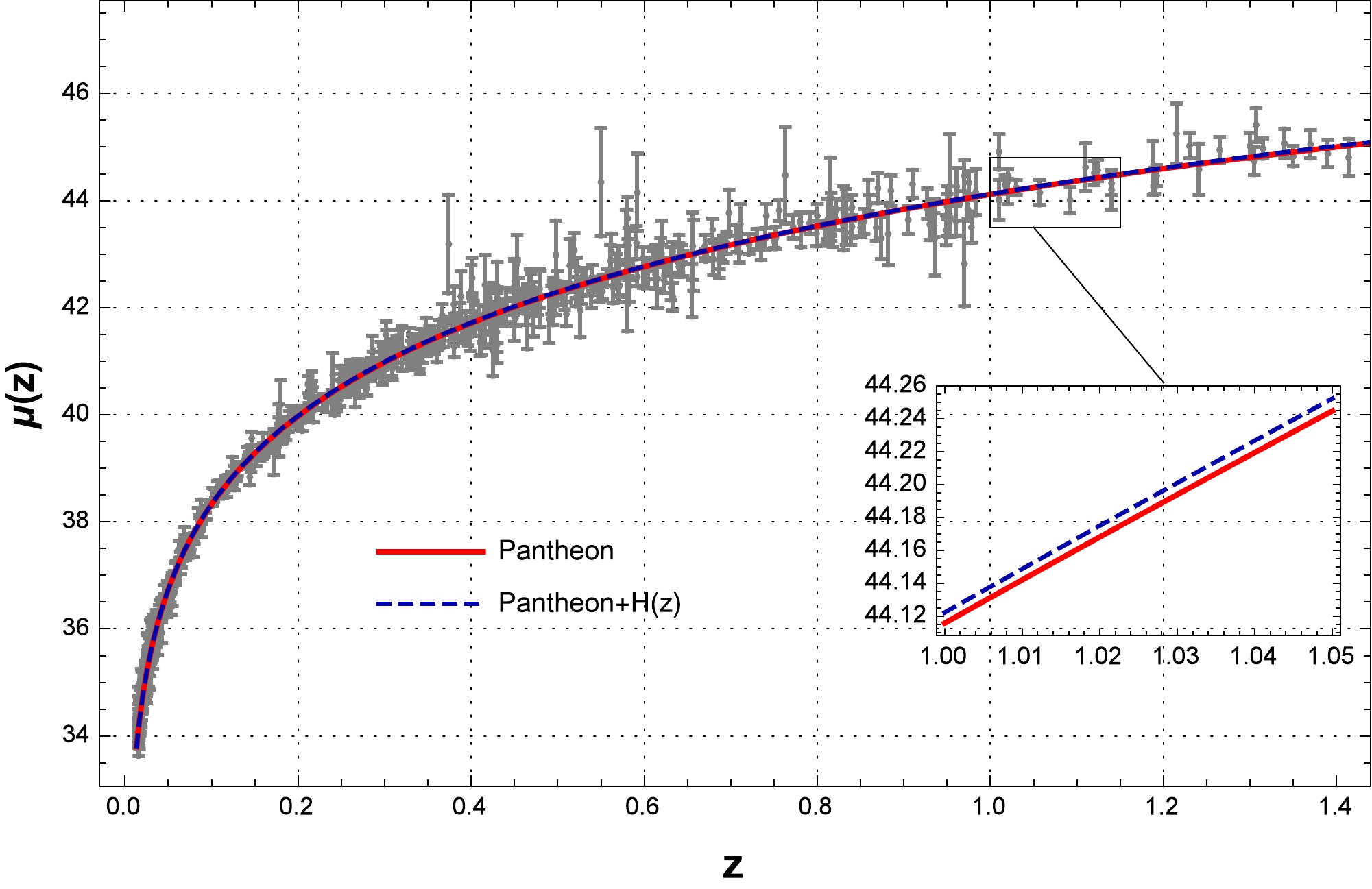
Figure 3. (color online) Supernovae data with the Pantheon sample (gray points) and the best-fit curves of the modulus distance μ as a function of the redshift z [Eq. (19)] for the parameterization of the DE model in an anisotropic universe. Each color represents a different dataset. The continuous (dashed) curves correspond to the Pantheon (Pantheon+H(z)) data.
The redshift evolution of the Hubble parameter
$ H(z) $ is reconstructed within the$ 1\sigma' $ confidence region in Fig. 4. The points with bars show the experimental data abstracted in Table 1. It is clear that our model is best-suited to the data when we perform a joint analysis of the two datasets. In all cases, we set$H_0=70\;\rm km/s/Mpc$ [46, 58]. As shown in this figure, the$ H(z) $ curve of the Pantheon data deviates from the$ 1\sigma' $ region at redshifts higher than$ z\sim0.9 $ .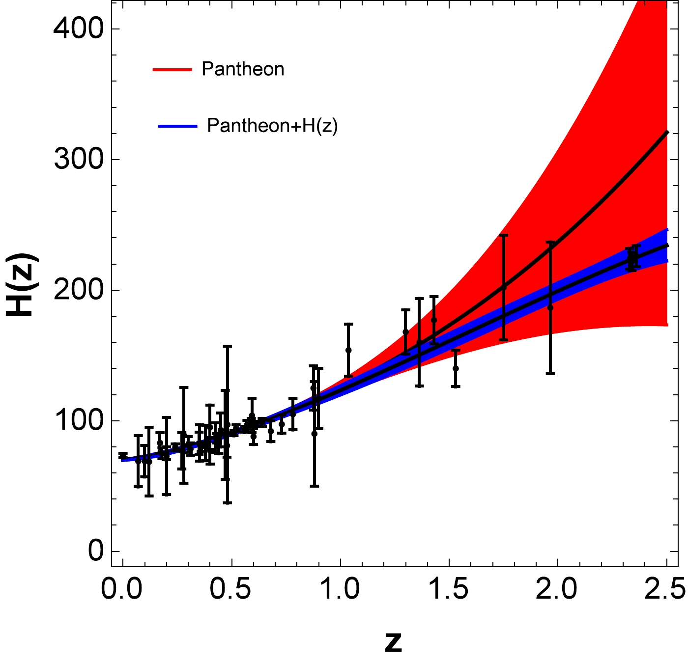
Figure 4. (color online) Reconstructed Hubble parameter
$ H(z) $ based on the best fit values of the cosmographic parameters for the parameterization of the DE model in an anisotropic universe. Table 1 summarizes the experimental data behind the points with bars. The red (blue) band shows the$ 1\sigma' $ confidence region using the Pantheon (Pantheon+H(z)) data.Having been constrained by the different observations, Fig. 5 shows the EoS for the parameterization of the DE model used at the
$ 68% $ % confidence level of the BI universe. The evolution in the Pantheon sample (red) moves close to$ \omega(z)=-1 $ . Nevertheless, as it approaches$ z=0 $ , the EoS approaches higher values toward$ \omega(z=0)= -1.016^{+0.305}_{-0.203} $ . By combining the Pantheon with H(z) data (blue), the EoS reaches a value of$ \omega(z=0)=-1.208\pm 0.17 $ , which is located in the phantom region. This scheme proposes a phantom crossing of the universe around$ z = 0.206 $ . In [67], the old SNIa data with the Gold dataset were used to reconstruct$ \omega(z) $ and exhibited a gentle preference for$ \omega(z) $ and the phantom evolution of the universe [68]. The WMAP7 measurements give$ \omega(z)=-1.1\pm0.14 $ [69], and an analysis of the Union2 SNIa dataset gives$ \omega(z)=-1.035\pm0.95 $ [70]. Therefore, the current observational data are still consistent with the phantom model.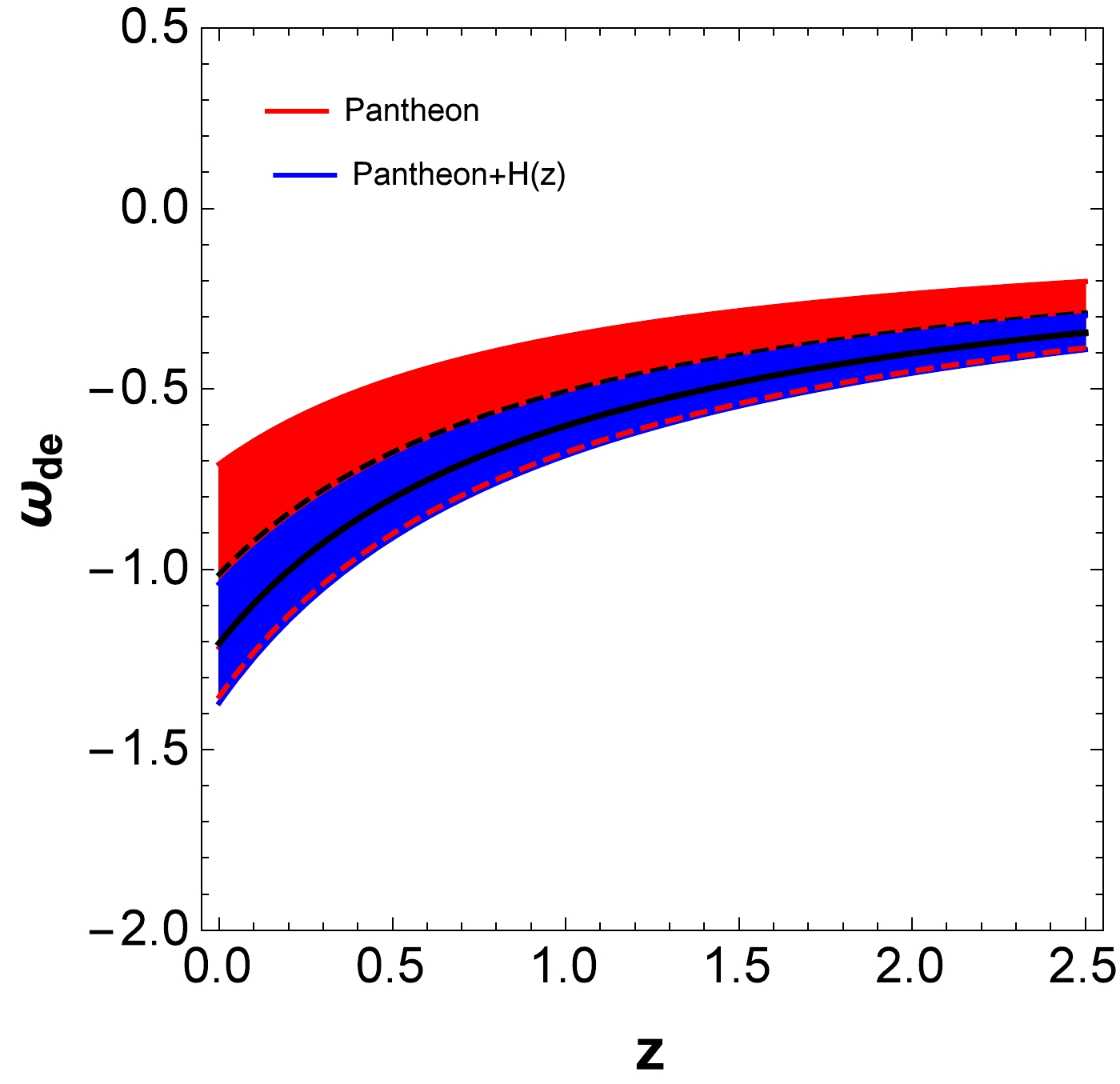
Figure 5. (color online) Posterior probability
$ Pr(\omega|z) $ of the DE EoS$ \omega=\omega_0/(1+z) $ against z. The red (blue) region represents the$1\sigma'(68\%)$ confidence contour level using the Pantheon (Pantheon+H(z)) data.Figure 6 shows a similar graph for the posterior probability of the deceleration parameter
$ q(z) $ at the$ 1\sigma' $ confidence level. We can see a flip in the signature of the deceleration parameter, which exhibits a transition from the decelerated phase to an accelerated phase; therefore, it is essential for the formation of a not hindered structure of the universe. In the parameterization DE model approach, the best suited value of the deceleration parameter within the$ 1\sigma' $ confidence level is$ q_0=-0.73\pm0.13 $ and$ q_0=-0.80\pm0.08 $ when considering the Pantheon and Pantheon+H(z) samples, respectively. We find that adding H(z) to the Pantheon data leads to a smaller value of the deceleration parameter compared to that of the solely Pantheon sample. Recently, Shrivastava [52] obtained an empirical value of$ q_0 $ as$ -0.61^{+0.03}_{-0.02} $ with Pantheon+H(z) in FRW cosmology. Furthermore, Ref. [71] considered the parameterization of the deceleration parameter in modified symmetric teleparallel gravity ($ f(Q) $ ) and obtained the current deceleration parameter value$ q_0=-0.832\pm0.091 $ , which is close to our result.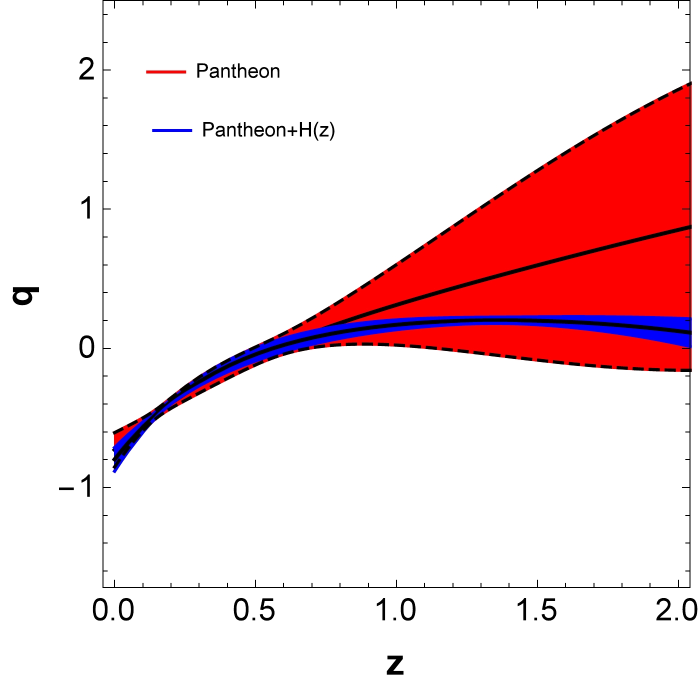
Figure 6. (color online) Posterior probability
$ Pr(q|z) $ of the deceleration parameter$ q(z) $ against z. The red (blue) region represents the$1\sigma'(68\%)$ confidence contour level using the Pantheon (Pantheon+H(z)) data.Finally, we consider the isotropize model. The measure of anisotropy is described by
${\sigma}/{H}$ , expressing the magnitude of the space-time shear per average expansion rate. The criterion of late-time isotropization in an expanding universe ($ H>0 $ ) is the vanishing of the shear$ \sigma\rightarrow 0 $ , or alternatively, we can use the condition${\sigma}/{H}\rightarrow 0$ at$ t\rightarrow \infty $ . Evolution of the anisotropy parameter${\sigma}/{H}$ with respect to the redshift z for the parameterization of the DE model with the Pantheon and Pantheon+ H(z) datasets is presented in Fig. 7. However, as shown in Fig. 7, the anisotropy is a non-zero value at the present time,$ z=0 $ , although it is approaching zero, i.e., the anisotropy will be very low after inflation. Then, at the end of inflation,$ \mathcal{O}(10^{-6}) $ , which is closer to the bound obtained by [72].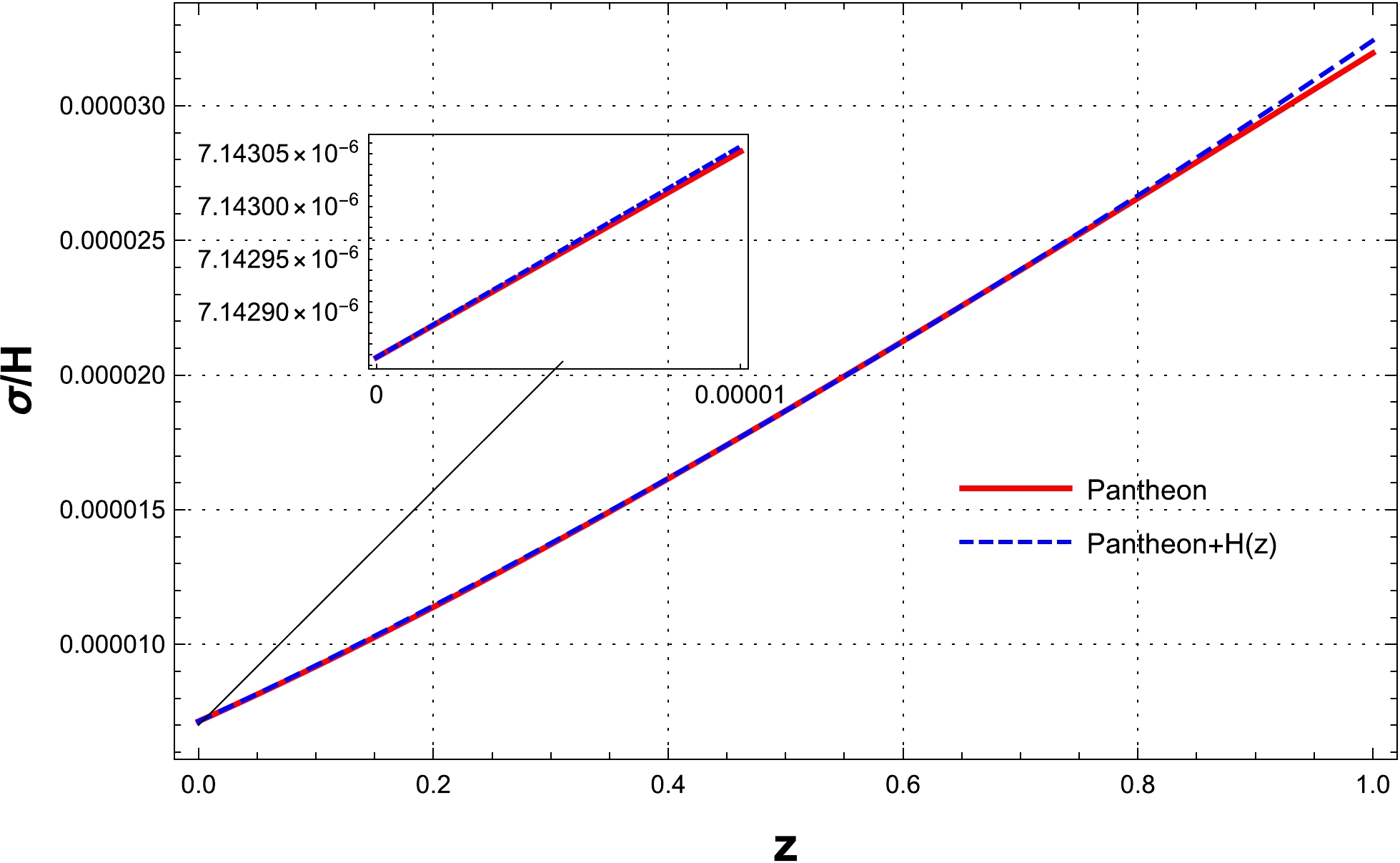
Figure 7. (color online) Plot of the evolution of the anisotropy parameter versus redshift for the parameterization of the DE model in an anisotropic universe. The figure is obtained using the best-fit values for the Pantheon and Pantheon+H(z) datasets presented in Table 2.
-
In this study, Pantheon and H(z) datasets are used to construct observational constraints on the parameterization of DE (
$ \omega(z)=\omega_0/(1+z) $ ) in the scope of an anisotropic BI universe. We perform a perfect solution to Einstein's field equations for the parameterization of the DE case in BI space-time. Figures 1 and 2, in the circumstances under the cosmography approach, demonstrate how the best-fit values of the confidence of the cosmographic parameters for different combinations of data samples indicate regions up to$ 2\sigma' $ uncertainties. Table 2 summarizes the major findings of the statistical analysis. Alongside the parameterization DE case, we use one prior for$ H_0 $ from Refs. [46, 58]. We also check the statistical performance of the parameterization model studied in this paper by computing the$\chi^2_{\min}$ ,$\chi^2_{\rm red}$ , and AIC estimators (see Table 3). We realize that with the evolving parameterization of DE, the Pantheon+H(z) sample seems to be favored over the Pantheon sample. The Hubble parameter is reconstructed using the best fit value of the cosmographic parameters for DE parameterization. For the parameterization of DE, we notice that the evolution of the reconstructed H(z) in the Pantheon sample in comparison with different data sample combinations has the maximum deviation from the confidence region. By incorporating different combinations of data samples, our results show that the best fit value of the deceleration parameter$ q_0 $ changes in the range$ -0.88 $ to$ -0.72 $ and the EoS parameter$ \omega(z=0) $ changes in the range$ -1.25 $ to$ -1.16 $ . Based on the results of Figs. 5 and 6, when we use the Pantheon sample alone, the deceleration parameter$ q_0 $ and EoS parameter$ \omega(z=0) $ have the largest values, whereas adding the H(z) data sample to Pantheon leads to smaller values for$ q_0 $ and$ \omega(z=0) $ . We also obtain a general condition for the phantom barrier crossing of the parameterization of the DE model in the BI universe. We study the evolution of$\dfrac{\sigma}{H}$ , as shown in Fig. 7. We find that the fraction of the anisotropy of the universe to shear scalar can increase to$ \mathcal{O}(10^{-6}) $ at the present time. Finally, we deduce that the current Pantheon and H(z) data with effects of anisotropy effectively constrain free values. Additionally, our model confirms recent observations. -
No data were used for the research described in the article.
Phantom cosmologies from the simplest parameterization of the DE model using observational data in a BI type universe
- Received Date: 2023-06-21
- Available Online: 2023-11-15
Abstract: To scrutinize the nature of dark energy, many equations of state have been proposed. In this context, we examine the simplest parameterization of the equation of state parameter of dark energy in an anisotropic Bianchi type I universe compared with the ΛCDM model. Using different combinations of data samples, including Pantheon and Pantheon + H(z), alongside applying the minimization of the


 DownLoad: