


 Abstract
 HTML
HTML Reference
 Related
 PDF
PDF


-
The consequences of self-gravitating objects are a fascinating area of study in general relativity (GR). It is impossible for anything, even light, to escape the catastrophic thermodynamic grip of a black hole (BH) because it is so massive and governed by its own gravity. The unusual thermodynamic features of BHs make them an ideal platform for gravitational physics experiments. BH dynamics laws were discovered by Bardeen, Carter, and Hawking [1].
After the breakthrough of Hawking and Page [2], interest in BH thermodynamics, for example, phase transitions, began to grow. Similarities exist between the phase changes of van der Waals fluids and charged Reissner-Nordstrom (RN) BHs. Davies [3] investigated Kerr-Newman BH phase space and developed the thermodynamic theory of BHs. Biswas and Chakraborty [4] found that depending on the value of r, Horava Lifshitz gravity BHs can be either stable or unstable. Kubiznak and Mann [5] compared the liquid-gas composition of fluids during phase changes in charged AdS BHs. The thermal characteristics of regular BHs and phase transitions were reviewed and initiated by Tharanath et al. [6] B5), who expressed that regular BHs experience a second-order phase transition. The gauge duality representation in thermal field theory [7] is interesting because of the holographic link between gravity systems and conformal field theory (AdS/CFT duality), which makes anti-de Sitter space-time intriguing.
Classical and quantum gravitational effects are easy to identify because BH mechanics are equivalent to thermodynamics. Owing to the resemblance between BH physics and classical thermodynamics, BH mass responds to enthalpy by converting internal energy [8], entropy (which is proportional to the horizon radius, temperature, and surface gravity), and the cosmological constant (which is equivalent to pressure and volume as its thermodynamically conjugate variables). Because of this correspondence, any other object of the same volume must have maximum BH entropy. Otherwise, the proposed relation would be violated.
In this situation, the BH and thermal radiation are not in thermal equilibrium. By examining the quantum fluctuation, which is linked with BH evaporation, this enigma can be resolved. At the quantum level, the BH ejects subatomic particles, which are known as Hawking radiation, and provides knowledge about the concepts of thermal fluctuation, the holographic principle, and BH geometry. In this way, Bekenstein proposed the area-entropy relation, for which correction is required with this prominent association in the concepts of the holographic principle and the effect of thermal fluctuations [9]. From thermal fluctuations, the area-entropy relationship must be corrected with some logarithmic term. Fluctuation is a process that occurs due to statistical perturbations in compact objects, which has a remarkable impact on the structure of BHs. It has been observed that the area of a BH decreases due to Hawking radiation; therefore, its temperature increases. Pourhassan and Faizal [10] found that thermal fluctuations correct BH entropy via the logarithmic correction term and are significant for small BHs. In [11], Faizal and Khalil revealed the effect of logarithmic corrections on the thermodynamics of three BHs and found that these BHs produced remnants in all situations. Okcuet et al. [12] and Zhang [13] analyzed the effects of first-order correction terms on RN-AdS and Kerr-Newman-AdS BH entropy. The implications of thermal fluctuations on non-minimal regular BHs in the presence of cosmological constants were investigated by Jawad and Shahzad [14], who noted that with large values of the cosmological constant, BHs are stable in both local and global phases. Pradhan [15] investigated the thermodynamics and thermal fluctuations of charged accelerating BHs. Quasi-normal modes (QNMs) are the modes of energy that describe the perturbation of a field and give critical information about the structure of compact objects such as BHs. This phenomenon classifies BHs with other stellar structures. Vishveshwara [16] was the first to take a revolutionary step to demonstrate the analytical representation of QNMs from wave functions for Schwarzschild BHs. After studying the association between the second-order phase transition of RN-BHs and QNMs, Jing and Pan [17] stated that the frequency of QNMs takes a spiral shape, having an oscillatory function of charge. For charged Kaliza-Klein BHs of QNM perturbation, He et al. [18], examined the relationship between QNMs and phase transition. Meanwhile, examining various features of BH perturbation, Konoplya and Zhidenko [19] recognized the decoupling of various components in the perturbed equation and gravitational stability.
The foundation of BH perturbations was the innovative work of Regge, Wheeler, and Zerilli [20] and [21]. Leaver [22] expressed an analytic illustration of the QNM wave-functions of both static and moving BHs. To consider the massless scalar fields of QNMs as well as absorption, Breton et al. [23] used the Wentzel-Kramers-Brillouin (WKB) approach, including null geodesics. Jusufi and Ovgun [24] described QNMs and the stability for BHs minimally linked to a cloud of strings. Churilova [25] added corrections to Einstein theory due to deviations and developed interpretive QNMs of BHs. He also obtained an empirical correlation for analyzing eikonal QNMs in Schwarzschild geometry. The QNMs and the solution with cosmic string of the Klein-Gordon equation in Born-Infeld (BI) dilaton space-time were measured by Sakalli et al. [26]. Wei and Liu [27] found that QNMs could be made from null geodesics using the angular velocity and Lyapunov exponent of the photon sphere and concluded that QNMs for RN-BHs have an analytical correspondence in the eikonal limit. More recently, Abbas and Ali [28] analyzed the effects of thermal fluctuations, QNMs, and phase transition on a charged RN-BH surrounded by perfect fluid dark matter (PFDM) and revealed that BHs with large radii are more stable under the influence of logarithmic correction.
It is worth noting that phase space for charged-AdS BHs must be studied in the context of nonlinear electrodynamics (NLED). The solution of the Einstein field equations connected to the NLED of BI is given in [29], for BI BHs. BI vacuum polarization is a parameter of the BI thermodynamic conjugate variable. This indicates that the first law of thermodynamics and the Smarr relation are consistent. Motivated by such a progressive approach suggested by Euler and Heisenberg [30], we investigate the thermodynamics of the quantum electrodynamics-based BH solution coupled with NLED. To better characterize the electromagnetic field, Euler and Heisenberg came up with a novel approach that was inspired by Dirac's positron theory. They were able to determine the effective Lagrangian electromagnetic field density by modifying Maxwell's equation while it was being solved in a vacuum, and such an effective Lagrangian density has a higher order term than the NLED field [31]. For an electric field, the effects of NLED that result in a Schwinger field with an order (
$ E_{c} 10^{18} $ ) V/m are currently being empirically detected [32]. Euler-Heisenberg (EH) theory has been well established, and it has been shown that these effects are present. Kruglov obtained a charged BH in the field of NLED by applying an EH-based model with two parameters [33]. It is important to remember that Kruglov developed the effective geometry of NLED and showed how big the shadows of three static BHs were [34].EH theory is a better traditional approximation of quantum electrodynamics when the field is strong. Maxwell's theory suggests a way of measuring the EH effect. In EH theory, there are some important physical properties that lead the EH Lagrangian to the Ricci scalar through the volume to find the BH solution. Electrically charged BHs were suggested in [35]. In [36], researchers looked at how charged particles moved around AdS EH BHs. In [37−39], the EH Lagrangian and modified gravity theories were introduced. In [40], researchers looked into the shadows of EH BHs. Schwinger [41] renormalized the field strength and charge of the modified Lagrange function for constant fields. In EH, Yajima and Tamaki [42] constructed BH solutions that were spherically symmetric and static. Runi et al. [43] came up with EH theory and looked into the solutions of non-rotating BHs with electric and magnetic charges in spherical geometry. They did this by using the EH effective Lagrangian of one-loop non-perturbative quantum electrodynamics contributions. Magos and Breton [44] demonstrated the consistency of the Smarr formula with the first law of BH thermodynamics by including the cosmological constant in their solution.
In this study, we examine EH-BHs from a thermodynamic perspective in extended phase space, where the cosmological constant is the dynamical pressure. Recently, in [45], the authors investigated the phase transition via high-order quantum correction and explored the EH-AdS BH solution and its critical exponents. They [46] demonstrated the geometric optics of EH BHs under the influence of different accretion flows. The study of the first-order phase transition of EH-AdS BHs on the basis of the free energy landscape and probability distribution of the system has been discussed in [47]. Karakasis et al. [48] studied EH theory in the presence of a self-interacting scalar field minimally coupled to gravity and explored second-order phase transitions and their stability.
The objective of this paper is to demonstrate the thermodynamic quantities with the correction term of entropy through thermal fluctuation with simple logarithmic corrections for an EH-AdS BH with NLED. Furthermore, we examine the QNMs and phase transition of the EH-AdS BH with NLED. The paper is arranged as follows. In Sec. II, we review the solution of the EH-AdS BH in NLED. In Sec. III, we represent the corrected quantities of thermodynamics via the thermal fluctuation. We establish a relation between null geodesics and QNMs in Sec. IV, discuss the phase transition in Sec. V, and summarize our findings in Sec. VI.
-
In this section, we briefly review EH-NLED field theory, which is coupled to gravity and the cosmological constant. The action of GR is associated with NLED, which is given by [49−51]
$ \begin{equation} S=\frac{1}{4 \pi}\int_{M^{4}} {\rm d}^{4}x\sqrt{-g}\Bigg(\frac{1}{4}(R-2\Lambda)-\mathcal{L}(A,G)\Bigg), \end{equation} $

(1) where g is the determinant of the given metric tensor, and
$ \mathcal{L}(A,G) $ is the NLED Lagrangian density, which relies on the electromagnetic invariants$ \begin{equation} A=\frac{1}{4}A_{\mu \nu} A^{\mu \nu},\,\,\,\ {\rm and} \,\,\,\,\,\ G=\frac{1}{4}A_{\mu \nu}\, ^*A^{\mu \nu}, \end{equation} $

(2) where
$ A_{\mu \nu} $ is the electromagnetic field strength, and$ \, ^*A^{\mu \nu}=\varepsilon_{\mu \nu \varphi\psi}A^{\varphi\psi}/2 \sqrt{-g} $ is its dual. The antisymmetric tensor$ \varepsilon_{\mu \nu \varphi\psi} $ satisfies$ \varepsilon_{\mu \nu \varphi\psi} \varepsilon^{\mu \nu \varphi\psi}=-4! $ .The Lagrangian density for EH-NLED [30] is of the form
$ \begin{equation} \mathcal{L}(A,G)=-A+\frac{\alpha}{2}A^{2}+\frac{7\alpha}{8}G^{2}, \end{equation} $

(3) where
$ \alpha=\dfrac{8\hat{\alpha}^{2}}{45 m^{4}} $ is the EH parameter that governs the intensity of the NLED endowment, and m and α are the mass of an electron and the structural constant, respectively. If$ \alpha=0 $ , we regain the Maxwell electrodynamics$ \mathcal{L}(A)=-A. $ Here, we deal with two systems regarding NLED, the A system in terms of the electrodynamic field tensor
$ A^{\mu\nu} $ , and the J system with the tensor$ J_{\mu\nu} $ as the essential field, which is of the form$ \begin{equation} J_{\mu\nu}=-(\mathcal{L}_{A} A_{\mu\nu}+\, ^*A_{\mu\nu}\mathcal{L}_{G}), \end{equation} $

(4) where
$\mathcal{L}_{A}=\dfrac{{\rm d}\mathcal{L}}{{\rm d}A}$ and$\mathcal{L}_{G}=\dfrac{{\rm d}\mathcal{L}}{{\rm d}G}$ .From EH theory,
$ J_{\mu\nu} $ is defined as$ \begin{equation} J_{\mu\nu}=(1-\alpha A) A_{\mu\nu}-\, ^*A_{\mu \nu }\frac{7 \alpha}{4}G. \end{equation} $

(5) Eq. (5) establishes a relationship between the intensity and electric field in EH-NLED.
There are two invariants, J and O, coupled to the framework J, defined as
$ \begin{equation} J= \frac{-1}{4}J_{\mu\nu}J^{\mu\nu},\,\,\,\,\,\,\,\ O=\frac{-1}{4}J_{\mu\nu}\, ^*J^{\mu \nu }, \end{equation} $

(6) with
$ \begin{equation} \, ^*J_{\mu\nu}= \frac{1}{2 \sqrt{-g}}\varepsilon_{\mu\nu\varphi\psi}J^{\varphi\psi}. \end{equation} $

(7) The Hamiltonian is defined by the Legendre transformation of
$ \mathcal{L} $ as follows:$ \begin{equation} \mathcal{H}(J,O)=\frac{-1}{2}J^{\mu\nu}A_{\mu\nu}-\mathcal{L}. \end{equation} $

(8) By neglecting the second and higher terms in α, the Hamiltonian for EH theory takes the form
$ \begin{equation} \mathcal{H}(J,O)=J-\frac{\alpha}{2}J^{2}-\frac{7\alpha}{8}O^{2}. \end{equation} $

(9) The corresponding field equations [50] are
$ \begin{equation} J^{\mu\nu},\mu=0, \,\,\,\,\,\ G_{\mu\nu}+\Lambda g_{\mu\nu}=8\pi T_{\mu\nu}. \end{equation} $

(10) The energy-momentum tensor takes the form
$ \begin{equation} T_{\mu\nu}=\frac{1}{4\pi}\Bigg((-J\alpha+1)J^{\gamma}_{\mu}J_{\nu\gamma}+g_{\mu\nu}\Bigg(J-\frac{3}{2}\alpha J^{2}-\frac{7\alpha}{8}O^{2}\Bigg)\Bigg). \end{equation} $

(11) The field equation Eq. (11) is solved with the cosmological constant. The metric is given by
$ \begin{equation} {\rm d}s^{2}= -N(r){\rm d}t^{2}+ \frac{1}{N(r)}{\rm d}r^{2}+ r^{2}({\rm d}r^{2}+\sin^{2}\theta {\rm d}\phi^{2}), \end{equation} $

(12) and concerning the electromagnetic field, along with charge Q, the non-vanishing components are
$ \begin{equation} J_{\mu\nu}=\frac{Q^{2}}{r^{2}}\delta^{1}_{[\mu}\delta^{2}_{\nu]}\ , \end{equation} $

(13) and hence the electromagnetic invariants are
$ \begin{equation} J_{\mu\nu}=\frac{Q^{2}}{2r^{4}}, \,\,\,\,\,\ O=0. \end{equation} $

(14) Inserting these into the (1,1) components of Eq. (10), we obtain
$ \begin{equation} \frac{{\rm d}m}{{\rm d}r}=\frac{Q^{2}}{2r^{2}}-\frac{\alpha Q^{4}}{8r^{6}}+\frac{\Lambda r^{2}}{2}. \end{equation} $

(15) Solving the above equation, with the electric charge, the respective metric is of the form
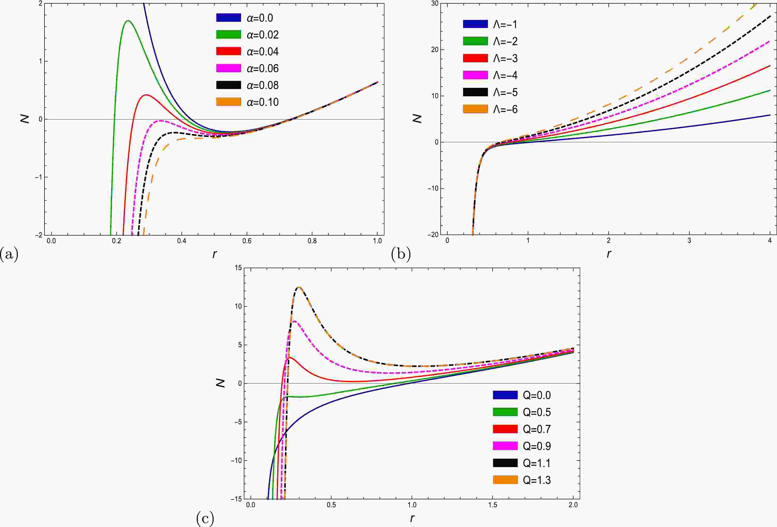
$ \begin{equation} N(r)= 1- \frac{2m}{r}+ \frac{Q^{2}}{r^{2}}-\frac{\Lambda r^{2}}{3}-\frac{\alpha Q^{4}}{20r^{6}}, \end{equation} $

(16) where m, Q, α, and Λ are the geometrical mass of the BH, electric charge, EH parameter, and cosmological constant, respectively. Here, Eq. (16) represents an EH-AdS BH; for
$ \Lambda=0 $ , it corresponds to an EH-BH [46]. If$ \alpha\rightarrow0 $ and$ \Lambda=0 $ , the above equation reduces to an RN-BH [12], and if$ Q=0 $ , it becomes an AdS-Schwarzschild BH [2].Figure 1 provides an interpretation of the horizon radius with a variation in three parameters.
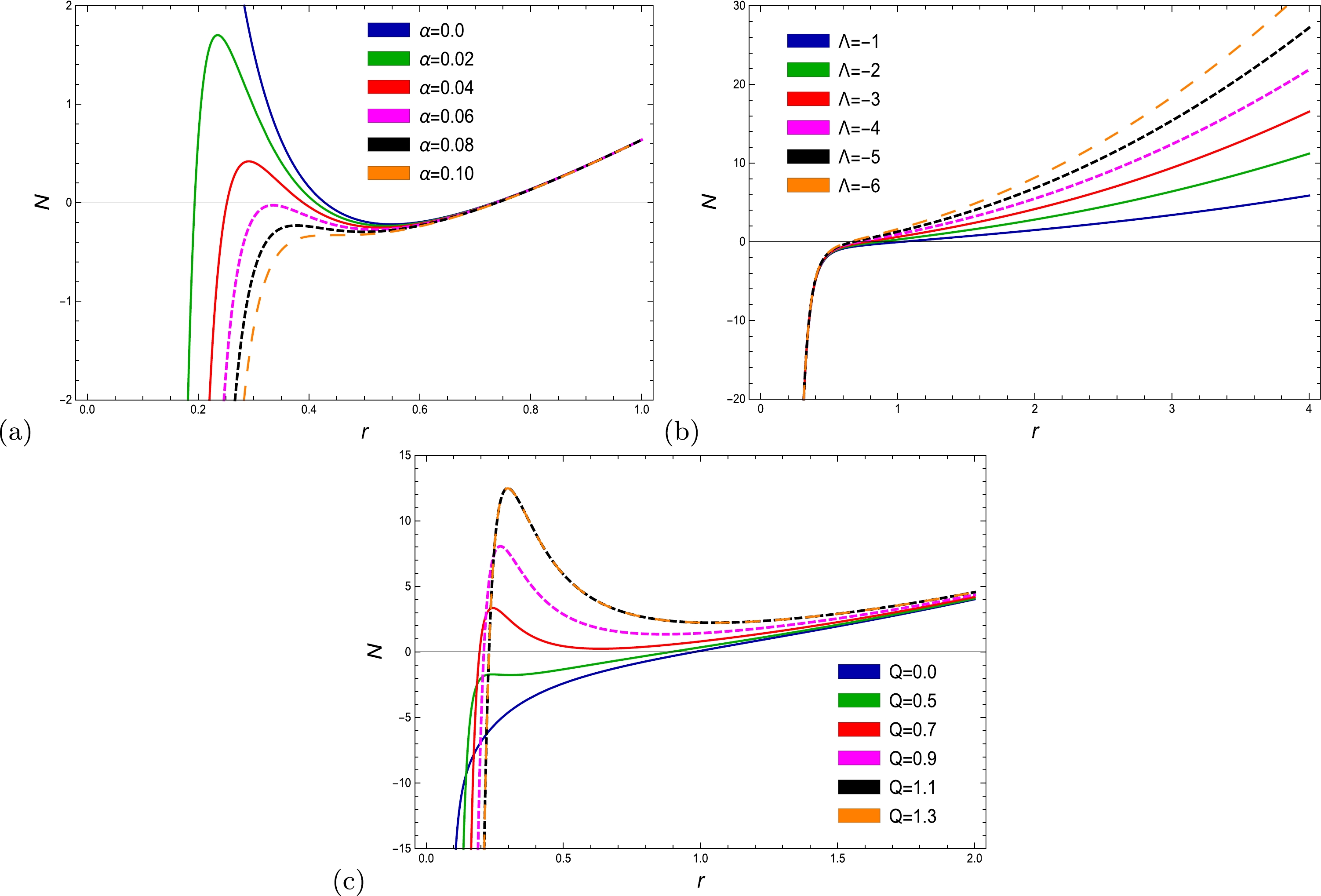
Figure 1. (color online) Graph of the metric function versus horizon radius r with altered values of all three parameters α, Λ, and Q along with
$ M = 1 $ . (a)$ \Lambda = -3 $ ,$ Q = 0.8 $ , (b)$ Q = 0.8 $ ,$ \alpha = 1 $ , and (c)$ \alpha = 0.02 $ ,$ \Lambda = -3 $ . -
In the context of thermodynamics, we discuss the thermodynamical potentials of EH-AdS BHs with NLED. Moreover, we concentrate on the entropy correction of EH-AdS BHs with NLED to drive the corrected thermodynamic quantities. These updated quantities include entropy, Helmholtz free energy, total corrected mass, pressure, Gibbs free energy, enthalpy, and specific heat. The BH entropy can be written as follows:
$ \begin{equation} S_0= \frac{A}{4}=\pi r_+^2, \end{equation} $

(17) Entropy is relevant to the BH event horizon, which affects the thermal properties. The second law of thermodynamics suggests that BH entropy must be higher than any comparable volume. The corrected entropy expression is obtained using the partition function [15] as follows:
$ \begin{equation} Z(\beta)= \int^{\infty}_{0} {\rm e}^{-\beta E}\rho(E){\rm d}E, \end{equation} $

(18) where E and
$ \rho(E) $ denote the average energy and quantum density, respectively. The inverse Laplace transformation of the partition function gives the quantum density in the following form:$ \begin{equation} \rho(E)= \frac{1}{2\pi i}\int^{i \infty +\beta_{0}}_{-i \infty +\beta_{0}} {\rm e}^{-\beta E}Z(\beta){\rm d}\beta = \frac{1}{2\pi i}\int^{i \infty +\beta_{0}}_{-i \infty +\beta_{0}}{\rm e}^{S(\beta)}{\rm d}\beta, \end{equation} $

(19) where
$ \beta>0 $ , and$ S(\beta)=\ln Z(\beta)+\beta E $ is the corrected entropy, which is dependent on Hawking temperature. Via Taylor's expansion, we get$ \begin{equation} S(\beta)=S_{0}+\frac{1}{2} (\beta-\beta_{0})^{2}\frac{\partial^{2}S(\beta)}{\partial\beta_{2}}\Big|_{\beta=\beta_{0}}. \end{equation} $

(20) The corrected entropy provides the relations
$ \dfrac{\partial S}{\partial\beta}=0 $ and$ \dfrac{\partial^{2} S}{\partial\beta^{2}}>0 $ at the point of equilibrium. Now, using Eq. (18) in Eq. (17) gives us$ \begin{equation} \rho(E)= \frac{{e}^{S}}{2\pi i} \int {\rm e}(^{\frac{1}{2}(\beta-\beta_{0})^{2}\frac{\partial^{2}S(\beta)}{\partial\beta^{2}}}) {\rm d} \beta, \end{equation} $

(21) which is the same as given in . The simplified form of the above equation is
$ \begin{equation} \rho(E)= \frac{1}{\sqrt{2\pi}}{\rm exp}(S)\Bigg(\Bigg(\frac{\partial^{2} S}{\partial\beta^{2}}\Bigg)\Big|_{\beta=\beta_{0}}\Bigg)^{\frac{-1}{2}}. \end{equation} $

(22) Therefore, after simplification, we get
$ \begin{equation} S=S_{0}-\frac{1}{2}\ln(S_{0}T^{2})+\frac{\chi}{S_{0}}. \end{equation} $

(23) The corrected terms of the BH entropy can be improved by substituting the factor
$ \frac{1}{2} $ for a more general parameter called$ eta $ . As a result, the corrected entropy can be rewritten as [10−12, 14, 28, 51]$ \begin{equation} S=S_{0}-\eta\ln(S_{0}T^{2})+\frac{\chi}{S_{0}}, \end{equation} $

(24) where χ is the correction parameter for the higher order correction. The different values of the parameter of η and χ have following consequences:
I- When χ,
$ \eta \rightarrow 0 $ , it provides the entropy of the BH without corrections.II- For η,
$ \chi \rightarrow 1 $ , these are the correction terms of a higher order.III- For
$ \chi \rightarrow 1 $ ,$ \eta \rightarrow 0 $ , it allows a second-order correction.IV- As
$ \chi \rightarrow 0 $ ,$ \eta \neq 0 $ , we usually obtain a simple logarithmic correction.Throughout this paper, we assume the simple logarithmic corrections case (
$ \chi \rightarrow 0 $ ,$ \eta \neq 0 $ ) to determine the thermodynamical properties. It is worth noting that the logarithmic terms in Eq. (17) correct the BH entropy. -
We can obtain the BH geometrical mass using the horizon radius by setting
$ N(r_{+})=0 $ , that is,$ \begin{equation} m=\frac{1}{2} r_+ \left(\frac{r_+^2}{l^2}-\frac{\alpha Q^4}{20 r_+^6}+\frac{Q^2}{r_+^2}+1\right). \end{equation} $

(25) The total mass of the BH is obtained using the definition from Abbott and Deser [52−53],
$ \begin{equation} M=\frac{m}{8}=\frac{1}{8}\left(\frac{1}{2} r_+ \left(\frac{r_+^2}{l^2}-\frac{\alpha Q^4}{20 r_+^6}+\frac{Q^2}{r_+^2}+1\right)\right). \end{equation} $

(26) The Hawking temperature is equivalent to the surface gravity κ, which is defined by
$ T=\frac{\kappa}{2 \pi}=\frac{N'}{4 \pi}, $

which further simplifies to
$ \begin{equation} T=\Big(\frac{3r_+}{4\pi l^2}-\frac{Q^2}{4\pi r_+^3}+\frac{\alpha}{4\pi r_+^2}+\frac{1}{4\pi r_+}\Big). \end{equation} $

(27) The thermodynamical stability of the Einstein EH (EEH)-Ads BH can be investigated via the specific heat, which is given by
$ C=T\frac{\partial S_{0}}{\partial T}, $

$ \begin{equation} C=\frac{2 \pi r_+^2 \left(l^2 \left(\alpha Q^4-4 Q^2 r_+^4+4 r_+^6\right)+12 r_+^8\right)}{l^2 \left(-7 \alpha Q^4+12 Q^2 r_+^4-4 r_+^6\right)+12 r_+^8}. \end{equation} $

(28) The diagrams of Hawking temperature and heat capacity against the horizon radius with altered electric charge values of the EEH-AdS BH are presented in Figs. 2 and 3 . By vanishing
$ \alpha=0 $ , it reduces to the RN-AdS BH [5], and by removing both parameters$ \alpha=0 $ ,$ Q=0 $ , it is the Schwarzschild-AdS BH [2]. Now, we employ the corrected entropy and Hawking temperature to study the thermodynamic equation of state. Substituting Eqs. (27) and (17) into Eq. (24), the corrected entropy becomes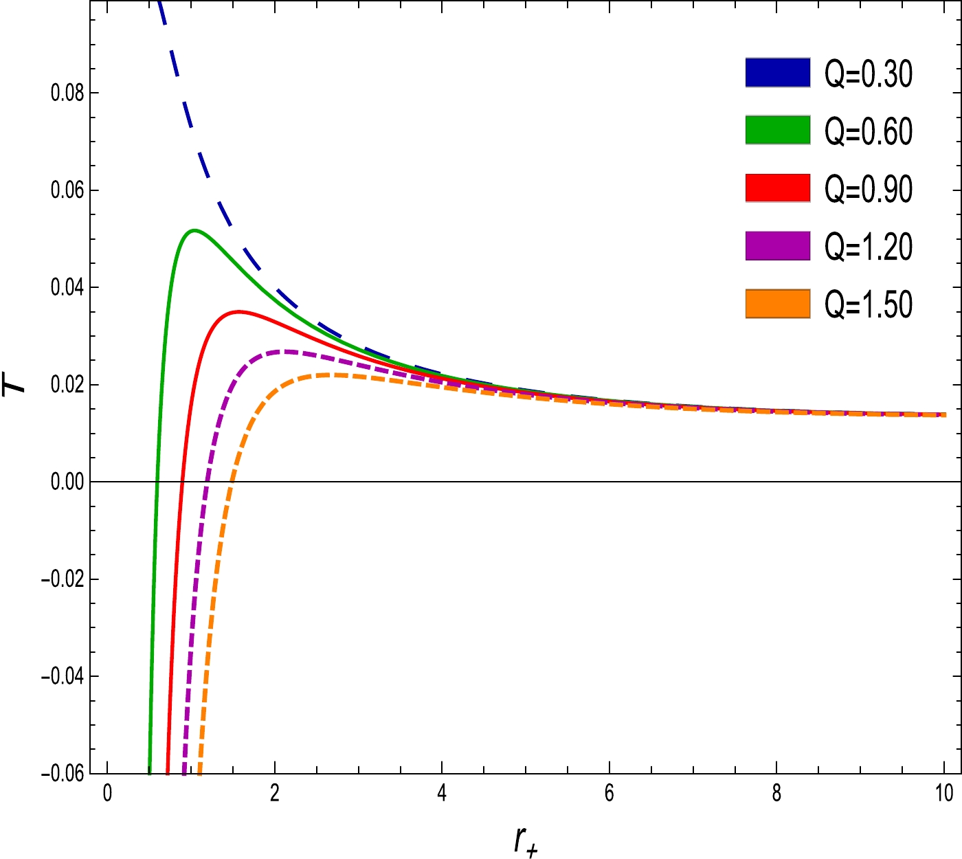
Figure 2. (color online) Graph of T as a function of
$ r_{+} $ for$ \alpha=0.02 $ and$ l=20 $ .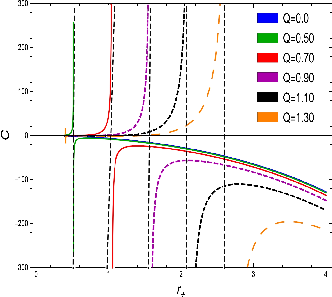
Figure 3. (color online) Graph of C as a function of
$ r_{+} $ for$ \alpha=0.02 $ and$ l=20 $ .$ \begin{aligned}[b] S=&\eta \log \left(256 \pi l^4 r_+^{12}\right)-2 \eta \log \Big(l^2 \left(\alpha Q^4-4 Q^2 r_+^4+4 r_+^6\right)\\&+12 r_+^8\Big)+\pi r_+^2. \end{aligned} $

(29) In Fig. 4, the graphical profile of corrected entropy vs. horizon radius
$ r_{+} $ is displayed with different parametric values of Q, η, and α. It is observed that the corrected entropy satisfies the second law of thermodynamics because it remains positive and stable for all the given parameters. In Refs. [54−65], entropy modifications were observed for various BHs. We found that the considered BH became unstable due to the presence of thermal fluctuation. Owing to the positive correction parameter, we found that the corrected entropy increased and remained stable, as investigated in [54]. This means that the effects of thermal fluctuation keep the entropy function positive. Based on the results presented in [55], we determine that the corrected entropy is not well suited for BHs with large horizon radii and is not significantly affected by small thermal fluctuations. Plot (a) shows that the entropy function has a positive value as the horizon radius increases and decreases only for small radii. It should be noted that as the charge parameter increases, the corrected entropy function increases. Plot (b) indicates that with an increase in the coupling and corrected parameters, the entropy becomes more stable for large-radius BHs compared to small-radius BHs. Moreover, plot (b) explains the corrected entropy when the coupling parameters$ \alpha=0 $ and$ \alpha\neq0 $ . Graphically, it reveals the behavior of the corrected entropy for RN-AdS BHs [12] in the absence of α, and for altered values of the coupling parameter, it demonstrates the corrected entropy of EH-AdS BHs. Similarly, plot (c) shows the uncorrected entropy when $ \eta=0 $ and the corrected entropy when$ \eta\neq0 $ and presents the increasing behavior for corrected and usual entropy. Moreover, the corrected entropy becomes greater than usual entropy, and with an increase in the correction parameter, entropy becomes maximum. As a result, the effect of thermal fluctuation is limited to a small radius and remains stable for a large radius. In comparison with our recent work [28], the corrected entropy of BHs is consistently greater than the usual entropy owing to thermal fluctuations. This leads to the conclusion that the equilibrium state of BHs becomes unstable. Based on the provided physical description, it is evident that when the coupling parameter of PFDM, denoted as α, is set to zero, the corrected entropy of RN-BHs is restored.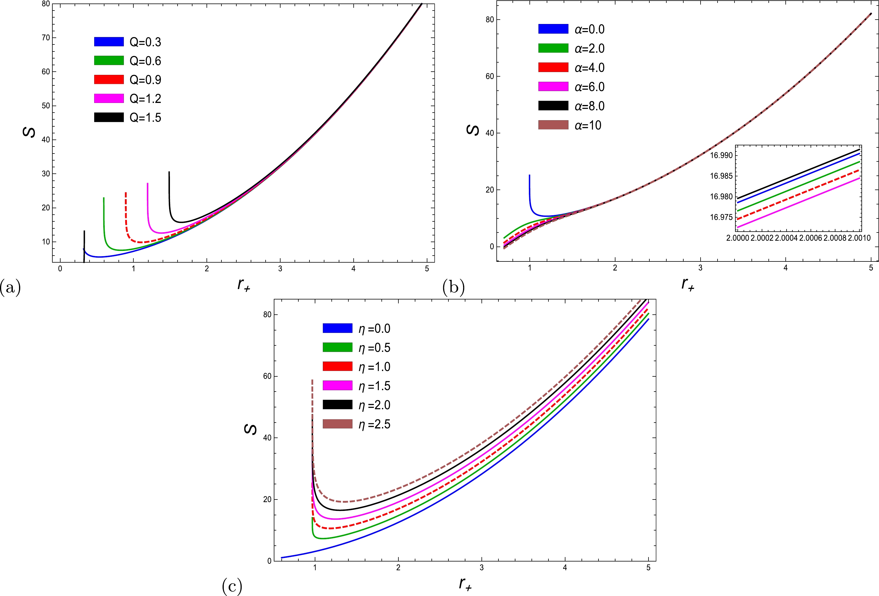
Figure 4. (color online) Corrected entropy as a function of
$ r_{+} $ with$ l = 20 $ and (a)$ \alpha = 0.02 $ ,$ \eta = 1 $ , (b)$ \alpha = 0.2 $ ,$ Q = 1 $ , and (c)$ Q = 1 $ ,$ \eta = 1 $ .In the current study, the corrected entropy is observed to adhere to the principle of the second law of thermodynamics because it consistently maintains a positive and stable value across all specified parameters. It is important to acknowledge that as the charge parameter increases, the corrected entropy function exhibits a corresponding increase in magnitude. Furthermore, the corrected entropy surpasses the usual entropy, and as the correction parameter increases, the entropy reaches its maximum value. As the coupling parameter increases, the entropy of large-radius BHs becomes more stable in comparison to small-radius BHs.
The Helmholtz free energy can be defined as
$ \begin{equation} F=-\int S \left(\frac{{\rm d}T}{{\rm d}r_+}\right){\rm d}r_+, \end{equation} $

(30) and substituting Eqs. (27) and (29) into Eq. (30), the Helmholtz free energy takes the form
$ \begin{aligned}[b] F=&\frac{-1}{16 \pi l^2}\Bigg(\frac{12 \alpha \eta l^2 Q^4}{7 r_+^7}+\frac{7 \pi \alpha l^2 Q^4}{5 r_+^5}-\frac{16 \eta l^2 Q^2}{3 r_+^3}-\frac{12 \pi l^2 Q^2}{r_+}-4 \pi l^2 r_++48 \eta r_++4 \pi r_+^3+\frac{1}{r_+^7}\eta \log \left(256 \pi l^4 r_+^{12}\right) \alpha l^2 Q^4 \\&- 4 l^2 Q^2 r_+^4+4 l^2 r_+^6+12 r_+^8 )-\frac{1}{r_+^7}\Big(2 \eta \left(\alpha l^2 Q^4-4 l^2 Q^2 r_+^4+4 l^2 r_+^6+12 r_+^8\right) \log \left(-4 l^2 Q^2 r_+^4+4 l^2 r_+^6+12 r_+^8\right) \Big)\Bigg). \end{aligned} $ 
(31) The graphical behavior of Helmholtz free energy with horizon radius is given in Fig. 5. It is worth noting that the energy remains positive for all considered parameter values. The thermal fluctuation affects the free energy for both small and large radius BHs. Considerable research has been conducted [28, 53, 56, 59, 65] on the thermal fluctuation of various BHs. Their analyses [53] led to the conclusion that Helmholtz free energy is affected by the BH horizon radius. Helmholtz-free energy increases with a negative correction parameter and positive charge parameter. In Ref. , it is shown that Helmholtz-free energy decreases as the BH radius increases and thermal fluctuations have no effect on the Helmholtz-free energy at the critical radius. Furthermore, the Helmholtz-free energy becomes more negative for small radii. Chen et al. [56] found that thermal fluctuation reduces the Helmholtz-free energy and makes BHs more stable.

Figure 5. (color online) Helmholtz free energy as a function of
$ r_{+} $ with$ l = 20 $ and (a)$ \alpha = 0.2 $ ,$ \eta = 1 $ , (b)$ \alpha = 0.2 $ ,$ Q = 1 $ , and (c)$ Q = 1 $ ,$ \eta = 1 $ .In Fig. 5, plot (a) represents the Helmholtz-free energy regarding the electric charge parameter and shows that Helmholtz-free energy increases to its maximum with an increase in the charge parameter and horizon radius and is more significant for large radii. Plot (b) presents the phase change for the Helmholtz-free energy from instability to stability with amended values of the coupling parameter α. For small values of α, the Helmholtz-free energy increases more rapidly for small radii and increases to a peak for large radii. When
$ \alpha=0 $ , the Helmholtz-free energy recovers for RN-AdS BHs [12], and the energy remains positive throughout the system and increases to its maximum value for large radii. Plot (c) demonstrates the impact of logarithmic correction on Helmholtz-free energy. It is observed that the Helmholtz-free energy decreases for both the corrected and uncorrected parameters for small horizon radii and gradually increases to its highest value for large radii. Moreover, the uncorrected Helmholtz-free energy is higher than the corrected Helmholtz-free energy. Hence, Helmholtz-free energy becomes stable for all three perspectives. In comparison with our finding in [28], we find that as the charge parameter increases, the phase of the Helmholtz free energy transition occurs from the unstable to stable region for specific values of the charged parameter. Consequently, we can infer that the presence of a logarithmic correction enhances the stability of charged AdS BHs. It can also be inferred that the energy initially decreases for small BH horizon radii (prior to the critical radius) and increases for larger BH radii (following the critical radius).In the present case, analysis of the Helmholtz-free energy with the electric charge parameter shows that the Helmholtz-free energy reaches its maximum value as the charge parameter and horizon radius increase. The effect of the logarithmic correction shows that the Helmholtz-free energy decreases for both the corrected and uncorrected parameters when considering small horizon radii. The coupling parameter is a variable that represents the phase change in the Helmholtz-free energy when a transition occurs from instability to stability based on modified values of the coupling parameter. For small values of the coupling parameter, the Helmholtz free energy exhibits a more pronounced growth pattern for smaller radii and reaches a maximum value for larger radii. The total corrected mass with modified entropy can be computed as
$ \tilde{M}=F+ST. $

The total corrected mass can be sorted using Eqs. (27), (29), and (31) in the following form:
$ \begin{equation} \tilde{M}=\Big(r_+ \left(\frac{1}{2}-\frac{3 \gamma }{\pi l^2}\right)+\frac{r_+^3}{2 l^2}-\frac{3 \alpha \gamma Q^4}{28 \pi r_+^7}-\frac{\alpha Q^4}{40 r_+^5}+\frac{\gamma Q^2}{3 \pi r_+^3}+\frac{Q^2}{2 r_+}\Big). \end{equation} $

(32) The total corrected BH mass versus BH radius,
$ r_{+} $ , for all three parameters is shown in Fig. 6 (left three graphs). It is worth mentioning that regardless of the electric charge, correction parameter, or coupling parameter values, the systems remain stable in the allowed range. There have been many previous studies that have discovered the total corrected mass, such as [28, 59, 65]. Upadhyay explored the total corrected mass and proclaimed that the total physical mass decreased before the critical radius and gradually increased after the critical radius. He observed that with a negative correction parameter value, the corresponding corrected mass decreased before and after the critical point. Consequently, Pal and Biswas [59] found that with increasing horizon radius, the associated total corrected mass decreased to its lowest value and then gradually increased. They concluded the tendency of increasing total corrected mass. Jawad [65] claimed that the total mass increased for large radii in the presence of the logarithmic correction parameter.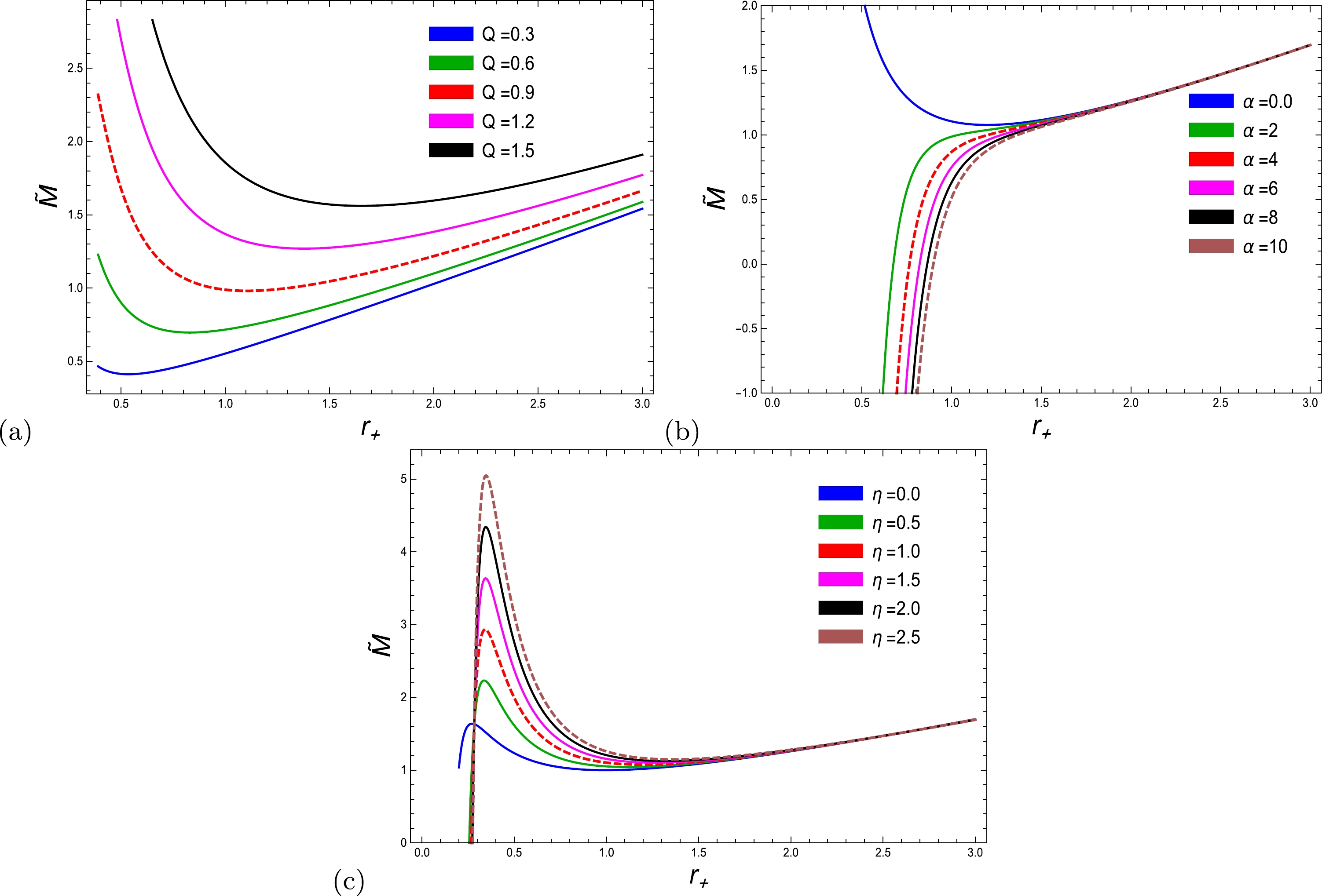
Figure 6. (color online) (Left plots) Internal energy as a function of
$ r_{+} $ with$ l = 20 $ and (a)$ \alpha = 0.02 $ ,$ \eta = 1 $ , (b)$ \alpha = 0.02 $ ,$ Q = 1 $ , and (c)$ Q = 1 $ ,$ \eta = 1 $ .Fig. 6 (a) shows the impact of electric charge on the total corrected mass. We note that the physical corrected mass exhibits a decreasing behavior for the small domain, eventually increasing throughout the considered domain of the horizon radius. As the charge parameter increases, the corresponding physical corrected mass increases with the large BH domain. Fig. 6 (b) shows the impact of the coupling parameter α on the total corrected mass of the EH-AdS BH. It reveals that the phase changes from the negative domain to the positive domain and exhibits stability with increasing radius. Additionally, phase change occurs earlier as α decreases. When
$ \alpha=0 $ , we recover the corrected mass of the RN-AdS BH [12], and in the absence of the coupling parameter, the physical mass remains in the stable region and increases to its maximum with large radii. Fig. 6 (c) states that in the presence of logarithmic first order correction, the associated total corrected mass increases to higher values for short intervals of the horizon radius and starts decreasing for intermediate radii, eventually reaching its peak for large BH radii. Furthermore, a similar behavior can be observed for the corrected mass in the absence of the corrected parameter. It may be noted that the corrected mass under the impact of thermal fluctuations is higher than without correction. In our paper [28], we conducted an analysis of the total corrected mass of the BH under consideration, which was surrounded by a PFDM distribution.It has been observed that as the value of the charge parameter increases, the mass undergoes a transition from the negative to the positive region and remains stable for higher values of the charge parameter. In the initial stages, the energy of the system decreases to the minimum value and subsequently begins to increase for larger radii. The physical mass decreases prior to reaching the critical point, followed by an increase in radius for larger radii. Furthermore, the inclusion of PFDM results in an increase in the internal energy of the system.
In this analysis, the presence of an electric charge has a significant impact on the behavior of the total corrected mass. Specifically, it leads to a decreasing behavior for small domains and an eventual increase throughout the entire considered domain of the horizon radius. With the inclusion of a logarithmic first-order correction, the total corrected mass exhibits an increase toward higher values for small intervals of the horizon radius. This study examines the influence of the coupling parameter on the total corrected mass of EH-AdS BHs. It also investigates the phase transitions from the negative domain to the positive domain and assesses the stability as the radius increases. Furthermore, the phase change occurs at an earlier stage as the coupling parameter decreases. The novel point in BH thermodynamics is the verification of the modified first law of BH thermodynamics. Under thermal fluctuations, the modified first law of thermodynamics can be expressed as
$ \begin{equation} {\rm d}M= \tilde{T}{\rm d}S+\tilde{V}{\rm d}P +\phi {\rm d}Q. \end{equation} $

(33) In the present case,
$ \tilde{T} $ is the corrected Hawking temperature,$ \tilde{V} $ is the corrected volume, and ϕ denotes the electric potential, which are estimated as$ \tilde{T}= \left(\frac{\partial \tilde{M} }{\partial S}\right)_{Q},\,\,\,\,\,\,\,\,\,\,\,\,\ \; \phi=\left(\frac{\partial \tilde{M} }{\partial Q}\right)_{S},\,\,\,\,\,\,\,\,\,\,\,\,\ \; \tilde{V}=\left(\frac{\partial \tilde{M} }{\partial P}\right)_{S, Q} $

The corrected Hawking temperature can be evaluated as
$ \begin{equation} \tilde{T}= \left(\frac{\partial M}{\partial S}\right)_{Q}, \end{equation} $

(34) $ \begin{equation} \tilde{T}= \frac{3 r_+}{4 \pi l^2}+\frac{\alpha Q^4}{16 \pi r_+^7}-\frac{Q^2}{4 \pi r_+^3}+\frac{1}{4 \pi r_+}, \end{equation} $

(35) $ \begin{equation} \tilde{V}= \frac{[35 r_+ \left(\pi r_+^2-6 \eta \right){}^2 \left(6 \alpha \eta l^2 Q^4+\pi \alpha l^2 Q^4 r_+^2-8 \eta l^2 Q^2 r_+^4-4 \pi l^2 Q^2 r_+^6+4 r_+^8 \left(\pi l^2-6 \eta \right)+12 \pi r_+^{10}\right)]}{[6 l^2 \left(180 \alpha \eta ^2 Q^4-6 \pi \alpha \eta \text{r}_+^2 Q^4-140 \pi \eta Q^2 r_+^6+70 \pi ^2 Q^2 r_+^8-7 r_+^4 \left(\pi ^2 \alpha Q^4+40 \eta ^2 Q^2\right)+35 \pi ^2 r_+^{10}\right)]^{-1}}. \end{equation} $ 
(36) The corrected Hawking temperature can be measured using the corrected first law of BH thermodynamics by introducing
$ \tilde{T}=\left(\dfrac{\partial M}{\partial S}_{Q,\alpha}\right) $ . The relative pressure of the charged AdS BH with NLED is given by$ \begin{equation} P= -\frac{{\rm d}F}{{\rm d}\tilde{V}}=-\frac{{\rm d}F/{\rm d}r_+}{{\rm d}\tilde{V}/{\rm d}r_+}, \end{equation} $

(37) With Eqs. (36) and (32), the pressure of the EH BH with NLED takes the form of Eq. (57), as given in the appendix. To investigate the impact of all three parameters regarding the corrected pressure, we depict the graphical behavior of pressure against the BH horizon radius in Fig. 7. Similar work has been conducted in [14, 28, 54, 56, 59, 65] to investigate the corrected pressure for various BHs. Jawad and Shahzad [14] found that the corrected pressure decreased due to the influence of thermal fluctuation. A similar behavior of the corrected pressure was observed in Ref. . The BTZ BH in [54] showed that there was a significant impact of thermal fluctuation for small horizon radii; however, for BHs with large horizon radii, the pressure was not significantly affected by thermal fluctuation. Remarkably, it was observed that in the absence of logarithmic correction, the pressure in BH thermodynamics behaved like an ideal gas, whereas in the presence of thermal fluctuation, the pressure acted as a van der Waal gas [56]. Fig. 7 (a) describes the consequences of the charge parameter to express the corrected pressure. We find that for the large altered values of the charge parameter from
$ Q=0.90 $ to$ Q=1.50 $ , phase change occurs from a negative range to a positive range on its peak for short radii, whereas at$ Q=0.30 $ and$ Q=0.60 $ , the pressure remains positive and moves from the highest level toward equilibrium. Hence, the overall trend is to move from a stable region to its equilibrium state. From Fig. 7 (b), it is clear that the overall trend of the corrected pressure about the instability is to diverge with the distinct values of the coupling parameter as well as in the absence of the coupling parameter. Fig. 7 (c) describes the pressure with and without the impact of the corrected parameter η. As a whole, phase transition occurs from an unstable region to a stable region when$ \eta=0 $ with different values of the coupling parameter. Moreover, there are some divergences for particular values of η, such as$ \eta=2 $ and$ \eta=2.5 $ . Therefore, comprehensively, for small domains, pressure increases to its maximum and decreases toward equilibrium for large radii.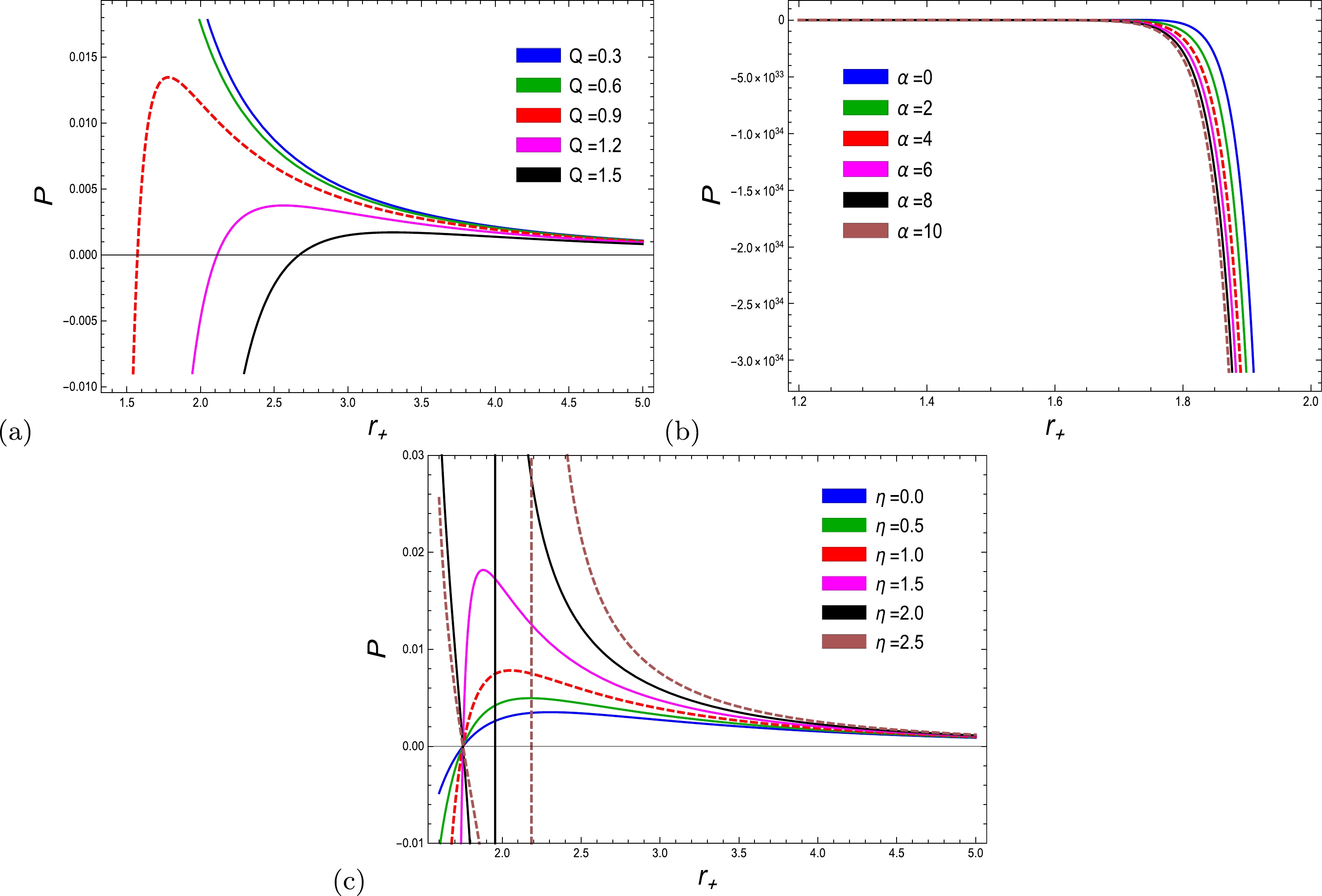
Figure 7. (color online) Pressure as a function of
$ r_{+} $ with$ l = 20 $ and (a)$ \alpha = 0.02 $ ,$ \eta = 1 $ , (b)$ \alpha = 0.02 $ ,$ \eta = 1 $ , and (c)$ Q = 1 $ ,$ \eta = 1 $ .As presented in our recently published paper [28], we observed that the corrected pressure exhibited an initial decrease at smaller values of the charge parameter. This modified pressure then reached the equilibrium state for fixed values of the PFDM and correction parameters. For higher values of the charge parameter, a second-order phase transition was observed, characterized by a transition from a stable state to an unstable state, followed by a return to stability.
Based on our present evaluation, for a significant range of the charge parameter, a phase change occurs from a negative range to a positive range at the peak for shorter radii. Conversely, the pressure remains positive and gradually moves from the highest level to equilibrium. Therefore, there is a prevailing tendency to transition from a state of stability to a state of equilibrium. In summary, in the case of a smaller horizon radius, the pressure reaches its maximum value and gradually decreases toward equilibrium as the radius increases. It is evident that the general trend of the corrected pressure regarding instability is to diverge with varying values of the coupling parameter, and such behavior would occur in the absence of the coupling parameter.
The enthalpy of a system or its total heat content is a fundamental thermodynamic quantity. The enthalpy can be redefined as
$ \begin{equation} H= \tilde{M}+PV. \end{equation} $

(38) The simplified form of the above equation is given in Eq. (58) in the appendix.
In terms of visual behavior, enthalpy is associated with the horizon radius, as illustrated in Fig. 8. The enthalpy justifies the stability of the system for all parameters and for all located domains. Thermal fluctuation only affects small radii, whereas there is no effect on larger radii. There have been numerous [14, 28, 54, 56, 61−63] finding on the enthalpy of BHs. In literature [54], it has been established that with an increase in the value of the correction parameter, the resulting enthalpy decreases and vice versa. The enthalpy is an increasing function of the horizon radius with and without the existence of the correction parameter. Evidently, the effect of thermal fluctuation on a small domain is remarkably significant, as discussed in Ref. [56]. A similar behavior of enthalpy has been observed in [62, 63]. In Fig. 8 (a), the enthalpy is the increasing function regarding the charge parameter, and as the various values of the charge parameter increase, the respective enthalpy also increases. For particular values of the coupling parameter, phase space exists from the domain of instability to stability and rises to maximality with a large domain in Fig. 8 (b). Moreover, when
$ \alpha=0 $ , the graph describes the enthalpy of the RN-AdS BH [12], and there is a critical point at$ r_{+}=1.25 $ , for which the enthalpy becomes negative before the critical point and increases after the critical horizon radius. There are some discontinuities at small radii at large values of the correction parameter η at$ \eta=1.50 $ to$ \eta=2.50 $ in Fig. 8 (c). Subsequently, the above values of enthalpy decrease to their minima and then gradually increase to their maxima for large radii. With the correction parameter$ \eta=0 $ ,$ \eta=0.50 $ , and$ \eta=1 $ , the system remains stable throughout the considered domain.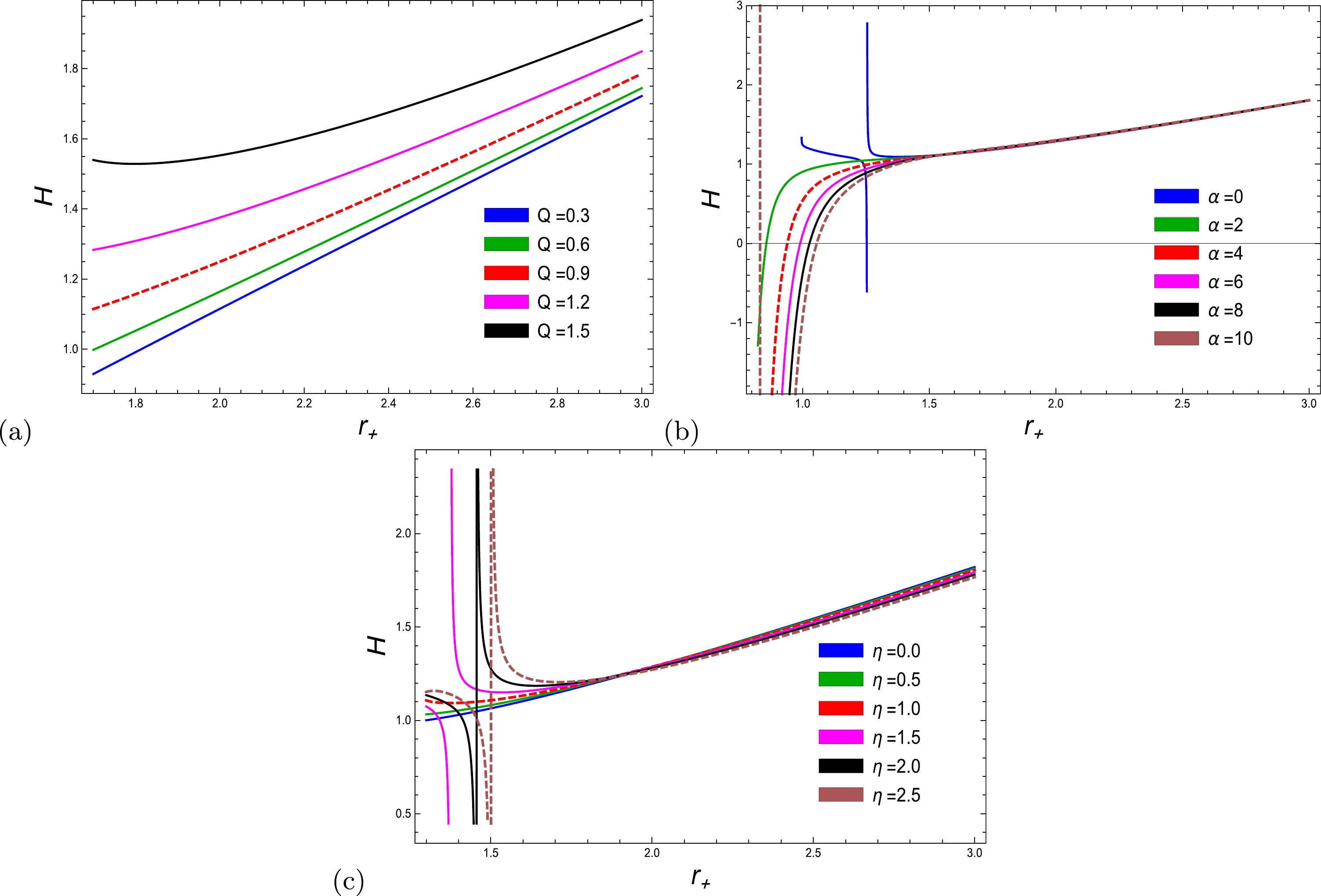
Figure 8. (color online) Enthalpy as a function of
$ r_+ $ with$ l=20 $ and (a)$ \alpha=0.02 $ ,$ \eta=1 $ , (b)$ \alpha=0.02 $ ,$ Q=1 $ , and (c)$ Q=1 $ ,$ \eta=1 $ .The findings of a previously published paper [28] indicated that the system exhibited a consistent positive increase for large BH radii. The enthalpy of the system exhibited a decrease to a minimum for small horizon radii prior to reaching the critical horizon radius. Subsequently, after surpassing the critical point, the enthalpy gradually increased toward its maximum value. The enthalpy demonstrated stability in the presence of the PFDM parameter.
In the present study, the enthalpy is a function that increases with respect to the charge parameter. As the charge parameter increases, the corresponding enthalpy values also increases. The system maintains stability within the specified domain for the correction parameters
$ \eta = 0 $ ,$ \eta = 0.50 $ , and$ \eta = 1 $ . For specific values of the coupling parameter, a phase space exists and transition occurs from a domain of instability to stability, eventually reaching maximality with a large domain. Notably, there is a critical point located at$ r_{+} = 1.25 $ , where the enthalpy transition would occur from negative values to increasing values of the horizon radius beyond the critical horizon radius. To illustrate the global stability, the Gibbs free energy is an important factor. The Gibbs free energy$ G= H-TS $ takes the form of Eq. (59), which is given in the appendix.For the global stability, the graphical behavior of Gibbs free energy with respect to all three parameters is displayed in Fig. 9. More information about the Gibbs free energy of various BHs can be found in Refs. [14, 28, 54, 64, 65]. The first two plots of Gibbs free energy explore the analogy with enthalpy, as mentioned above. Fig. 9 (c) identifies the monotonically increasing response for small-to-large radii and for the corrected and uncorrected Gibbs free energy. It can be noted that the amount of free energy in the absence of the correction parameter is larger than the Gibbs free energy with the correction parameter for small to large radii. Thus, a BH with a large horizon radius has a positive Gibbs free energy for all parameters.
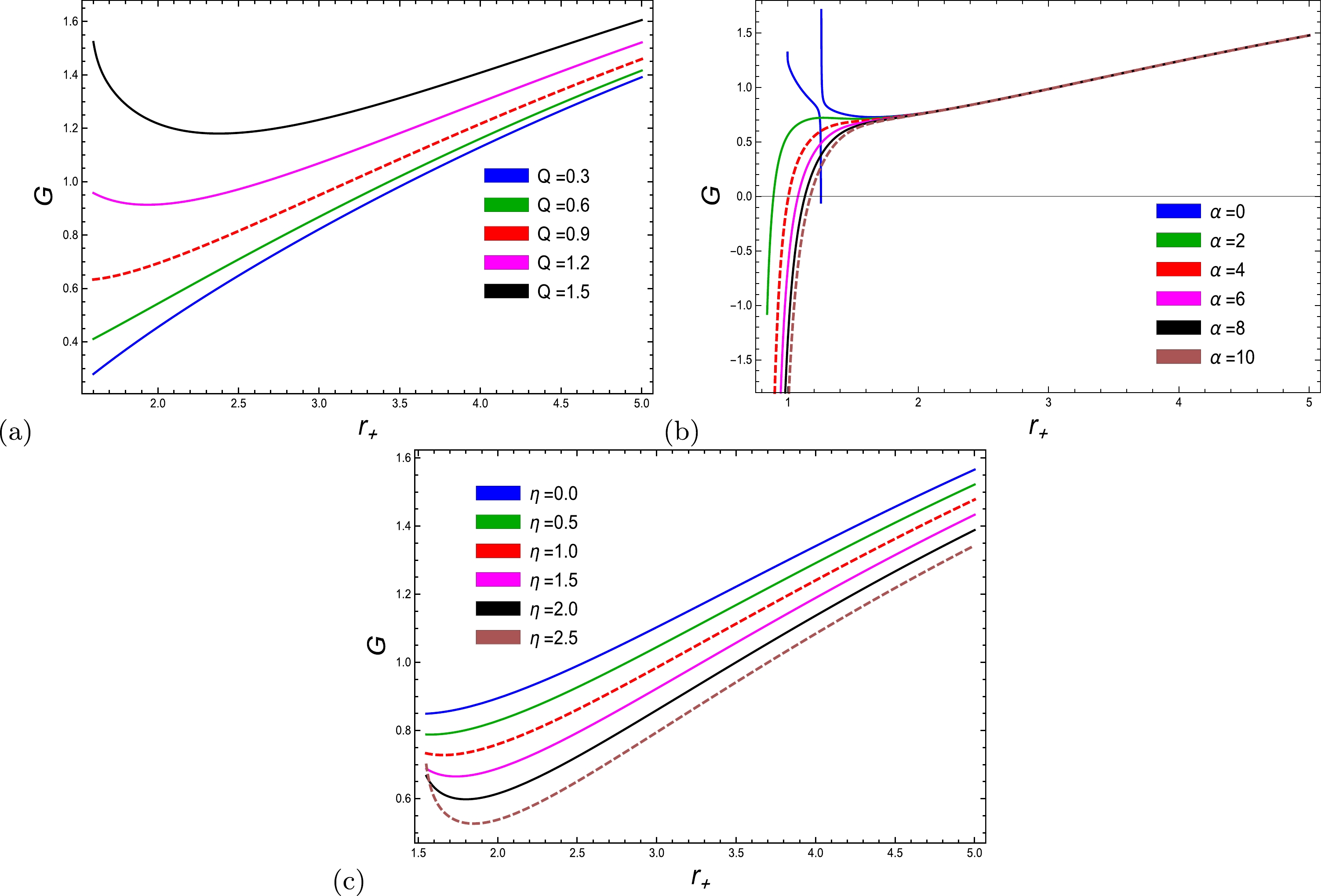
Figure 9. (color online) Trace of the Hessian matrix as a function of
$ r_+ $ with$ l=20 $ and (a)$ \alpha=0.02 $ ,$ \eta=1 $ , (b)$ \alpha=0.02 $ ,$ Q=1 $ , and (c)$ Q=1 $ ,$ \eta=1 $ .In the graph in Ref. [28], the Gibbs free energy increases to its maximum value across the entire range under consideration. There is no pattern between the corrected and uncorrected free energy; however, it is clear that the uncorrected Gibbs free energy is larger than the corrected free energy. To facilitate a discussion on the Gibbs free energy with respect to different values of the PFDM parameter, it is evident that the free energy becomes increasingly stable and significant with higher values of the charge parameter. In the present case, Gibbs-free energy is a crucial factor for demonstrating the global stability. The charge parameter exhibits a monotonically increasing response for small-to-large radii, both with and without the correction of Gibbs free energy. It is worth noting that the free energy in the absence of the correction parameter is greater than the Gibbs free energy with the correction parameter for radii ranging from small to large. Therefore, a BH with a significant horizon radius exhibits a favorable Gibbs free energy value for all the BH parameters. To study the local stability of the charged EEH BH, specific heat,
$ C {s}=T\dfrac{{\rm d}S}{{\rm d}T} $ , is used. We evaluate the thermal stability using the corrected specific heat of the EEH BH with NLED, which is given by$ C_s=-\frac{2 \left(6 \alpha \eta l^2 Q^4+\pi \alpha l^2 Q^4 r_+^2-8 \eta l^2 Q^2 r_+^4-4 \pi l^2 Q^2 r_+^6+4 r_+^8 \left(\pi l^2-6 \eta \right)+12 \pi r_+^{10}\right)}{7 \alpha l^2 Q^4-12 l^2 Q^2 r_+^4+4 l^2 r_+^6-12 r_+^8}. $

The physical interpretation of specific heat vs. the horizon radius of the EEH-AdS BH is shown in Fig. 10. Many studies, including [14, 28, 56, 64, 65], have looked into the role of heat capacity in determining regional stability. To investigate the local stability [14] of the BH thermodynamic system, we must describe the sign of specific heat. The stability of a system is indicated by a positive value of specific heat capacity (if
$ C>0 $ ), whereas instability is indicated by a negative value (if$ C<0 $ ). In , an unstable (stable) phase occurred for small BHs (large BHs) owing to the remarkable influence of logarithmic correction. Furthermore, owing to the correction term, stability was found to occur for small BHs. Pourhassan and Upadhyay [64] concluded that in the absence (presence) of logarithmic correction, the small BHs remained unstable (stable). They also observed a phase transition from stability to instability due to the correction parameter. Fig. 10 (a) describes the heat capacity in a stable region for small BH horizon radii, and for large radii, the heat capacity moves into a negative region and become unstable. For the coupling parameter, it is suggested that heat capacity moves down to the negative range for increasing values, whereas in the absence of the coupling parameter α, the phase change describes the stability for the heat capacity, as depicted in Fig. 10 (b). From the corrected parameter perspective, the corresponding heat capacity in Fig. 10 (c) suggests that corrected specific heat is still stable throughout the system for small radii before the critical horizon radius at$ r_{+}=r_{c} $ , and after this critical point, the specific heat preserves instability for large radii. In [28], we examined the concept of specific heat as a means of analyzing the local stability of the BH. The phase transitions occurred exclusively for small values of the charge parameter with a small BH horizon radius. To assess the influence of the logarithmic correction resulting from thermal fluctuation, our study focused on characterizing the phase transition occurring prior to the critical radius$ r_{c} = 1 $ . It is evident that the heat capacity initially diverged from the negative region to the positive one to reach its maximum value.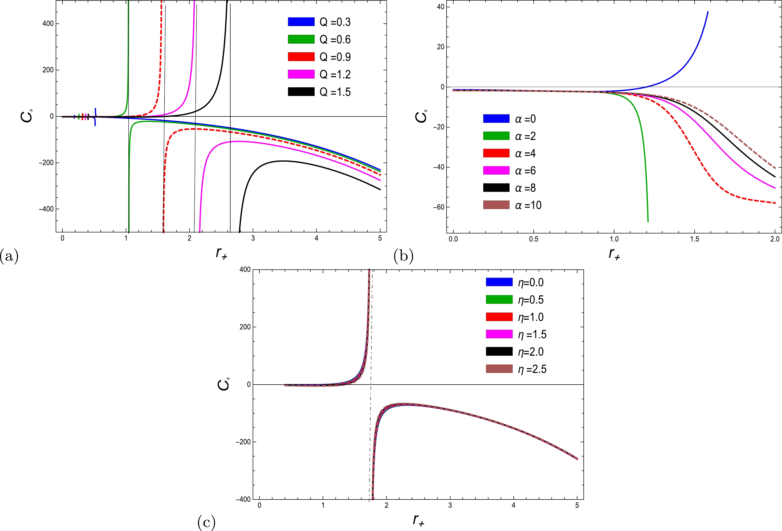
Figure 10. (color online) Gibbs free energy as a function of
$ r_+ $ with$ l=20 $ and (a)$ \alpha=0.02 $ ,$ \eta=1 $ , (b)$ \alpha=0.02 $ ,$ Q=1 $ , and (c)$ Q=1 $ ,$ \eta=1 $ .In the present analysis, the charge parameter is used to characterize the heat capacity within a stable region for small BH horizon radii. However, for larger radii, the heat capacity changes its phase to a negative region, rendering it unstable. From the perspective of the corrected parameter, the heat capacity indicates that the corrected specific heat remains constant within the system for small radii. However, once the critical horizon radius is reached at
$ r_{+} = r_{c} $ , the specific heat becomes unstable for larger radii. In relation to the coupling parameter, the heat capacity exhibits a negative trend as the parameter increases. Conversely, in the absence of the coupling parameter, the stability of the heat capacity is described by phase change.For charged BHs, the sign of specific heat is insufficient; therefore, the Hessian matrix of the Helmholtz free energy is needed to test the stability. The Hessian matrix H is also used to measure the stability of the system, which involves the second-order derivatives of the Helmholtz free energy. The Hessian matrix [10] can be written as
$ \begin{equation} H=\left( \begin{array}{cc} H_{ii} & H_{ij} \\ H_{ji} & H_{jj} \\ \end{array} \right) =\left( \begin{array}{cc} H_{11} & H_{12} \\ H_{21} & H_{22} \\ \end{array} \right)\,\,\,\,\,\,\, i,j=1,2 \end{equation} $

(39) where
$ H_{11}=\dfrac{\partial^{2}F}{\partial T^{2}} $ ,$ H_{12}=\dfrac{\partial^{2}F}{\partial T \partial\phi} $ ,$ H_{21}=\dfrac{\partial^{2}F}{\partial\phi\partial T },\; H_{22}=\dfrac{\partial^{2}F}{\partial \phi^{2}} $ . It is constructive to acknowledge that the stability of the system can be determined by the trace of the Hessian matrix$ T_{r}(H)=H_{11}+H_{22} \geq 0 $ . Because$ H_{ii}H_{jj} = H_{ij}H_{ji} $ , one of the Hessian matrix eigenvalues must be zero. We use the trace of the Hessian matrix to conclude the stability of the geometry. The elements of the Hessian matrix are$ \begin{aligned}[b] \\ H_{11}= \frac{16 \pi l^2 r^8 }{l^2 (-7 \alpha Q^4+12 Q^2 r^4-4 r^6)+12 r^8}\Bigg(\frac{4 \eta (l^2 (4 Q^2 r^4-3 \alpha Q^4)+12 r^8)}{l^2(\alpha Q^4 r-4 Q^2 r^5+4 r^7)+12 r^9}-2 \pi r)\Bigg),\end{aligned} $ 
$ \begin{aligned}[b] H_{22}=&\Big(8 \pi r^6 (l^2(-11 \alpha Q^4+9 \alpha Q^2 r^2-2 r^6)+12 r^4(r^4-3 \alpha Q^2))-6 \eta (l^2 Q^2 (7 \alpha ^2 Q^4-2 \alpha r^4(Q^2+4 r^2)\\&+8 r^8)+36 \alpha Q^2 r^8-8 r^{12})(\log (256 \pi l^4 r^{12})-2 \log(l^2(\alpha Q^4-4 Q^2 r^4+4 r^6)+12 r^8)) \\ &-\Big(l^2 (\alpha Q^4-4 Q^2 r^4+4 r^6)+12 r^8\Big)^{-1}(4 \eta (2 r^4-3 \alpha Q^2)(l^2(-7 \alpha Q^4+12 Q^2 r^4-4 r^6)+12 r^8)\\& (l^2 (4 Q^2 r^4-3 \alpha Q^4)+12 r^8))\Big)\Big(r^3\Big(4 \pi l^2 (2 r^4-3 \alpha Q^2)^2(3 \alpha Q^2-2 r^4)\Big)^{-1}\Big). \end{aligned} $

(40) The trace of the Hessian matrix is given by Eq. (60) in the appendix. The trace of the Hessian matrix is a technique for checking the stability, as represented in Fig. 11. Many researchers [10, 28, 61, 63, 65] have used this technique to determine stability. With distinct values of electric charge parameters, the trace of the Hessian matrix is only favorable for the stability of large horizon-radius BHs and exhibits divergences for small horizon-radius BHs. This reveals that thermal fluctuation affects small BHs, as shown in Fig. 11 (a). From the perspective of the coupling parameter in Fig. 11 (b), the trace of the Hessian matrix exhibits discontinuities for small radii, and for the large domain of the considered BH, a phase space shift from an unstable region toward a stable one. Furthermore, when
$ \alpha=0 $ , the blue line reveals stability, which decreases for short radii before increasing again. The trace of the Hessian matrix becomes divergent at the critical radius$ r_{c}=1.80 $ . Fig. 11 (c) describes the effect of thermal fluctuation only for small-radius BHs, and after the critical radius, there is no effect of thermal fluctuation for various values of the EH parameter.
Figure 11. (color online) Corrected specific heat as a function of r with
$ l=20 $ and (a)$ \alpha=0.02 $ ,$ \eta=1 $ , (b)$ \alpha=0.02 $ ,$ Q=1 $ , and (c)$ Q=1 $ ,$ \eta=1 $ . -
In this section, we discuss the phase transition of the Hawking temperature and heat capacity for the EH-AdS BH with NLED against entropy. Using Eqs. (17) and (27), the Hawking temperature takes the form
$ \begin{equation} T= \Bigg(\frac{l^2 \left(\alpha Q^4-4 Q^2 r_+^4+4 r_+^6\right)+12 r_+^8}{16 l^2 r_+^5 S_0} \Bigg). \end{equation} $

(41) Using Eqs. (28) and (17), the heat capacity of the EH-AdS BH with NLED is given by
$ \begin{equation} C= \Bigg(\frac{2 S_0 \left(l^2 \left(\alpha Q^4-4 Q^2 r_+^4+4 r_+^6\right)+12 r_+^8\right)}{l^2 \left(-7 \alpha Q^4+12 Q^2 r_+^4-4 r_+^6\right)+12 r_+^8}\Bigg). \end{equation} $

(42) Figure 12 (left plots) comprises the physical aspect of the Hawking temperature of the EH-AdS BH along with NLED against entropy, which identifies the phase transition with distinct values of charge, radial distance, and the coupling parameter of the EH BH. Work of a similar nature was used to obtain the phase transition that corresponds to the usual entropy in Refs. [28, 61, 63]. When Q and
$ r_{+} $ are increased, the Hawking temperature goes from being positive to negative. As the NLED parameter is increased, the Hawking temperature experiences a phase change from negative to positive. When the values of Q,$ r_{+} $ , and the NLED parameters are increased, the phase of the heat capacity of the BH shifts from negative to positive. It has also been noticed that the considered system exhibits unstable behavior for small values of the considered parameters, whereas for large values, it demonstrates stable behavior. With different parametric values, phase changes occur from positive (negative) to negative (positive) in Hawking temperature. The temperature changes its state from positive to negative with increasing values of Q, as shown in Fig. 12 (a), whereas in Fig. 12 (b) and (c), the phase transition of Hawking temperature is from negative to positive with decreasing values of$ r_{+} $ and the EH parameter. The right plots of Fig. 12 indicate the behavior of specific heat against entropy, which establishes a phase transition with the presence of Q,$ r_{+} $ , and α. With higher values of the charge parameter in Fig. 12 (d), heat capacity changes from unstable to stable, and with higher values of$ r_{+} $ and the nonlinear parameter in Fig. 12 (e) and Fig. 12(f), heat capacity changes from a negative phase to a positive phase.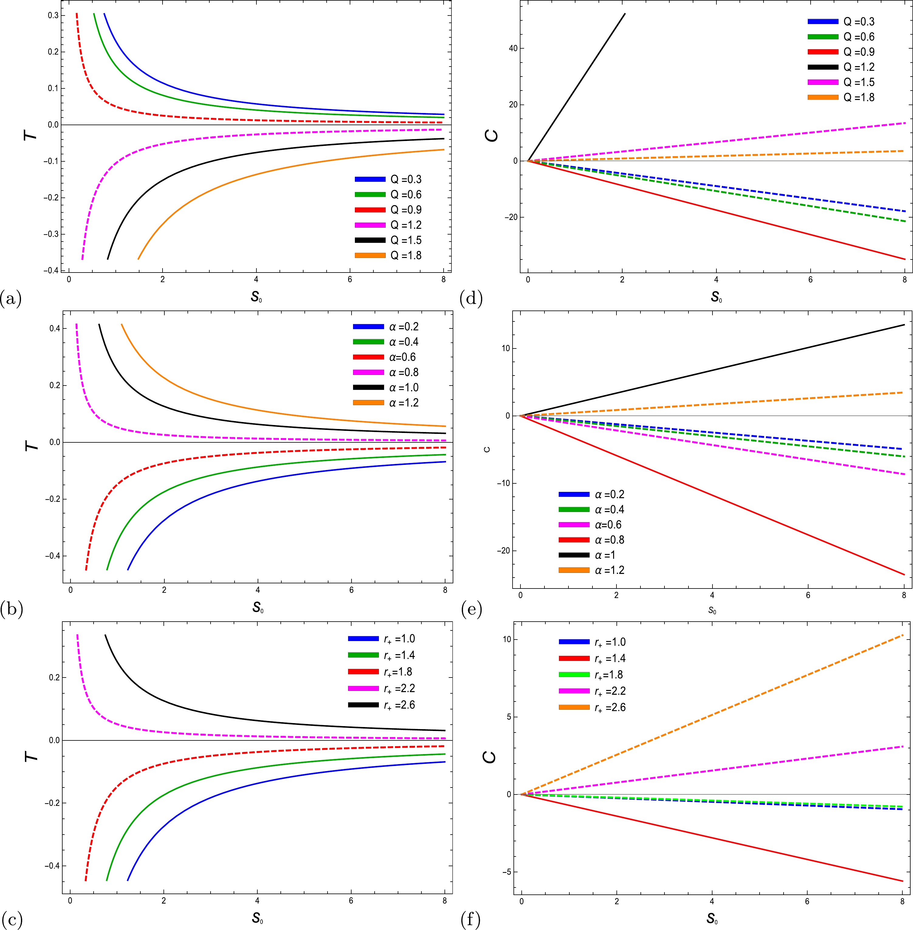
Figure 12. (color online) (Left plots) Temperature as a function of
$ S_0 $ with$ l=20 $ and (a)$ r=1 $ ,$ \alpha=0.02 $ , (b)$ \alpha=0.02 $ ,$ Q=2 $ , and (c)$ Q=2 $ ,$ r=1 $ . (Right plots) Heat capacity as a function of$ S_0 $ with$ l=20 $ and (d)$ r=2 $ ,$ \alpha=1 $ , (e)$ \alpha=1 $ ,$ Q=2 $ , and (f)$ Q=3 $ ,$ r=1.5 $ . -
The study of the relationship between the phase transition and QNMs is an important first step toward understanding BH thermodynamics. In this section, we discuss null geodesics and the sizes of photon spheres in relation to the EH BH with NLED. We investigate how free photons move in the background of the BH. The geodesics surrounding BHs consist of various closed and open orbits, which are determined by their relative positions with respect to the BHs. Orbits can exhibit stable and unstable behavior. The stability of geodesics can be assessed by employing the Lyapunov exponent [ 66] as a measure. The Lyapunov exponent plays a significant role in the field of GR owing to its wide range of applications and is a highly influential mathematical entity that is valuable for analyzing systems with chaotic dynamics, commonly observed in nonlinear systems. Additionally, this tool can be used to examine the stability of particle trajectories. The Lyapunov exponent is mathematically characterized as the mean rate at which two adjacent geodesics or geodesic congruences can either converge or diverge within the phase space [67]. In the event that the Lyapunov exponent is positive, it can be concluded that the system exhibits chaotic behavior. This implies that even minor disturbances experience exponential growth, leading to unpredictable system dynamics over time. In the event that the Lyapunov exponent is negative, the system is considered stable. This implies that minor disturbances tend to converge toward a fixed point or a periodic orbit. The vanishing of the Lyapunov exponent signifies that the rate of divergence or convergence of nearby trajectories tends toward zero, suggesting that the system is marginally stable. A geodesic stability analysis in terms of the Lyapunov exponent begins with the equations of motion. We focus on the analytical formulation of the Lyapunov exponent and QNMs in terms of the expressions of the radial equation of circular geodesics about a BH space-time. In this regard, an equatorial circular geodesic about a BH may play a crucial role in the general theory of relativity for the classification of orbits. In literature [68−70], the Lyapunov exponent has been studied for the instability of circular null geodesics in terms of the expressions for the QNMs of spherically symmetric space-time. The primary emphasis is placed on the null circular geodesics, which hold significant importance in relation to the Lyapunov exponent. The null circular geodesics are characterized by the minimum orbital period, as determined by asymptotic observers [71]. The WKB method provides a precise estimation of the frequency of QNMs in the eikonal limit. The WKB method was initially introduced by Schutz and Will [72] to analyze the scattering problem of BHs. The eikonal approximation is employed for the investigation of the QNMs associated with a BH. These modes are important for understanding the behavior of BHs and testing various theories of gravity. In the context of the eikonal approximation, the BH is regarded as a geometric entity characterized by a well-defined shape and distribution of mass. The QNMs can be determined by solving the wave equation for minor disturbances in the BH geometry. The eikonal approximation is based on the assumption that the wavelength of the perturbation is significantly smaller than the radius of the BH horizon. The utilization of the eikonal approximation yields an approximate formulation for the QN frequencies of the BH, contingent upon the characteristics of the BH. The eikonal approximation continues to be a valuable tool for investigating the QNMs of BHs and gaining insights into the dynamics of gravity in the vicinity of strong BH gravitational fields. The link between QNMs and unstable circular null geodesics is a broad one because it holds true in the eikonal limit for any space-time that is static, spherically symmetric, and asymptotically flat. In our study, we demonstrate the agreement between the angular velocity at the unstable null geodesic and the Lyapunov exponent, which determines the instability timescale of the orbit, with the analytic WKB approximations for QNMs [73, 74]. Therefore, in general, QNMs can only be used to make sense of unstable circular null geodesics in space-times that are spherically symmetric and asymptotically flat. When evaluating the angular velocity of a photon and the Lyapunov exponent, we use the radius of the photon sphere as our point of reference. It is possible to interpret the motion as staying within the equatorial plane (
$\theta= {\pi}/{2}$ ). For a photon, the Lagrangian becomes$ \begin{equation} \mathcal{L}=N(r)\dot{t}^2- N(r)^{-1}\dot{r}^2-r^2 \dot{\phi}^2, \end{equation} $

(43) where ϕ represents the angular coordinate. The corresponding components of generalized momenta
$\bigg (\widetilde{P}_{\nu}=g_{\nu\mu}\dot{x}^{\mu}- \dfrac{\partial\mathcal{L}}{\partial\dot{x}^{\nu}}\bigg)$ are defined as$ \begin{equation} \widetilde{P}_t=E= N(r)\dot{t}= constant, \end{equation} $

(44) $ \begin{equation} \widetilde{P}_r=\frac{\dot{r}}{N(r)}, \end{equation} $

(45) $ \begin{equation} \widetilde{P}_{\phi }=-r^2\dot{\phi}=-l= constant, \end{equation} $

(46) where the conserved constants E and l describe the energy and angular momentum of the photon, respectively. From Eq. (44), the Eq. (46) can be estimated as
$ \dot{t}=\dfrac{E}{N(r)} $ ,$ \dot{\phi}=\dfrac{l}{r^2}. $ The related Hamiltonian equation for the null geodesicsbecomes$ \begin{equation} \mathcal{H}= N(r)\dot{t}^2-N(r)^{-1}\dot{r}^2 \dot{\phi}^2= E\dot{t}-l\dot{\phi}-\frac{\dot{r}^2}{N(r)}, \end{equation} $

(47) which leads to
$ \begin{equation} V_{e}=-{\dot{r}^2}, \end{equation} $

(48) with
$ \begin{equation} V_{e}= -E^{2}+\frac{l^{2}}{r^2}N(r). \end{equation} $

(49) For spherically symmetric static space-time, there are also some unstable circular orbits of photon spheres that can be found by meeting the following three conditions:
$ \begin{equation} V_{e}=0,\,\,\,\,\,\,\,\,\,\,\,\ \frac{\partial V_{e}}{\partial r}=0\,\,\,\,\,\,\,\,\,\,\ \frac{\partial^{2}V_{e}}{\partial r^{2}}<0. \end{equation} $

(50) Solving Eqs. (49) and (50), we obtain the required result as follows:
$ \begin{equation} \frac{\partial V_{e}}{\partial r}=-r_{ps}N'(r_{ps})+2N(r_{ps})=0. \end{equation} $

(51) Using the respective metric function from Eq. (16), Eq. (50) takes the form
$ \begin{equation} 5r_{ps}^{6}+10Q^{2}r_{ps}^{4}-15M2r_{ps}^{5}-\alpha Q^{4}=0. \end{equation} $

(52) According to the eikonal limit
$ l>>1 $ , the QNMs can be revealed with the help of the photon sphere as under$ \begin{equation} \omega_{Q}=\Omega l-\iota\left| \lambda \right|\left(\frac{2n+1}{2}\right), \end{equation} $

(53) Eventually, the QNMs are coupled with the angular velocity Ω and Lyapunov exponent Γ as
$ \begin{equation} \Omega=\frac{\sqrt{N_{ps}}}{r_{ps}}, \,\,\,\,\,\,\,\,\,\, \Gamma= \sqrt{-\frac{V''_{\text{e}}}{2 \dot{t}^2}}, \end{equation} $

(54) which produces
$ \begin{aligned}\\ \Omega=\frac{1}{2 \sqrt{5} l r_{ps}^4}\Big(\sqrt{-40 l^2 m r_{ps}^5-\alpha l^2 Q^4+20 l^2 Q^2 r_{ps}^4+20 l^2 r_{ps}^6+20 r_{ps}^8} \Big), \end{aligned} $ 
(55) and
$ \begin{aligned}\\ \Gamma=\frac{1}{2 \sqrt{5} l r_{ps}^7}\Big(\sqrt{\left(\alpha Q^4-2 Q^2 r_{ps}^4+r_{ps}^6\right) \left(l^2 \left(20 r_{ps}^5 (r_{ps}-2 m)-\alpha Q^4+20 Q^2 r_{ps}^4\right)+20 r_{ps}^8\right)}\Big). \end{aligned} $

(56) Figure 13 shows the physical behavior of angular velocity and the Lyapunov exponent in terms of electric charge. The graphical behavior of angular velocity versus Q demonstrates that the coupling parameter significantly affects the angular velocity of the photon. Moreover, it has been noticed that the photon angular velocity is not defined until the value of charge is
$ Q = 1 $ . As the domain becomes larger, the angular velocity and coupling parameter are the opposites of each other in Fig. 13 (a). On the other hand, as shown in Fig. 13 (b), the relationship between the rate of increase in angular velocity and the radius of the photon sphere is inverse. As shown in Fig. 13 (c), the Lyapunov exponent exhibits a trend of increasing behavior for decreasing values of coupling parameters with an increasing domain. The behavior of the Lyapunov exponent is shown to be increasing in Fig. 13 (d), which corresponds to an increasing photon sphere radius.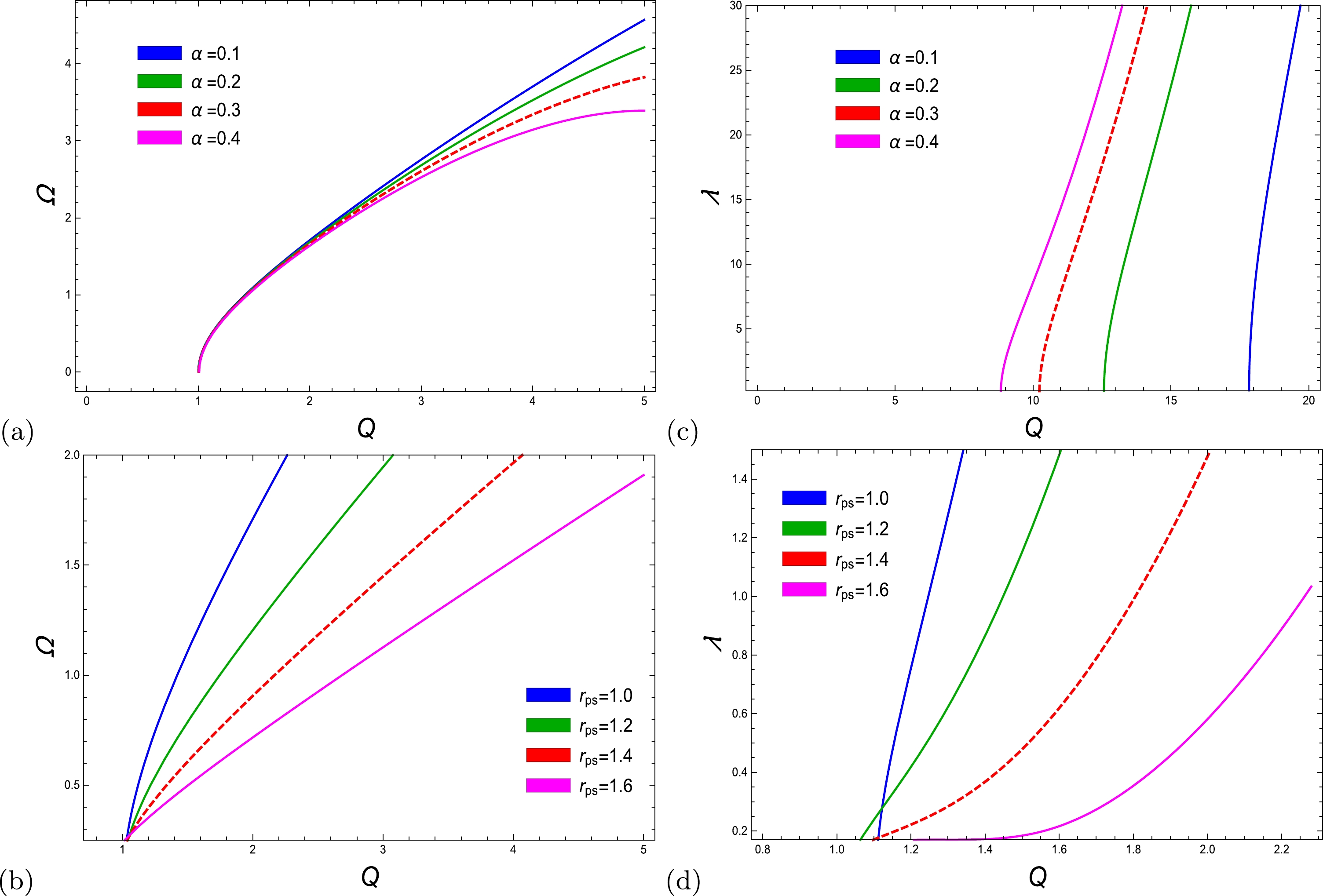
Figure 13. (color online) (Left plots) Angular velocity as a function of Q with
$ l=20 $ ,$ M=1 $ and (a)$ r_{ps}=1 $ , and (b)$ \alpha=0.10 $ . (Right plots) Lyapunov exponent as a function of Q with$ l=20 $ ,$ M=1 $ and (c)$ r_{ps}=2 $ , and (d)$ \alpha=3 $ . -
This paper investigates the thermodynamical variables, such as Hawking temperature, entropy, and specific heat, of EH-AdS BHs under the effects of NLED. Graphically, it is observed that the validity is complete and all these quantities obey the first law of thermodynamics. To examine the impact of thermal fluctuation with simple logarithmic correction for EH-AdS BHs with NLED, we measure thermodynamical potentials, such as corrected entropy, corrected temperature, Helmholtz free energy, total corrected mass, Gibbs free energy, thermodynamical pressure, enthalpy, heat capacity, and the trace of the Hessian matrix. It is worth noting that all these corrected quantities agree with the first law of thermodynamics under the influence of thermal fluctuation with a simple logarithmic correction. The stability and physical behavior of all physical quantities, such as heat capacity and the Hessian matrix, are also depicted. Moreover, we evaluate the phase transition of temperature and heat capacity associated with entropy. The physical behavior is illustrated for these quantities with the correction/NLED parameter to observe the impact of the correction parameter. First, using surface gravity, we obtain the Hawking temperature and specific heat. Graphically, we find that BHs with small radii are stable, whereas BHs with large radii are unstable for specific heat. Second, the corrected entropy reveals a stable trend and reaches its maximum values for large radii BHs. The increasing behavior of the corrected entropy implies an increase in its area in BH geometry via the area-entropy relation. This phenomenon gives us information about the extraction of further work. The corrected Hawking temperature coincides with the Hawking temperature without correction. The Helmholtz free energy monotonically increases with increasing trends in charge and correction parameters. The physical behavior of Helmholtz free energy under the effect of the EH parameter describes the system reaching its peak for small and large BHs. The graphical trend of the total corrected mass presents a positive state, which implies that the BH absorbs heat energy from its vicinity. The EH parameter demonstrates that stability increases more rapidly as the values of the parameter decrease in the first phase to show its stability and indicate that more energy can be absorbed from the surrounding area. It is noted that the corrected pressure changes its phase from instability toward equilibrium with larger values of parameters, whereas the impact of the EH parameter shows a decreasing trend throughout the system and remains unstable. The graphical depiction of enthalpy illustrates a stable state for all the parametric values of the charge and correction parameters. However, the NLED parameter reveals the phase change from a negative to a positive state. Third, the specific heat and the trace of the Hessian matrix are investigated. As well as QNMs and null geodesics, we calculate the real part, which is considered as angular velocity, and the imaginary part, which is the Lyapunov exponent. It is important to note that all results reduce to RN-AdS BHs when
$ \alpha=0 $ [12].By comparing the results of our current paper with the work presented in [28], we reach the following conclusions:
$ 1 $ - As the coupling parameter increases, the entropy of large-radius BHs becomes more stable in comparison to small-radius BHs. The current study demonstrates the physical significance and novelty of the relationship between the coupling parameter and the corrected entropy in the entire domain. It is observed that higher values of the coupling parameter correspond to higher corrected entropy.$ 2 $ - This investigation is significant owing to its physical implications and novelty. The Helmholtz-free energy remains stable in entire domain and reaches its maximum value when the correction parameter is absent. The EH coupling parameter provides insight into the phase transition occurring within the system, specifically the transition from an unstable region to a stable one.$ 3 $ - The present analysis emphasizes the significance and novelty of showcasing the preservation of a positive and stable total corrected mass for the designated values of the charge parameter within the provided domain. The correction parameter manifests variations in its phase and exhibits both ascending and steady characteristics. The EH coupling parameter serves as an indicator of the corrected mass and describes the transition from a negative to a positive phase within a specific region. Moreover, in the realm of astrophysics, when the coupling parameters exhibit diminutive values, the phase transition transpires with augmented celerity.$ 4 $ - This manuscript holds great significance and novelty because it elucidates the profound influence of altering the charge parameter values on the stability of the corrected pressure. The correction parameter exhibits enhanced stability for larger radii once more. The examination of the coupling parameter reveals that the system displays instability within the designated domains.$ 5 $ - This investigation holds great significance and novelty because it showcases the profound influence of modifying charge parameter values on the stability of the corrected pressure. Once again, the correction parameter exhibits enhanced stability as the radius increases. The examination of the coupling parameter suggests that the system demonstrates instability within the designated domains.$ 6 $ - The charge parameter carries immense astrophysical significance and novelty because it leads to the manifestation of a positive and escalating trend in the Gibbs free energy of the system. It is crucial to acknowledge the occurrence of the phase transition from the negative region to the positive region.$ 7 $ - The remarkable feature of this study is that the existence of a coupling parameter results in the divergence of the heat capacity, signifying an inherent state of instability. In the absence of the coupling parameter, the heat capacity asymptotically approaches a region of thermodynamical stability. -
$ \begin{aligned}[b]\\ P=&\Big(-((3(-7 \alpha l^2 Q^4+12 l^2 Q^2 r_+^4-4 l^2 r_+^6+12 r_+^8)(\eta (\log (256 \pi l^4 r_+^{12})-2 \log (\alpha l^2 Q^4-4 l^2 Q^2 r_+^4+4 l^2 r_+^6+12 r_+^8))+\pi r_+^2)\\&(180 \alpha \eta ^2 Q^4-6 \pi \alpha \eta Q^4 r_+^2-140 \pi \eta Q^2 r_+^6+70 \pi ^2 Q^2 r_+^8-7 r_+^4 (\pi ^2 \alpha Q^4+40 \eta ^2 Q^2)+35 \pi ^2 r_+^{10}){}^2)\Big)\Big((280 \pi r_+^8(\pi r_+^2-6 \eta )\\& (-6480 \alpha ^2 \eta ^4 l^2 Q^8+1944 \pi \alpha ^2 \eta ^3 l^2 Q^8 r_+^2-6 \pi \alpha \eta l^2 Q^6 r_+^6 (2024 \eta ^2+19 \pi ^2 \alpha Q^2)+432 \alpha \eta ^2 l^2 Q^6 r_+^4(30 \eta ^2+\pi ^2 \alpha Q^2)\\& 3 Q^4 r_+^8(l^2(12960 \pi \alpha \eta ^3+4480 \eta ^4+7 \pi ^4 \alpha ^2 Q^4-2160 \pi ^2 \alpha \eta ^2 Q^2)-77760 \alpha \eta ^4)+4 \pi \eta Q^4 4 \pi \eta Q^4+r_+^8 l^2-51192 \alpha \eta ^2 \\& 2 Q^2 r_+^{12} (\pi l^2(16800 \eta ^3+63 \pi ^3 \alpha Q^4+498 \pi ^2 \alpha \eta Q^2-1120 \pi \eta ^2 Q^2)+288 (57 \pi ^2 \alpha \eta ^2 Q^2-350 \eta ^4)+r_+^{10}(5427 \pi \alpha \eta -560 \eta ^2 \\&+ 173 \pi ^2 \alpha Q^2)+\pi Q^2 r_+^{14} (72(1960 \eta ^3+57 \pi ^2 \alpha \eta Q^2)-7 \pi l^2(1200 \eta ^2+51 \pi ^2 \alpha Q^2-80 \pi \eta Q^2))-28\pi ^2Q^2(33 \pi ^2 \alpha Q^2-1680 \eta ^2\\& 420 \pi ^3 r_+^{20} (-12 \eta +\pi l^2+14 \pi Q^2)+420 \pi ^2 r_+^{18} (\pi l^2 (2 \eta +3 \pi Q^2)-4 \eta (3 \eta +23 \pi Q^2))+10 \pi l^2 r_+^{16} (28 \eta \\&+3 \pi Q^2)+2100 \pi ^4 r_+^{22})).\Big){-1} . \end{aligned}\tag{A1} $

$ \begin{aligned}[b] H=&\Big(-\frac{3 \alpha \eta Q^4}{28 \pi r_+^7}-\frac{\alpha Q^4}{40 r_+^5}+\frac{\eta Q^2}{3 \pi r_+^3}+\frac{Q^2}{2 r_+}+r_+ \left(\frac{1}{2}-\frac{3 \eta }{\pi l^2}\right)+\frac{r_+^3}{2 l^2}+(\pi r_+^2-6 \eta)\eta (\log (256 \pi l^4 r_+^{12})-2 \log (\alpha l^2 Q^4\\&-4 l^2 Q^2 r_+^4+4 l^2 r_+^6+12 r_+^8))+\pi r_+^2(7 \alpha l^2 Q^4-12 l^2 Q^2 r_+^4+4 l^2 r_+^6-12 r_+^8) (6 \alpha \eta l^2 Q^4+\pi \alpha l^2 Q^4 r_+^2-8 \eta l^2 Q^2 r_+^4\\& -4 \pi l^2 Q^2 r_+^6+4 r_+^8 (\pi l^2-6 \eta )+12 \pi r_+^{10}180 \alpha \eta ^2 Q^4-6 \pi \alpha \eta Q^4 r_+^2-140 \pi \eta Q^2 r_+^6+70 \pi ^2 Q^2 r_+^8-7 r_+^4 \left(\pi ^2 \alpha Q^4+40 \eta ^2 Q^2\right)\\&+35 \pi ^2 r_+^{10}) \Big)\Big(16 \pi l^2 r_+^7(-6480 \alpha ^2 \eta ^4 l^2 Q^8+1944 \pi \alpha ^2 \eta ^3 l^2 Q^8 r_+^2-6 \pi \alpha \eta l^2 Q^6 r_+^6 \left(2024 \eta ^2+19 \pi ^2 \alpha Q^2\right)+432 \alpha \eta ^2 l^2 Q^6 r_+^4 (30 \eta ^2\\&+\pi ^2 \alpha Q^2)-3 Q^4 r_+^8 (l^2 (12960 \pi \alpha \eta ^3 +4480 \eta ^4+7 \pi ^4 \alpha ^2 Q^4-2160 \pi ^2 \alpha \eta ^2 Q^2)-77760 \alpha \eta ^4)+4 \pi \eta Q^4 r_+^{10}(l^2 (5427 \pi \alpha \eta -560 \eta ^2\\&+173 \pi ^2 \alpha Q^2)-51192 \alpha \eta ^2)+2 Q^2 r_+^{12}(\pi l^2(16800 \eta ^3+63 \pi ^3 \alpha Q^4+498 \pi ^2 \alpha \eta Q^2-1120 \pi \eta ^2 Q^2)+288 (57 \pi ^2 \alpha \eta ^2 Q^2-350 \eta ^4))\\&\pi Q^2 r_+^{14}(72 (1960 \eta ^3+57 \pi ^2 \alpha \eta Q^2)-7 \pi l^2 (1200 \eta ^2+51 \pi ^2 \alpha Q^2-80 \pi \eta Q^2))-28 \pi ^2 Q^2 r_+^{16} (-1680 \eta ^2+10 \pi l^2 (28 \eta +3 \pi Q^2)\\&+33 \pi ^2 \alpha Q^2)+420 \pi ^2 r_+^{18} (\pi l^2 (2 \eta +3 \pi Q^2)-4 \eta (3 \eta +23 \pi Q^2))+\left.420 \pi ^3 r_+^{20} \left(-12 \eta +\pi l^2+14 \pi Q^2\right)+2100 \pi ^4 r_+^{22}\right) ) \Big)^{-1}. \end{aligned} \tag{A2}$

$ \begin{aligned}[b] G=&\frac{1}{1680 r_+^7}\Big( -\frac{180 \alpha \eta Q^4}{\pi }-42 \alpha Q^4 r_+^2+\frac{560 \text{ \eta r}_+^4 Q^2}{\pi }+840 Q^2 r_+^6+1680 r_+^8 \left(\frac{1}{2}-\frac{3 \eta }{\pi l^2}\right)+\frac{840 r_+^{10}}{l^2}- \frac{1}{\pi l^2}\\& 105 \left(\alpha l^2 Q^4-4 l^2 Q^2 r_+^4+4 l^2 r_+^6+12 r_+^8\right) \left(\eta \left(\log \left(256 \pi l^4 r_+^{12}\right)-2 \log \left(\alpha l^2 Q^4-4 l^2 Q^2 r_+^4+4 l^2 r_+^6+12 r_+^8\right)\right)+\pi r_+^2\right)\\& 105(\pi r_+^2-6 \eta ) (\eta (\log (256 \pi l^4 r_+^{12})-2 \log (\alpha l^2 Q^4-4 l^2 Q^2 r_+^4+4 l^2 r_+^6+12 r_+^8))+\pi r_+^2 7 \alpha l^2 Q^4-12 l^2 Q^2 r_+^4+4 l^2 r_+^6\\&-12 r_+^8 180 \alpha \eta ^2 Q^4-6 \pi \alpha \eta Q^4 r_+^2-140 \pi \eta Q^2 r_+^6+70 \pi ^2 Q^2 r_+^8-7 r_+^4 (\pi ^2 \alpha Q^4+40 \eta ^2 Q^2)+35 \pi ^2 r_+^{10} )\Big)\Big((\pi l^2) -6480 \alpha ^2 \eta ^4 l^2 Q^8\\&+1944 \pi \alpha ^2 \eta ^3 l^2 Q^8 r_+^2-6 \pi \alpha \eta l^2 Q^6 r_+^6 (2024 \eta ^2+19 \pi ^2 \alpha Q^2)+432 \alpha \eta ^2 l^2 Q^6 r_+^4 (30 \eta ^2+\pi ^2 \alpha Q^2) l^2 r_+^8 (12960 \pi \alpha \eta ^3+4480 \eta ^4\\&+7 \pi ^4 \alpha ^2 Q^4-2160 \pi ^2 \alpha \eta ^2 Q^2+4 \pi \eta Q^4 r_+^{10} (l^2(5427 \pi \alpha \eta -560 \eta ^2+173 \pi ^2 \alpha Q^2)-51192 \alpha \eta ^2)+2 Q^2 r_+^{12} (\pi l^2(16800 \eta ^3\\&+63 \pi ^3 \alpha Q^4+498 \pi ^2 \alpha \eta Q^2-1120 \pi \eta ^2 Q^2)+288 (57 \pi ^2 \alpha \eta ^2 Q^2-350 \eta ^4))Q^2 r_+^{14} (72 (1960 \eta ^3+57 \pi ^2 \alpha \eta Q^2)-7 \pi l^2 (1200 \eta ^2\\&+51 \pi ^2 \alpha Q^2-80 \pi \eta Q^2))420 \pi ^2 r_+^{18} (\pi l^2 (2 \eta +3 \pi Q^2)-4 \eta (3 \eta +23 \pi Q^2))-28 \pi ^2 Q^2 r_+^{16} (-1680 \eta ^2+10 \pi l^2(28 \eta +3 \pi Q^2)\\&+33 \pi ^2 \alpha Q^2)420 \pi ^3 r_+^{20}(-12 \eta +\pi l^2+14 \pi Q^2)+2100 \pi ^4 r_+^{22}) \Big)^{-1}. \end{aligned}\tag{A3} $

$ \begin{aligned}[b] T_{r}(H)=&\Big(l^2(-7 \alpha Q^4+12 Q^2 r^4-4 r^6)+12 r^8\Big)^{-1}16 \pi l^2 r^8 (\Big(4 \eta (l^2(4 Q^2 r^4-3 \alpha Q^4)+12 r^8)\Big)\Big(l^2(\alpha Q^4 r-4 Q^2 r^5+4 r^7)+12 r^9\Big)^{-1}\\&-2 \pi r)+ \Big(8 \pi r^6(l^2(-11 \alpha Q^4+9 \alpha Q^2 r^2-2 r^6)+12 r^4(r^4-3 \alpha Q^2))-6 \eta (l^2 Q^2 (7 \alpha ^2 Q^4-2 \alpha r^4(Q^2+4 r^2)+8 r^8)+36 \alpha Q^2 r^8\\&-8 r^{12})(\log (256 \pi l^4 r^{12})-2 \log (l^2(\alpha Q^4-4 Q^2 r^4+4 r^6)+12 r^8))-\Big(l^2 (\alpha Q^4-4 Q^2 r^4+4 r^6)+12 r^8\Big)^{-1}(4 \eta (2 r^4-3 \alpha Q^2)\\&(l^2 (-7 \alpha Q^4+12 Q^2 r^4-4 r^6)+12 r^8)(l^2(4 Q^2 r^4-3 \alpha Q^4)+12 r^8)) \Big) \Big(r^3\Big)\Big(4 \pi l^2(2 r^4-3 \alpha Q^2)^2 (3 \alpha Q^2-2 r^4)\Big)\Big). \end{aligned}\tag{A4} $

-
The data used in this research is available from the corresponding author and will be provided upon request.
Thermodynamics under the impact of thermal fluctuations and quasi-normal modes of Euler-Heisenberg AdS BH in the framework of NLED
- Received Date: 2023-05-08
- Available Online: 2023-11-15
Abstract: We study the impact of thermal fluctuations on the thermodynamics, quasi-normal modes, and phase transitions of an anti-de Sitter Euler-Heisenberg black hole (BH) with a nonlinear electrodynamic field. An anti-de Sitter Euler-Heisenberg BH with a nonlinear electrodynamic field is composed of four parameters: the mass, electric charge, cosmological constant, and Euler-Heisenberg parameter. We calculate thermodynamic variables such as Hawking temperature, entropy, volume, and specific heat, which comply with the first law of thermodynamics. First, we use this BH to determine the thermodynamics and thermal fluctuations with the Euler-Heisenberg parameter to distinguish their effect on uncorrected and corrected thermodynamical quantities. We derive the expression for corrected entropy to study the impact of thermal fluctuation with simple logarithmic corrections on unmodified thermodynamical potentials, including Helmholtz energy, pressure, Gibbs free energy, and enthalpy. The Euler-Heisenberg parameter improves BH stability at large radii. Second, we analyze the local stability of the proposed BH, and the phase shifts of the BH are also investigated using temperature and specific heat. When there is a decrease in charge and an increase in


 DownLoad: