


 Abstract
 HTML
HTML Reference
 Related
 PDF
PDF


-
Interestingly, the dimensionless value of the electromagnetic interaction strength, given by
$\dfrac{{\rm e}^2}{\hbar c}$ , is approximately the reciprocal of 137, while the highest observed elemental number is 118. The proximity of these fundamental numbers is not coincidental; it arises from the interplay between nuclear and Coulomb interactions in nuclei. While the short-ranged nuclear interaction strength has a dimensionless value of 1, the long-ranged Coulomb repulsive interaction between protons, with a strength of 1/137, can collectively exceed the nuclear interaction and make it impossible to bind more protons to a nucleus with Z close to 120. A rough estimate can be made in terms of the energy per proton. The Coulomb energy between two unit charges separated by one fm is 1.44 MeV. However, for a large nuclear system with$ Z \approx 100 $ , the average distance between two protons is approximately 8 fm, and the Coulomb energy is 0.18 MeV. With 100 protons, the Coulomb energy per proton becomes 0.18 MeV *100/2 = 9 MeV (accounting for double counting), which corresponds to a typical nuclear binding energy per nucleon. This indicates that the chemical potential of protons is close to a sign reversal, and the system is approaching the limit of the largest Z.In atoms, the Coulomb interaction between protons and electrons is attractive and may mitigate the repulsive Coulomb energy among protons. However, the Coulomb energy contribution from electrons is negligible because their average distance from the nucleus is several orders of magnitude greater than the typical nuclear distance. The pronounced discrepancy in size between atoms and nuclei is intrinsically associated to the fact that the mass of an electron is approximately one two-thousandth the mass of a nucleon. If electrons were to be confined within dimensions comparable to the size of a nucleus, their kinetic energies would be prone to escalating up to 100 MeV or even higher, given their diminutive mass. The introduction of muons, as heavier variants of electrons in nature, could potentially reshape the scenario assuming coupling with a nucleus. Muons, which possess a mass that is one-ninth that of nucleons, can be positioned much closer to protons, leading to the emergence of mutual attractive Coulomb energies that approach energy scales characteristic of nuclear interactions. This rather intriguing possibility could expand the scope of nuclear stability studies and enhance the understanding of the fundamental forces governing these systems.
The system of a nucleus bound to a muon has been extensively studied in the past. It is well established that a muon does not participate in strong interactions and interacts with other particles through its charge, magnetic moment, and weak and neutral currents [1]. When a muon enters a substance, it is slowed down by collisions and is captured by an atom, forming a muonic atom. By studying the hyperfine structure of the spectrum of a muonic atom, knowledge about the nucleus can be obtained, enabling the determination of the nuclear ground state spin and measurement of the magnetic dipole moment and electric quadrupole moment of the nucleus [2–5]. Extensive theoretical work encompassing nuclear physics, atomic physics, and quantum electrodynamics has also been developed and applied to study muonic atoms and ions [6–9].
In this paper, Skyrme-Hartree-Fock (SHF) was employed to study nuclei with a number of muons. SHF is a highly successful self-consistent microscopic model extensively used to study nucleus properties [10–12]. Given that muons do not participate in strong interactions, we only need to consider Coulomb interactions between muons and protons, as well as between muons when multiple muons exist. We demonstrate that when a large-Z nucleus is bound to a number of muons, the chemical potential of protons can be lowered by more than 1 MeV, indicating that the system can accommodate more protons. This allows for the expansion of the proton drip line on the nuclear chart and the production of a nucleus with a Z around 120. Given that a muon has a lifetime of 2 microseconds, it is technically challenging to generate a nucleus with a number of muons in the lab. However, compared to the typical nuclear timescale of
$ 10^{-22} $ seconds, such a lifetime is sufficiently long, and these intriguing systems may be experimentally investigated in the future. -
We consider a system comprising a nucleus with a specific number of muons. The total Hamiltonian of the nucleus-muons system can be expressed as follows:
$ \begin{equation} H_{N\mu s}= H_{N} + H_{\mu s} - \int \frac{ {\rm e}^2\rho_p({\bf{r}})\rho_\mu({\bf{r'}})}{|{\bf{r}} - {\bf{r'}}|} {\rm d} {\bf{r}}{\rm d} {\bf{r'}}, \end{equation} $

(1) where
$ H_{N} $ represents the nuclear Hamiltonian and$ H_{\mu s} $ denotes the Hamiltonian of the muons alone;$ \rho_p({\bf{r}}) $ and$ \rho_\mu({\bf{r}}) $ correspond to the proton density and muon density, respectively; and e represents the charge of a proton.$ H_{\mu s} $ can be written as follows:$ \begin{equation} H_{\mu s}= -\sum\limits_{i=1}^{N_\mu} \frac{\hbar^2}{2m_\mu} \nabla^2_i + \sum\limits_{i<j}^{N_\mu} \frac{{\rm e}^2}{|{\bf{r}}_i - {\bf{r}}_j|}, \end{equation} $

(2) where
$ \hbar $ is the Plank constant,$ N_\mu $ corresponds the total number of muons, and$ m_\mu $ denotes the mass of an muon.The nuclear interaction is modeled as a Skyrme's density-dependent interaction presented in Ref. [11]. Here, we only describe the general framework. The Skyrme interaction can be written as a potential:
$ \begin{equation} V=\sum\limits_{i<j} v_{i j}^{(2)}+\sum\limits_{i<j<k} v_{i j k}^{(3)}, \end{equation} $

(3) with a two-body part
$ v_{i j} $ and three-body part$ v_{i j k} $ . To simplify calculations, Skyrme used a short-range expansion for the two-body interaction and a zero-range force for the three-body force.Concerning the Skyrme interaction, there exists a straightforward manner to obtain the Hartree-Fock equations. Consider a nucleus whose ground state is represented by a Slater determinant ϕ of single-particle states
$ \phi_i $ :$ \begin{equation} \phi\left(x_1, x_2, \ldots, x_A\right)=\frac{1}{\sqrt{A !}} \operatorname{det}\left|\phi_i\left(x_j\right)\right|, \end{equation} $

(4) where x denotes the set
$ {\bf{r}},~ \sigma,~ q $ of space, spin, and isospin coordinates$ \left(q=+\dfrac{1}{2}\right. $ for a proton,$ -\dfrac{1}{2} $ for a neutron). The expectation value of the total energy is expressed as follows:$ \begin{equation} \begin{aligned} E= & \langle\phi|(T+V)| \phi\rangle \\ = & \sum\limits_i\langle {i}\left|\frac{p^2}{2 m}\right| {i}\rangle+\frac{1}{2} \sum\limits_{{i} j}\langle i j\left|\tilde{v}_{12}\right| ij\rangle +\frac{1}{6} \sum\limits_{{i} j k}\langle {i} j k\left|\tilde{v}_{123}\right| {i} j k\rangle \\ = & \int H({\bf{r}}) {\rm d} {\bf{r}}, \end{aligned} \end{equation} $

(5) where
$ \tilde{v} $ denotes an antisymmetrized matrix element. For the Skyrme interaction, the energy density$ H({\bf{r}}) $ is an algebraic function of the nucleon densities$ \rho_n\left(\rho_p\right) $ , kinetic energy$ \tau_n\left(\tau_p\right) $ , and spin densities$ {\bf{J}}_n\left({\bf{J}}_p\right) $ . These quantities depend in turn on the single-particle states$ \phi_i $ defining the Slater-determinant wave function ϕ as follows:$ \begin{aligned}[b] & \rho_q({\bf{r}})=\sum\limits_{i, \sigma}\left|\phi_i({\bf{r}}, \sigma, q)\right|^2, \\ & \tau_q({\bf{r}})= \sum\limits_{i, \sigma}\left|\mathit{\boldsymbol{\nabla}} \phi_i({\bf{r}}, \sigma, q)\right|^2, \\ & {\bf{J}}_q({\bf{r}})=(-{\rm i}) \sum\limits_{i, \sigma, \sigma^{\prime}} \phi_i^*({\bf{r}}, \sigma, q)\left[\mathit{\boldsymbol{\nabla}} \phi_i\left({\bf{r}}, \sigma^{\prime}, q\right) \times\langle\sigma | \mathit{\boldsymbol{\sigma}}| \sigma^{\prime}\rangle\right] . \end{aligned} $

(6) The sums in above equations are taken over all occupied single-particle states. The exact expression for
$ H({\bf{r}}) $ is as follows [11]:$\begin{aligned}\\[-10pt] H({\bf{r}})= \frac{\hbar}{2m}\tau({\bf{r}})+ \frac{1}{2}t_0[ (1+\frac{1}{2}x_0) \rho^2- (x_0 +\frac{1}{2})(\rho_n^2 + \rho_p^2)] + \frac{1}{4} (t_1+t_2)\rho\tau \end{aligned} $ 
$ \begin{aligned}[b] &+\frac{1}{8}(t_2-t_1)(\rho_n \tau_n + \rho_p \tau_p) + \frac{1}{16}(t_2- 3t_1)\rho \nabla^2 \rho + \frac{1}{32}(3t_1 + t_2)(\rho_n \nabla^2 \rho_n + \rho_p \nabla^2 \rho_p) \\&+ \frac{1}{16}(t_1- t_2)({\bf{J}}_n^2 + {\bf{J}}_p^2)+ \frac{1}{4}t_3 \rho_n \rho_p \rho + H_C({\bf{r}})- \frac{1}{2}w_0(\rho \mathit{\boldsymbol{\nabla}} \cdot{\bf{J}} + \rho_n \mathit{\boldsymbol{\nabla}}\cdot{\bf{J}}_n + \rho_p \mathit{\boldsymbol{\nabla}} \cdot{\bf{J}}_p), \end{aligned} $

(7) where
$ \rho= \rho_n +\rho_p $ ,$ \tau= \tau_n+ \tau_p $ and$ {\bf{J}}={\bf{J}}_p+{\bf{J}}_p $ ; x0, t0,$t_1,\,t_2,\,t_3,\,w_0$ describe the parameterization of the nuclear force. The direct part of Coulomb interaction in$ H_C({\bf{r}}) $ is$ \dfrac{1}{2} V_C({\bf{r}}) \rho_p({\bf{r}}) $ , where$ \begin{equation} V_C({\bf{r}})=\int \rho_p({\bf{r}}^{\prime}) \frac{{\rm e}^2}{\left|{\bf{r}}-{\bf{r}}^{\prime}\right|} \rm d{\bf{r}}^{\prime}. \end{equation} $

(8) We refer to
$ V_C({\bf{r}}) $ as the Coulomb potential generated by protons, and one obtains the Coulomb potential of muons by replacing$ \rho_{p} $ with$ \rho_{\mu} $ . The Hartree-Fock equations for the Skyrme interaction are obtained by assuming that the total energy E is stationary with respect to individual variations of the single-particle states$ \phi_i $ , with the subsidiary condition that$ \phi_i $ are normalized:$ \begin{equation} \frac{\delta}{\delta \phi_i}\left(E-\sum\limits_i e_i \int\left|\phi_i({\bf{r}})\right|^2 \rm d^3 r\right)=0 . \end{equation} $

(9) It can be shown
$ \phi_i $ satisfy the following set of equations,$ \begin{equation} \left[ -\mathit{\boldsymbol{\nabla}} \cdot \frac{\hbar^2}{2 m^*_q({\bf{r}})}\mathit{\boldsymbol{\nabla}} + U_q({\bf{r}}) + {\bf{W}}_q({\bf{r}})\cdot (-{\rm i})(\mathit{\boldsymbol{\nabla}} \times \mathit{\boldsymbol{\sigma}})\right] \phi_i = e_i \phi_i. \end{equation} $

(10) Equation (10) involves an effective mass
$ m^*_q ({\bf{r}}) $ which depends on the density as follows:$ \begin{equation} \frac{\hbar^2}{2 m^*_q ({\bf{r}})}= \frac{\hbar^2}{2 m_q}+ \frac{1}{4}(t_1 +t_2)\rho + \frac{1}{8} (t_2 - t_1) \rho_q. \end{equation} $

(11) The potential
$ U_q({\bf{r}}) $ is expressed as follows:$ \begin{aligned}[b] U_q({\bf{r}})= & t_0[ (1 +\frac{1}{2}x_0)\rho- (x_0 +\frac{1}{2})\rho_q] + \frac{1}{4}t_3 (\rho^2 - \rho_q^2) \\&- \frac{1}{8} (3t_1 - t_2) \nabla^2 \rho + \frac{1}{16} (3t_1 + t_2) \nabla^2 \rho_q \\ & +\frac{1}{4} (t_1 + t_2) \tau + \frac{1}{8} (t_2 - t_1) \tau_q \\&- \frac{1}{2} W_0( \mathit{\boldsymbol{\nabla}}\cdot {\bf{J}} + \mathit{\boldsymbol{\nabla}}\cdot {\bf{J}}_q) + \delta_{q,+\frac{1}{2}}V_C({\bf{r}}). \end{aligned} $

(12) The form factor
$ {\bf{W}}_q({\bf{r}}) $ of the spin-orbit potential is expressed as follows:$ \begin{equation} {\bf{W}}_q({\bf{r}})= \frac{1}{2}W_0 (\mathit{\boldsymbol{\nabla}}\rho + \mathit{\boldsymbol{\nabla}}\rho_q)+ \frac{1}{8}(t_1- t_2){\bf{J}}_q({\bf{r}}). \end{equation} $

(13) We employed the force II parameterization from Ref. [11] for the Skyrme force in the numerical code developed. Specifically, we used the following parameter values:
$ x_0= 0.34 $ ,$ t_0 $ = –1169.9 MeV fm$ ^3 $ ,$ t_1 $ = 585.6 MeV fm$ ^5 $ ,$ t_2 $ = –27.1 MeV fm$ ^5 $ ,$ t_3 $ = 9331.1 MeV fm$ ^6 $ , and$ W_0 $ = 105 MeV fm$ ^5 $ . By successfully reproducing the outcomes reported in the aforementioned reference for various nuclei, we validated the reliability of the code.When binding a specific number of muons to the nuclei, it becomes imperative to incorporate the Coulomb potential contributed by the muons into the self-consistent mean field calculation for determining the single-particle orbit of protons. The mean field that governs the single-particle orbits of muons comprises the Coulomb potential generated by the protons and the Coulomb potential generated by the muons themselves; specifically, the single-particle states denoted as
$ \varphi_i({\bf{r}},\sigma) $ satisfy the following equations,$ \begin{equation} \left( -\frac{\hbar^2}{2 m_\mu} {\nabla}^2 - \int \frac{{\rm e}^2(\rho_p({\bf{r'}})-\rho_\mu({\bf{r'}}))}{|{\bf{r}} - {\bf{r'}}|} {\rm d} {\bf{r'}}\right) \varphi_i({\bf{r}},\sigma) = \varepsilon_i \varphi_i({\bf{r}},\sigma). \end{equation} $

(14) To obtain self-consistent results, we performed a series of numerical iterations until convergence was achieved. During each iteration, the updated potentials derived from the previous iteraction were employed to compute the single-particle orbits. From these orbits, the new single-particle densities were calculated and utilized to construct the updated potentials for the next iteration. This iterative process continued until the desired convergence was attained.
In the numerical implementation, we assumed spherical symmetry of the system so that the computation was reduced essentially to integrating the system along the radial direction. We used a lattice system to model the radial dimension; the lattice constant can be smaller than 0.08 fm while the radial size of the system can reach up to 60 fm.
Given our objective of numerically estimating the shift in proton chemical potentials resulting from the presence of muons, the simplifications made in our model can be justified. These simplifications include the assumption of spherical symmetry, preclusion of nuclear pairing interactions, and non-relativistic treament of muons.
-
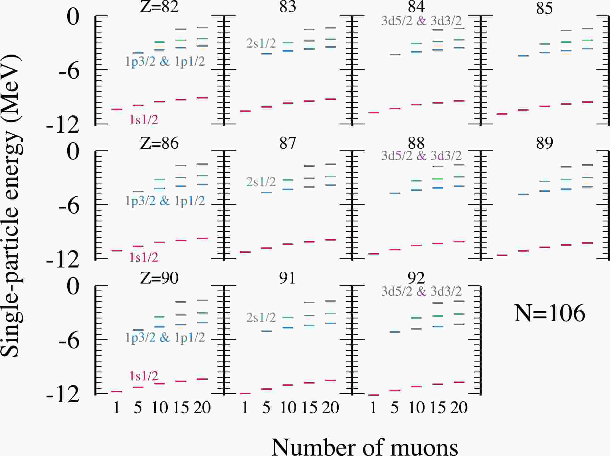
As shown in Fig. 1, we calculated the single-particle levels of muons for N=106 isotones (Z from 82 to 92). The red, blue, green, and purple lines represent
$ 1s_{1/2} $ ,$ 1p_{3/2} $ ($ 1p_{1/2} $ ),$ 2s_{1/2} $ , and$ 3d_{5/2} $ ($ 3d_{3/2} $ ) orbitals of muons, respectively. The$ 1p_{3/2} $ and$ 1p_{1/2} $ orbitals are degenerate given that the deformation is ignored, as are the$ 3d_{5/2} $ and$ 3d_{3/2} $ orbitals. We found that, for each nucleus, the muon single-particle energy level increases with the number of muons because more muons also lead to stronger repulsion among themselves. For example, the energy of the$ 1s_{1/2} $ orbital for$ Z = 82 $ goes from −10.39 MeV at$ N_\mu=1 $ to −9.10 MeV at$ N_\mu= 20 $ . For a certain number of muons, for instance, at$ N_\mu= 1 $ , the single-particle energy of$ 1s_{1/2} $ decreases monotonically with the increase in Z, that is, from$ -10.39 $ MeV at$ Z = 82 $ to$ -12.14 $ MeV at$ Z = 92 $ . For another example, at$ N_\mu= 10 $ , the energy level of muons$ 1s_{1/2} $ decreases gradually from −9.54 MeV at$ Z = 82 $ to$ -11.21 $ MeV at$ Z = 92 $ . The energy level of$ 1p_{3/2} $ decreases from −3.78 MeV to −4.79 MeV. The$ 2s_{1/2} $ energy level drops from −2.92 MeV to −3.60 MeV. This decreasing trend in energy levels holds true for other numbers of muons as well. Overall, as the number of protons increases, the single-particle energy levels of muons become slightly more negative. This can be attributed to the fact that more protons exert a stronger attractive force on the muons. There exists a large energy gap of approximately 6 MeV between the$ 1s_{1/2} $ orbital and the$ 1p_{3/2} $ ($ 1p_{1/2} $ ) orbital for the whole isotones.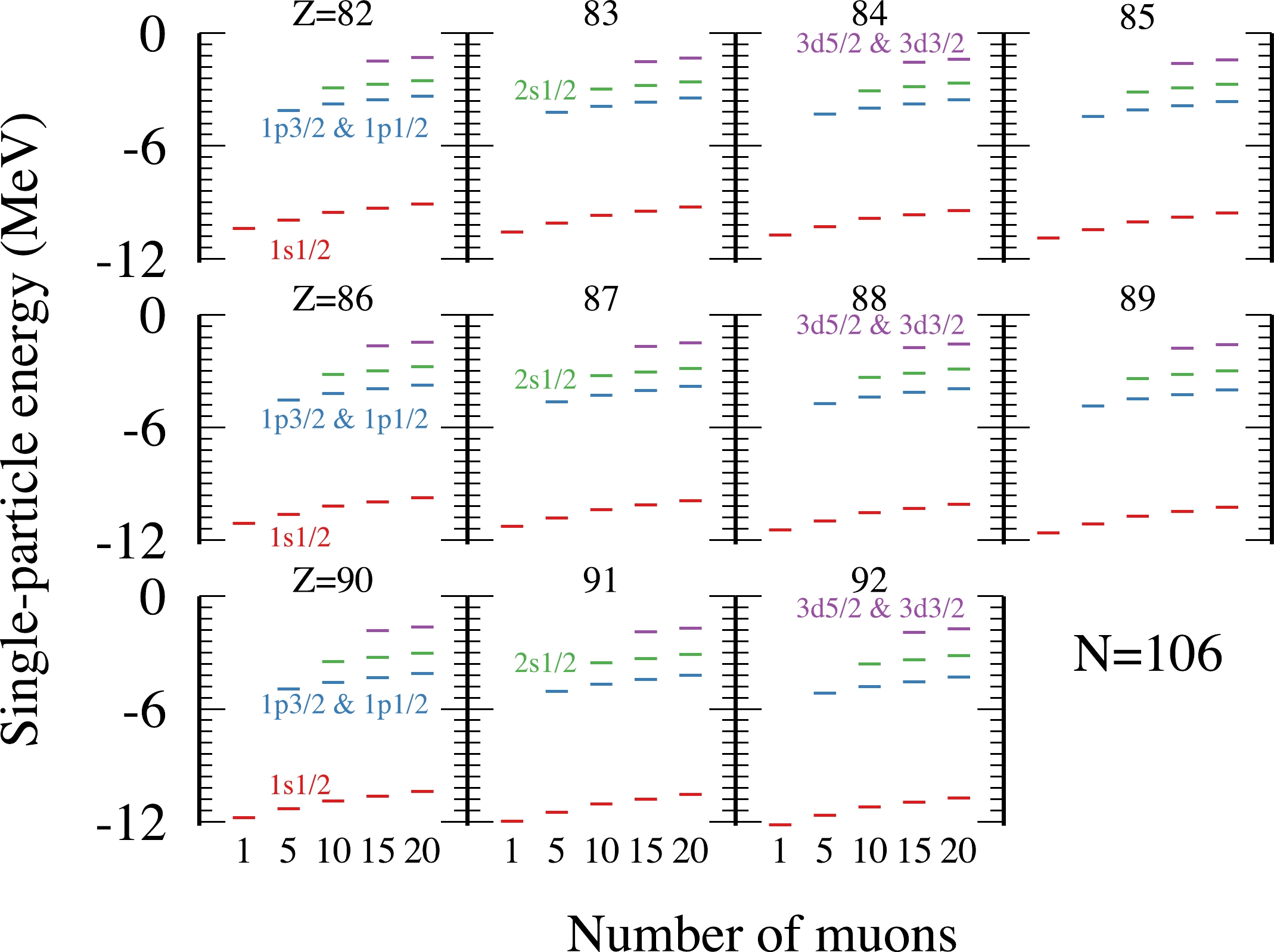
Figure 1. (color online) Single-particle levels of muons as a function of the number of muons for N=106 isotones (Z from 82 to 92). The red, blue, green, and purple lines represent
$ 1s_{1/2} $ ,$ 1p_{3/2} $ ($ 1p_{1/2} $ ),$ 2s_{1/2} $ , and$ 3d_{5/2} $ ($ 3d_{3/2} $ ) orbitals, respectively.We also calculated the single-particle levels of protons for different numbers of muons. Figure 2 shows the energy of the last single-particle level of protons as a function of the proton number for
$ N=106 $ isotones. The solid black, dashed red, dotted blue, dash-dot green, dash-dot-dot purple, and long dashed orange lines represent the numbers of muons 0, 1, 5, 10, 15, and 20, respectively. There is a clear energy gap between$ Z=82 $ and 83. Additionally, as the number of protons increases, the energy of the proton level becomes larger. Beyond proton number 87, the energy of the last energy level of the proton is greater than zero (at$ N_\mu=0 $ ). Interestingly, when muons are considered, the proton energy level can decrease significantly. The magnitude of the decrease enhances with the increase in the number of muons. Our calculations revealed that adding one muon can reduce the proton energy level by approximately 0.2 MeV, and 20 muons can reduce the proton energy level by approximately 1.7 MeV. Therefore, when muons are introduced, for nuclei with$ Z=87 $ , the last unbound energy level of the proton becomes a bound level. More muons mean more bound proton levels. After introducing 10 muons, the last proton energy levels for all$ N=106 $ isotones become bound single-particle states. Hence, introducing muons in experiments may enable the extrapolation of the proton drip line to obtain more proton-rich nuclei.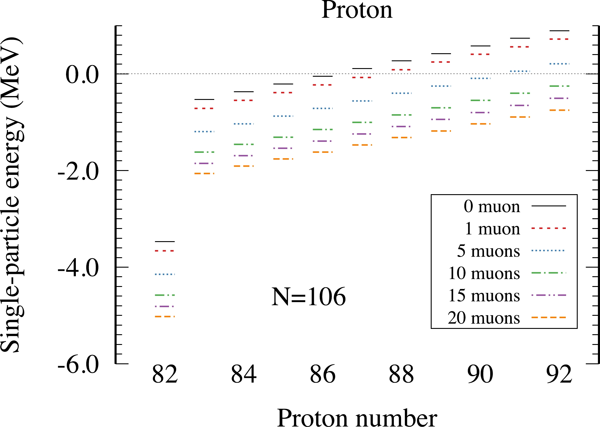
Figure 2. (color online) Energy of the last single-particle level of protons with different numbers of muons as a function of the proton number for N=106 isotones. The solid black, dashed red, dotted blue, dash-dot green, dash-dot-dot purple, and long dashed orange lines represent the number of muons 0, 1, 5, 10, 15, and 20, respectively.
The density distribution of muons with different numbers of them for
$ N=106 $ isotones is shown in Fig. 3. The dashed red, dotted blue, dash-dot green, dash-dot-dot purple, and long dashed orange lines represent the number of muons 1, 5, 10, 15, and 20, respectively. Although the density of muons diffuses to the space beyond 30 fm, the primary density is still distributed within 10 fm. Thus, there is considerable overlap with the nucleus. Simultaneously, as the number of protons increases, the center density of muons also enlarges by approximately$ 10 $ %, indicating that muons are attracted closer to the nucleus.
Figure 3. (color online) Density distribution of muons with different numbers of them for
$ N=106 $ isotones. The dashed red, dotted blue, dash-dot green, dash-dot-dot purple, and long dashed orange lines represent the number of muons 1, 5, 10, 15, and 20, respectively.Figure 4 shows the density distribution of protons with different numbers of muons for
$ N=106 $ isotones. The solid black, dashed red, dotted blue, dash-dot green, dash-dot-dot purple, and long dashed orange lines represent the number of muons 0, 1, 5, 10, 15, and 20, respectively. For the whole isotones, the density of protons is mainly distributed between 0 and 8 fm; consequently, there can be a significant overlap with the density of muons.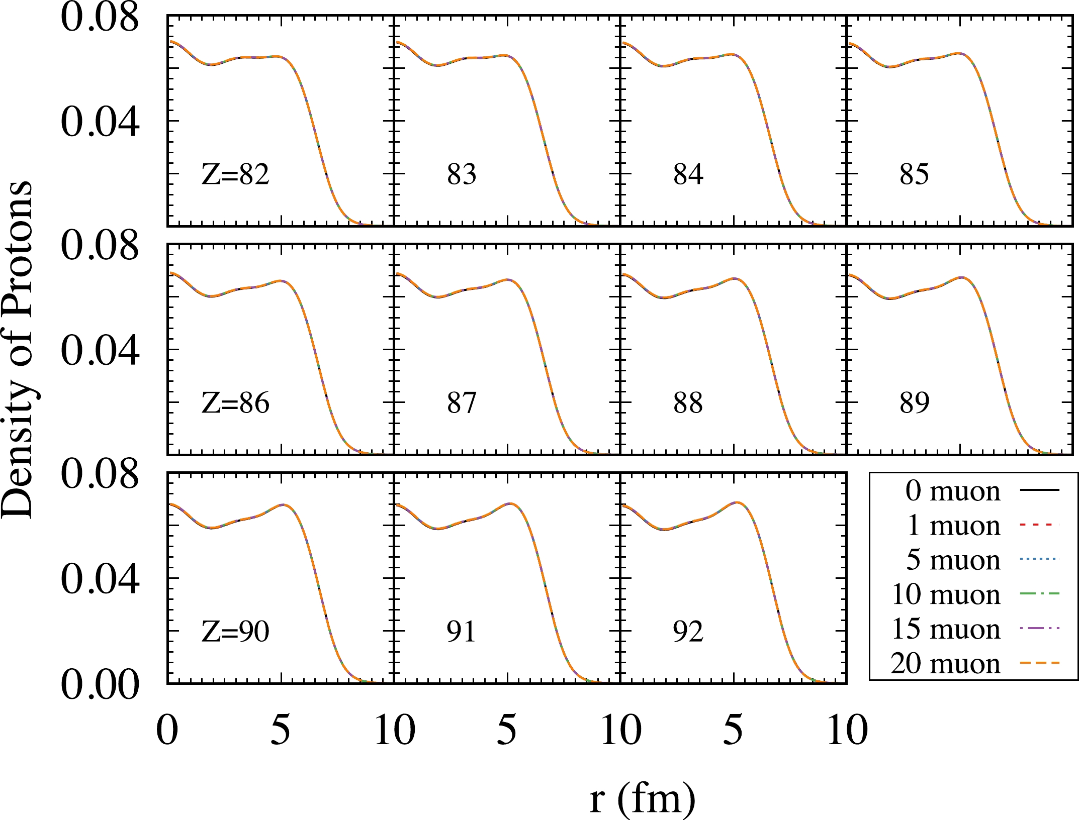
Figure 4. (color online) Density distribution of protons with different numbers of muons for
$ N=106 $ isotones. The solid black, dashed red, dotted blue, dash-dot green, dash-dot-dot purple, and long dashed orange lines represent the number of muons 0, 1, 5, 10, 15, and 20, respectively.To further study the influence of muons on the proton density, we zoomed in on the above plots. Figure 5 is the enlarged version of Fig. 4 in coordinate r from 0 to 5 fm. As discussed above, the proton center density varies by less than
$ 3 $ % across the isotones. The change in proton density due to different numbers of muons is minor, approximately$ 0.3 $ %.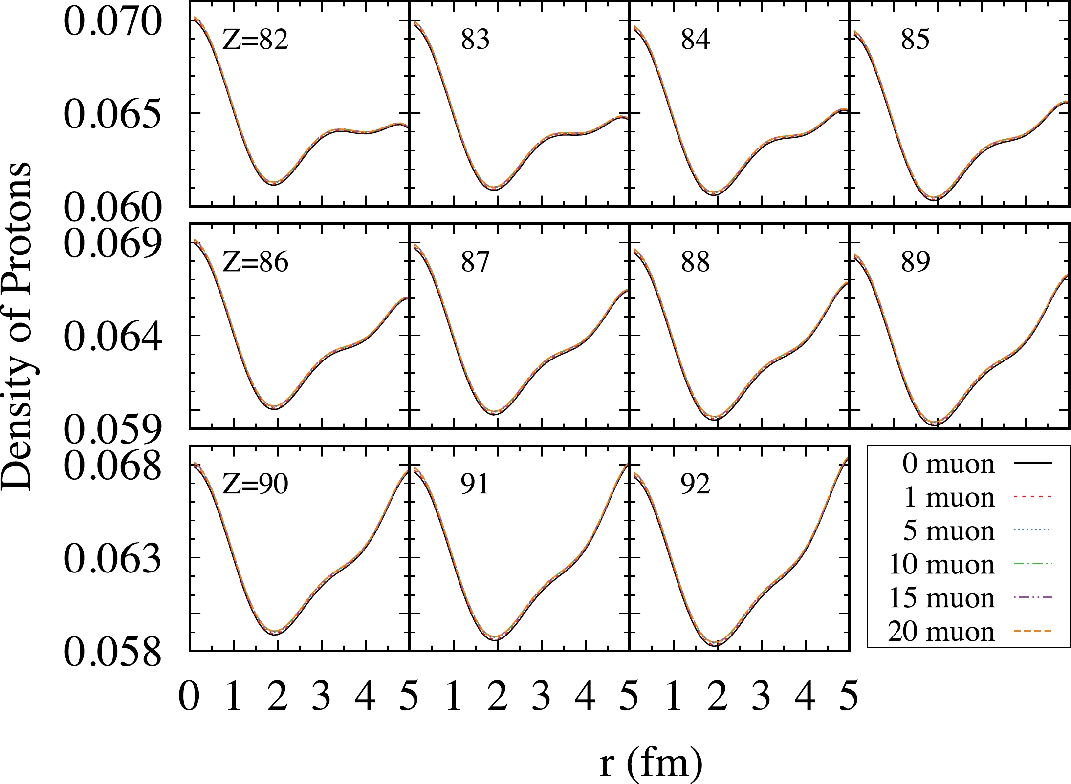
Figure 5. (color online) Same as Fig. 4 but enlarged in coordinate r from 0 to 5 fm.
The density distribution of neutrons with different numbers of muons for
$ N=106 $ isotones is presented in Fig. 6. Figure 7 is a partial enlargement of Fig. 6 from 0 to 5 fm. The solid black, dashed red, dotted blue, dash-dot green, dash-dot-dot purple, and long dashed orange lines represent the number of muons 0, 1, 5, 10, 15, and 20, respectively. The calculated neutron density is also mainly concentrated in the interval$ 0\sim 8 $ fm, which can overlap significantly with the muons density. However, compared to the case of protons, muons have a much weaker, almost negligible, effect on neutron density.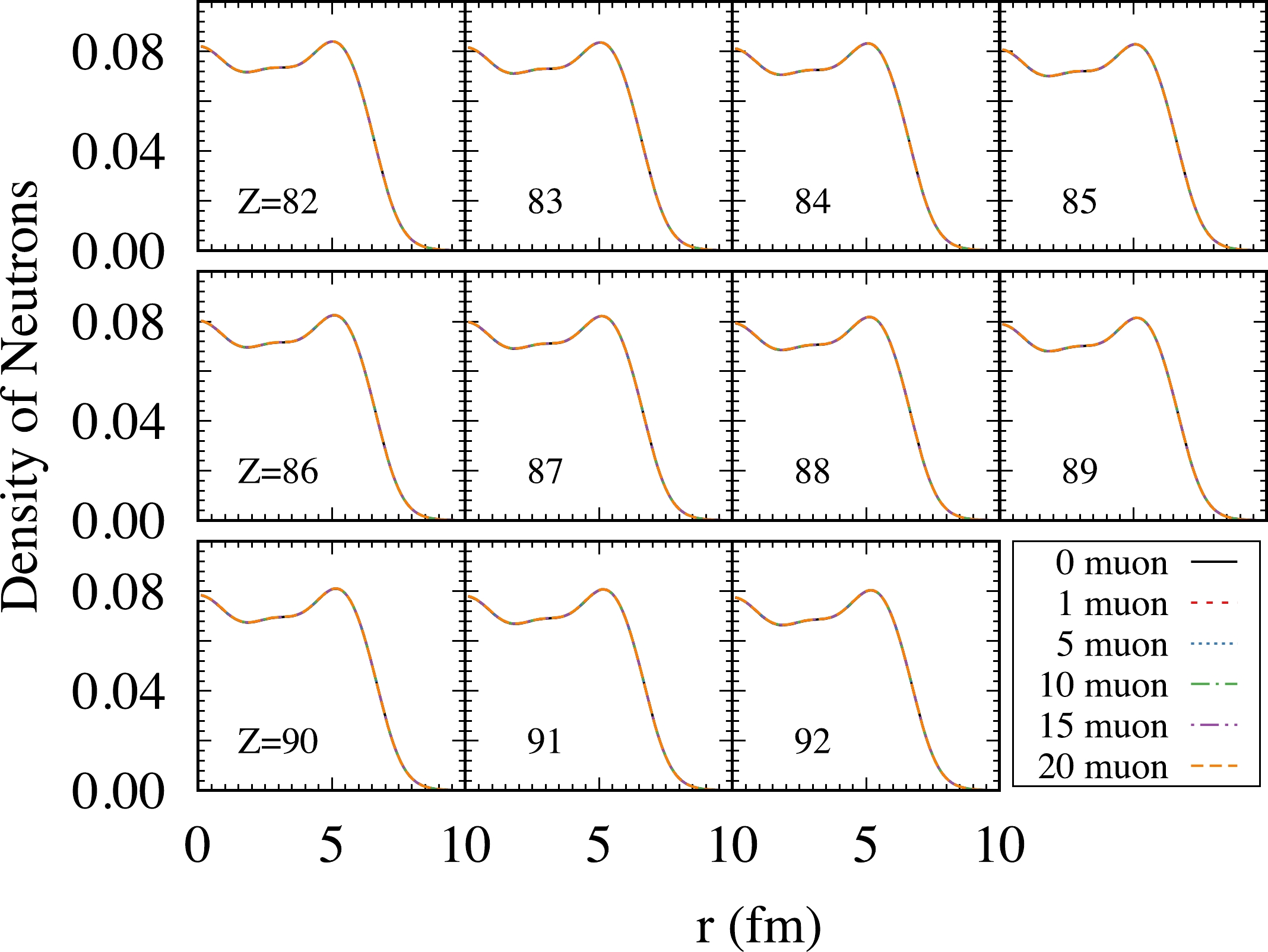
Figure 6. (color online) Density distribution of neutrons with different numbers of muons for
$ N=106 $ isotones. The solid black, dashed red, dotted blue, dash-dot green, dash-dot-dot purple, and long dashed orange lines represent the number of muons 0, 1, 5, 10, 15, and 20, respectively.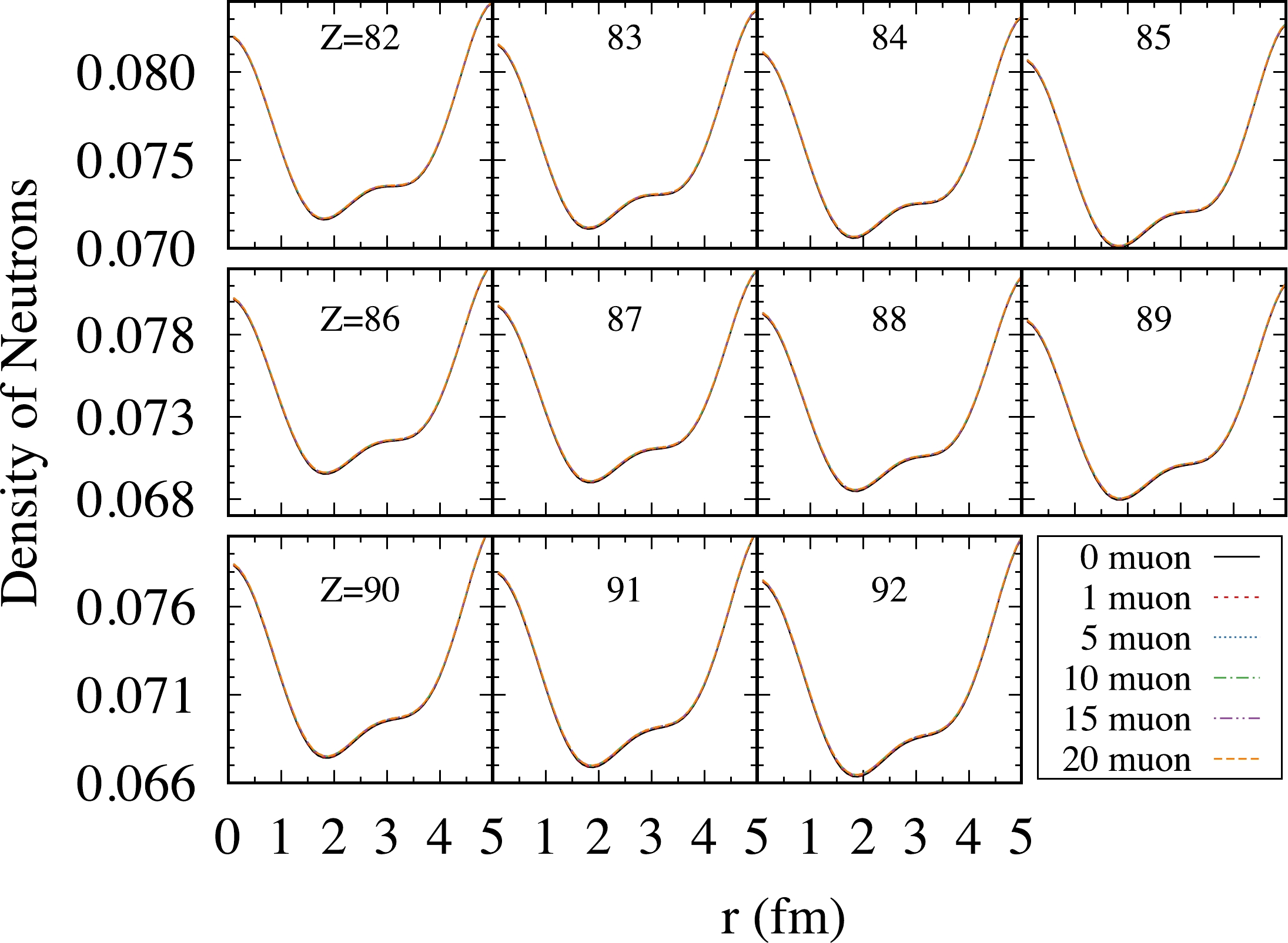
Figure 7. (color online) Same as Fig. 6 but enlarged in coordinate r from 0 to 5 fm.
Figure 8 shows the Coulomb potential generated by
$ \rho_{\mu} $ with different numbers of muons for$ N=106 $ isotones. The dashed red, dotted blue, dash-dot green, dash-dot-dot purple, and long dashed orange lines represent the number of muons 1, 5, 10, 15, and 20, respectively (the Coulomb potential is calculated from Eq. (8) by substituting into the muon density). Although the muon is negatively charged, here we take its absolute value. We found that the Coulomb potential of the muons increases by approximately$ 3.5 $ % as the number of protons increases from 82 to 92. However, for a particular nucleus, increasing the number of muons from 1 to 20 increases the Coulomb potential of the muons by approximately 1.5 MeV. For example, for a nucleus with$ Z=87 $ , the Coulomb potential of muons near the center, corresponding to number of muons 1, 5, 10, 15, and 20, is 0.2, 0.8, 1.3, 1.5, and 1.7 MeV, which is approximately the same as the change in energy of the proton Fermi level.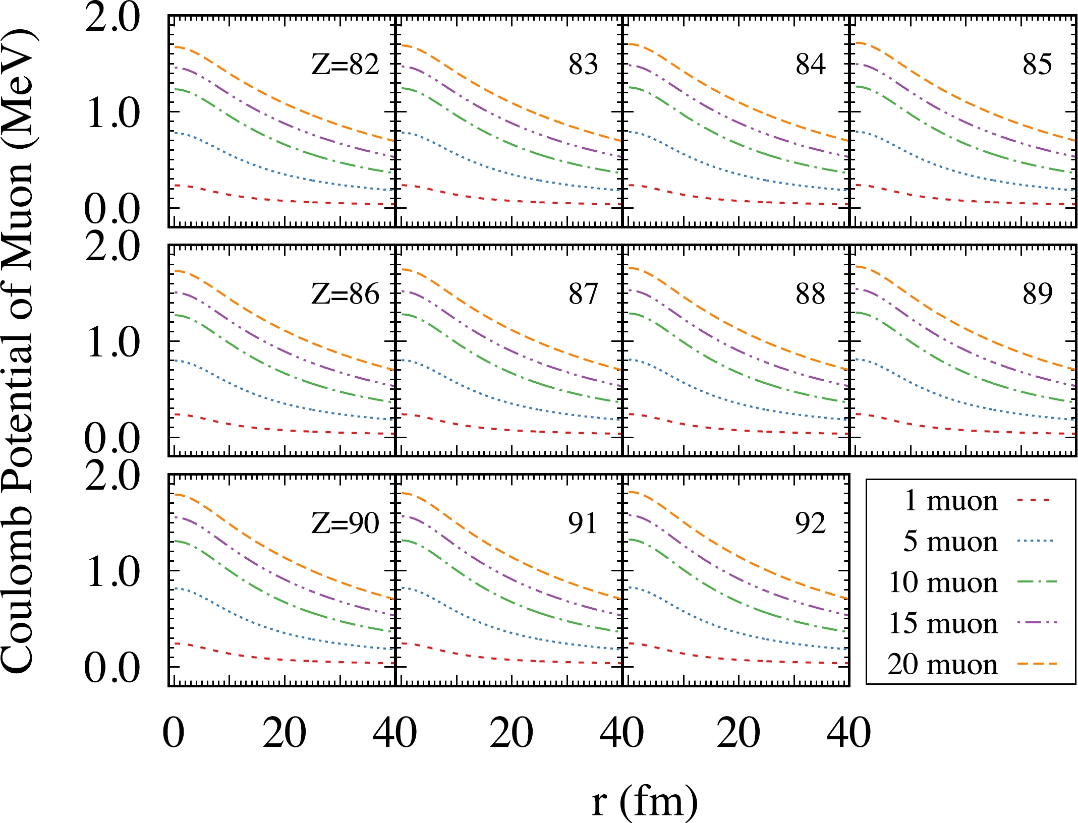
Figure 8. (color online) Coulomb potential generated by
$ \rho_{\mu} $ with different numbers of muons for$ N=106 $ isotones. The dashed red, dotted blue, dash-dot green, dash-dot-dot purple, and long dashed orange lines represent the number of muons 1, 5, 10, 15, and 20, respectively. Here, the absolute value of the Coulomb potential is taken.The Coulomb potential generated by
$ \rho_{\rm p} $ with different numbers of muons for$ N=106 $ isotones is shown in Fig. 9. The inserts are enlarged plots in coordinate r from 0 to 1 fm. The solid black, dashed red, dotted blue, dash-dot green, dash-dot-dot purple, and long dashed orange lines represent the number of muons 0, 1, 5, 10, 15, and 20, respectively. We found that as Z increases from 82 to 92, the Coulomb potential of the protons increases by approximately$ 8 $ %. However, for a particular nucleus, increasing$ N_\mu $ from 1 to 20 changes the Coulomb potential of the proton by less than$ 0.1 $ %.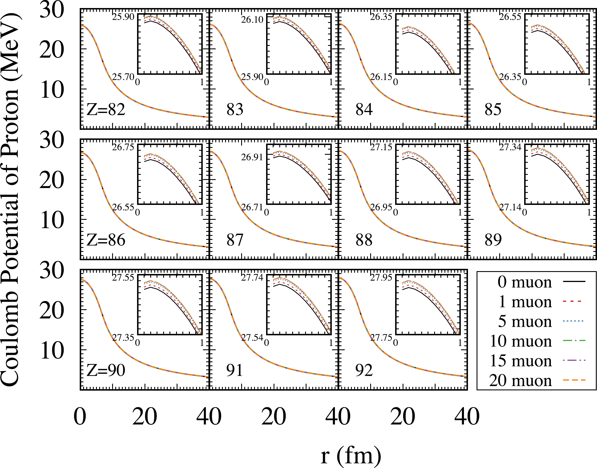
Figure 9. (color online) Coulomb potential generated by
$ \rho_{\rm p} $ with different numbers of muons for$ N=106 $ isotones. The solid black, dashed red, dotted blue, dash-dot green, dash-dot-dot purple, and long dashed orange lines represent the number of muons 0, 1, 5, 10, 15, and 20, respectively. Inserts: enlarged subfigure in coordinate r from 0 to 1 fm. -
In this study, we analyzed the properties of the nucleus in muon atoms utilizing a spherical mean-field calculation with Skyrme interaction. Taking
$ N=106 $ isotones as an example, we investigated the influence of the muons on the nuclear structure. It was found that the single-particle levels of muons decrease with the increase in the number of protons and rise with the increase in the number of muons. More importantly, we found that, although the proton Fermi level changes from bound to unbound with the increase in Z, the addition of muons significantly reduces the Fermi level of the proton. Moreover, increasing the muons from 0 to 20 even lowers the proton Fermi level by 1.7 MeV. This could allow for the expansion of the proton dripline on the nuclear chart and the production of a nucleus with a value of Z of approximately 120. We analyzed the effect of muons on the proton and neutron density distribution. We found that the neutron density is hardly affected by muons, while the proton density changes by approximately 0.3% in the range of 0 to 5 fm due to the influence of muons. Additionally, the Coulomb potential caused by the protons changes by approximately 0.1% due to the influence of muons. However, the Coulomb potential generated by muons can provide energies ranging from 0.2 to 1.7 MeV inside the nucleus, and this order of magnitude is roughly equivalent to the drop in energy of the proton Fermi level.
Expanding proton dripline by employing a number of muons
- Received Date: 2023-07-05
- Available Online: 2023-11-15
Abstract: Through mean-field calculations, we demonstrate that, in a large Z nucleus binding multiple muons, these heavy leptons localize within a few dozen femtometers of the nucleus. The mutual Coulomb interactions between the muons and protons can lead to a substantial decrease in proton chemical potential, surpassing 1 MeV. These findings imply that, in principle, the proton-dripline can be expanded on the nuclear chart, suggesting the possible production of nuclei with Z around 120.


 DownLoad: