


 Abstract
 HTML
HTML Reference
 Related
 PDF
PDF


-
In quantum electrodynamics, the Schwinger effect, a striking manifestation of the nontrivial structure of the quantum vacuum, materializes virtual electron-positron pairs into real particles under the influence of a potent external electromagnetic field. Schwinger conducted a detailed study on this phenomenon in 1951, wherein he calculated the production rate Γ under the condition of a weak coupling and weak field [1]. Affleck-Alvarez-Manton (AAM) subsequently calculated it just using a weak-field approximation [2], obtaining the following result
$ \begin{equation} \Gamma\sim {\rm exp}\Bigg{(}{\frac{-\pi m^2}{eE}+\frac{e^2}{4}}\Bigg{)}. \end{equation} $

(1) Here, the created particles’ mass and charge are denoted by m and e, respectively. E is the external electric field. Far from being unique to QED, the Schwinger effect is a pervasive phenomenon for various quantum field theories coupled to an abelian gauge field. Nevertheless, the Schwinger effect is typically non-perturbative because it requires an extremely strong electric field to be significant, making it challenging to evaluate within the framework of quantum field theory. To address this challenge, the use of holography, specifically the AdS/CFT correspondence – a potent link between quantum gravity in a higher-dimensional anti-de Sitter space and conformal field theory on its boundary – presents a promising alternative approach, making the evaluation of the Schwinger effect within this framework particularly compelling [3−5]. Semenoff and Zarembo studied the pair creation in the
$ \mathcal N=4 $ supersymmetric Yang-Mills (SYM) theory, which is dual to a probe D3-brane placed at an intermediate position in the bulk and found [6]$ \begin{equation} \Gamma\sim {\rm exp}\Bigg{[}-\frac{\sqrt{\lambda}}{2}\Bigg{(}\sqrt{\frac{E_c}{E}}-\sqrt{\frac{E}{E_c}}\Bigg{)}^2\Bigg{]}, \end{equation} $

(2) with
$ \begin{equation} E_c=\frac{2\pi m^2}{\sqrt{\lambda}}, \end{equation} $

(3) where the value of the critical field
$ E_c $ is consistent with the DBI results. Inspired by Semenoff and Zarambo’s work, numerous efforts have been made in this direction to study the Schwinger effect. In Ref. [7], the universal aspects of a holographic Schwinger effect were considered in general backgrounds. The holographic Schwinger effect in some AdS/QCD models was studied [8, 9]. The pair production in a confining D3-brane background with chemical potential was investigated in [10]. The potential analysis of the holographic Schwinger effect in a magnetized background was conducted in [11]. Other important works can be found in [12−20].Anisotropy refers to the distinct characteristics exhibited by certain directions or dimensions in a medium or spacetime, which can arise from diverse sources including magnetic fields, rotation, deformation, or phase transitions. It plays a crucial role in various systems, ranging from condensed matter physics to cosmology, and it is important when capturing the behavior of realistic systems such as quark-gluon plasma (QGP) or condensed matter systems that deviate from isotropy or homogeneity. One motivation for this work comes from the experiments showing that the QGP created in an ultra relativistic heavy ion collision is locally anisotropic in its early stages as the system expands predominantly in the direction of the collision axis [21, 22]. Mateos and Trancanelli have made significant progress in the study of anisotropy by developing a IIB supergravity solution dual to a spatially anisotropic
$ \mathcal N=4 $ SYM plasma [23, 24]. In Refs. [25−27], the static potential, the drag force, and the jet quenching parameter in anisotropic plasma were discussed. Further research in this area can be found in [28−32]. In RHIC and LHC experiments, heavy ion collisions produce strong electromagnetic fields as well as anisotropy; therefore, it is interesting to study the impact of this anisotropy on the Schwinger effect, with promising prospects for its observation in the future.In addition to anisotropy, given the close connection between the holographic Schwinger effect and string theory, we seek to investigate the Schwinger effect with higher curvature corrections, which naturally arise in the low-energy effective action of heterotic string theory. Here, we focus on the Gauss-Bonnet term, a leading correction to Einstein gravity that preserves the ghost-free property of the field equations [33]. In Refs. [19, 20], the authors studied the holographic Schwinger effect with the Gauss-Bonnet term. Extending prior work, we investigate the influence of both anisotropy and the Gauss-Bonnet coupling on the Schwinger effect, as their combined influence is yet to be studied.
In this study, we focus on the holographic Schwinger effect in the 5-dimensional AdS-axion-dilaton system with a Gauss-Bonnet term and anisotropy adopted using an axion field. Our goal is to investigate how anisotropy and the Gauss-Bonnet coupling affect the Schwinger effect at a qualitative level. Our paper is organized as follows. In the next section, we introduce the 5-dimensional AdS-axion-dilaton system with a Gauss-Bonnet term, which was proposed in [34]. In Sec. III, we perform a potential analysis considering the anisotropic background metric and focus on the effects of anisotropy. In Sec. IV, we analyze the impact of the Gauss-Bonnet coupling on the Schwinger effect and the critical electric field. A summary and discussion are presented in the final section.
-
The 5-dimensional AdS-axion-dilaton gravity action with a Gauss-Bonnet term is given by [34]
$ \begin{aligned}[b] S=&\frac{1}{16 \pi G} \int {\rm d}^5 x \sqrt{-g}\Bigg[R+\frac{12}{\tilde{\ell}^2}-\frac{1}{2}(\partial \phi)^2-\frac{{\rm e}^{2 \phi}}{2}(\partial \chi)^2\\&+\frac{\tilde{\ell}^2}{2} \lambda_{\mathrm{GB}} \mathcal{L}_{\mathrm{GB}}\Bigg]+S_{\mathrm{GH}}, \end{aligned} $

(4) where ϕ and χ are the dilaton and axion scalar fields, respectively.
$\lambda_{\rm GB}$ is the Gauss-Bonnet coupling and$ \begin{equation} \mathcal{L}_{\mathrm{GB}}=R^2-4 R_{m n} R^{m n}+R_{m n r s} R^{m n r s} \end{equation} $

(5) is the Gauss-Bonnet term. The range of
$\lambda_{\rm GB}$ is$-\dfrac{7}{36} < \lambda_{\rm GB}\leq\dfrac{9}{100}$ , where the lower bound ensures a positive-definite boundary energy density and the upper bound prevents causality violation at the boundary [35].$ \tilde{\ell} $ is a parameter with dimensions of length, and we set it to one. To have a well-defined variational problem, we include a surface term denoted by$ S_{\mathrm{GH}} $ . As discussed in [36], the metric of the black brane solution takes the form$ \begin{aligned}[b] {\rm d} s^2=&G_{m n} {\rm d} x^m {\rm d} x^n=\frac{1}{u^2}\Bigg(-F(u) B(u) {\rm d} t^2+{\rm d} x^2\\&+{\rm d} y^2+H(u) {\rm d} z^2+\frac{{\rm d} u^2}{F(u)}\Bigg), \end{aligned} $

(6) with
$ \begin{equation} \chi=a z, \quad \phi=\phi(u), \end{equation} $

(7) where u is the radial coordinate describing the 5th dimension.
$ u=u_{\mathrm{H}} $ is the event horizon and$ u=0 $ is the boundary. The axion field introduces spatial anisotropy in the z-direction controlled by the anisotropy parameter a. Here, the axion field with the form$ \chi=a z $ is dual to the SYM theory deformed by a θ-parameter,$ \theta=2 \pi n z $ , z denotes the spatial coordinate, and n is the number density of$ D 7 $ number per unit length with dimensions of energy; this deformation breaks isotropy and acts as an anisotropic external source [24]. Limited to cases with small anisotropy, we are able to obtain analytical solutions to the dilaton field ϕ and the metric components F, B, and H at order$ O\left(a^2\right) $ , as described in [36]$ \begin{aligned}[b] \phi(u) &=a^2 \phi_2(u)+O\left(a^4\right), \quad\quad F(u) =F_0(u)+a^2 F_2(u)+O\left(a^4\right), \\ B(u) &=B_0\left(1+a^2 B_2(u)+O\left(a^4\right)\right),\quad\quad H(u) =1+a^2 H_2(u)+O\left(a^4\right), \end{aligned} $

(8) with
$ \begin{equation} F_0(u)=\frac{1}{2 \lambda_{\mathrm{GB}}}\left(1-\sqrt{1-4 \lambda_{\mathrm{GB}}\left(1-\frac{u^4}{u_{\mathrm{H}}^4}\right)}\right), \quad B_0=\frac{1+\sqrt{1-4 \lambda_{\mathrm{GB}}}}{2} , \end{equation} $

(9) $ \begin{aligned}[b] &\phi_2(u)=\frac{1}{8} u_{\mathrm{H}}^2\left(\log \alpha(u)+U_0-U(u)\right), \\ &F_2(u)=\frac{u^4}{12 U_0^2 u_{\mathrm{H}}^2 U(u)}\left(-\log \left(\frac{\alpha(u)}{\alpha\left(u_{\mathrm{H}}\right)}\right)-\frac{6 u^4 \lambda_{\mathrm{GB}}}{u_{\mathrm{H}}^4}+\frac{4 u^2 \lambda_{\mathrm{GB}}}{u_{\mathrm{H}}^2}+\frac{U_0^2 u_{\mathrm{H}}^2}{u^2}+6 \lambda_{\mathrm{GB}}+U(u)-2\right), \\ &B_2(u)=\frac{u^2 u_{\mathrm{H}}^2}{24 U_0^2\left(u_{\mathrm{H}}^2+u^2\right)}\left(-\frac{6 u^4 \lambda_{\mathrm{GB}}}{u_{\mathrm{H}}^4}-\frac{2 u^2 \lambda_{\mathrm{GB}}}{u_{\mathrm{H}}^2}+4 \lambda_{\mathrm{GB}}-\frac{8 \phi_2(u)}{u_{\mathrm{H}}^2}-\frac{8 \phi_2(u)}{u^2}-2 U(u)-2\right), \\ &H_2(u)=\frac{u_{\mathrm{H}}^2}{8 U_0^2}\left(-\log \alpha(u)+2 \lambda_{\mathrm{GB}} \frac{u^2}{u_{\mathrm{H}}^2}\left(\frac{u^2}{u_{\mathrm{H}}^2}-2\right)+U(u)-U_0\right), \end{aligned} $

(10) and
$ \begin{equation} \alpha(u)=\left(\frac{2 u^2 \sqrt{\lambda_{\mathrm{GB}}}+u_{\mathrm{H}}^2 U(u)}{U_0 u_{\mathrm{H}}^2}\right)^{2 \sqrt{\lambda_{\mathrm{GB}}}} \frac{\left(-4 \lambda_{\mathrm{GB}} u_{\mathrm{H}}^2\left(u_{\mathrm{H}}^2+u^2\right)+u_{\mathrm{H}}^4 U(u)+u_{\mathrm{H}}^4\right)}{\left(2 B_0-4 \lambda_{\mathrm{GB}}\right)\left(u_{\mathrm{H}}^2+u^2\right)^2} , \end{equation} $

(11) $ \begin{equation} U(u) \equiv \sqrt{1-4 \lambda_{\mathrm{GB}}\left(1-\frac{u^4}{u_{\mathrm{H}}^4}\right)}, U_0 \equiv U(0). \end{equation} $

(12) Then, the temperature can be given as
$ \begin{equation} T=\sqrt{B_0}\left(\frac{1}{\pi u_{\mathrm{H}}}-\frac{2 B_0-6 \lambda_{\mathrm{GB}}+\sqrt{\lambda_{\mathrm{GB}}} \log \left(\dfrac{1+2 \sqrt{\lambda_{\mathrm{GB}}}}{1-2 \sqrt{\lambda_{\mathrm{GB}}}}\right)-\log \left(\dfrac{4 B_0}{\sqrt{1-4 \lambda_{\mathrm{GB}}}}\right)}{48 \pi\left(1-4 \lambda_{\mathrm{GB}}\right)} u_{\mathrm{H}} a^2+O\left(a^4\right)\right). \end{equation} $

(13) -
As the background geometry is anisotropic, it is reasonable to consider the test particle pair to be perpendicular (denoted by “
$ \perp $ ”) to and parallel (denoted by “$ \parallel $ ”) to the direction of anisotropy.First, we study the test particle pair along the direction transversal to the anisotropy. In this case, the coordinates are parameterized by
$ \begin{equation} t=\tau, \quad x=\sigma, \quad y=z=0, \quad u=u(\sigma). \end{equation} $

(14) The classical string action can reduce to the Nambu-Goto action
$ \begin{equation} S=T_F \int {\rm d} \sigma {\rm d} \tau \mathcal{L}=T_F \int {\rm d} \sigma {\rm d} \tau \sqrt{\operatorname{det} g_{\alpha \beta}}\ , \end{equation} $

(15) where
$ T_F=\dfrac{1}{2\pi\alpha^\prime} $ is the string tension and$ g_{\alpha\beta} $ is the induced metric on the string world sheet embedded in the target space. Then, the lagrangian density is found to be$ \begin{equation} \mathcal{L}=\sqrt{\operatorname{det} g_{\alpha \beta}}=\frac{1}{u^2} \sqrt{ F(u) B(u)+B(u) \dot{u}^2}. \end{equation} $

(16) Note that the action does not depend on σ explicitly; therefore, the corresponding Hamiltonian is a constant, that is
$ \begin{equation} H=\mathcal{L}-\frac{\partial \mathcal{L}}{\partial \dot{u}} \dot{u}=\text { Constant }. \end{equation} $

(17) Considering the boundary condition
$ \begin{equation} \dot{u}=\frac{{\rm d} u}{{\rm d} \sigma}=0, \quad u=u_c\left(u_0<u_c<u_h\right), \end{equation} $

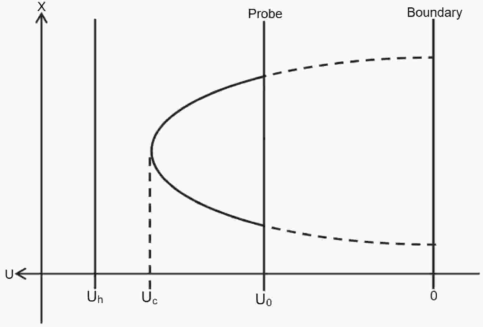
(18) where the probe D3-brane is located at an intermediate position (
$ u=u_0 $ ) between the horizon and the boundary. The configuration of the string world sheet is depicted in Fig. 1. Then, a differential equation is derived
Figure 1. String configuration.
$ \begin{equation} \dot{u}=\frac{{\rm d} u}{{\rm d} \sigma}=\frac{\sqrt{F(u)} \sqrt{-B(u_c) F(u_c) u^4+B(u) F(u) u_c^4}}{u^2 \sqrt{B(u_c)F(u_c)} }. \end{equation} $

(19) By integrating this expression, the separation length
$ x_\perp $ of the particle pair when perpendicular to the anisotropy can be written as$ \begin{equation} x_{\perp}=2 \int_{u_0}^{u_c} {\rm d} u \frac{u^2 \sqrt{B(u_c)F(u_c)} }{\sqrt{F(u)} \sqrt{-B(u_c) F(u_c) u^4+B(u) F(u) u_c^4}}. \end{equation} $

(20) The sum of potential energy (PE) and static energy (SE) of the string is given by
$ \begin{equation} V_{(C P+{\rm S E})(\perp)}=2 T_F \int_{u_0}^{u_c} {\rm d} u \frac{B(u) u_c^2 \sqrt{F(u)}}{u^2 \sqrt{-B(u_c) F(u_c) u^4+B(u) F(u) u_c^4}}. \end{equation} $

(21) The next task is to calculate the test particle pair parallel to the anisotropy. The coordinates are parameterized by
$ \begin{equation} t=\tau, \quad z=\sigma, \quad x=y=0, \quad u=u(\sigma). \end{equation} $

(22) By repeating the previous calculation, the separation length
$ x_\parallel $ of the particle pair when parallel to the anisotropy is$ \begin{aligned}[b] x_{\parallel}=&2 \int_{u_0}^{u_c} {\rm d} u\\&\times \frac{u^2 \sqrt{B(u_c) F(u_c) H(u_c)} }{\sqrt{F(u) H(u)} \sqrt{-B(u_c) F(u_c) H(u_c) u^4 + B(u) F(u) H(u) u_c^4}}. \end{aligned} $

(23) The sum of PE and SE in the parallel case is
$ \begin{aligned}[b] V_{(C P+{\rm S E})(\parallel)}=&2 T_F \int_{u_0}^{u_c} {\rm d} u \\&\times\frac{B(u) u_c^2 \sqrt{F(u) H(u)}}{u^2 \sqrt{-B(u_c) F(u_c) H(u_c)u^4+B(u) F(u) H(u) u_c^4}}. \end{aligned} $

(24) Next, we calculate the critical electric field
$ E_c $ . The DBI action is given by$ \begin{equation} S_{\rm D B I}=-T_{D 3} \int {\rm d}^4 x \sqrt{-\operatorname{det}\left(G_{\mu \nu}+\mathcal{F}_{\mu \nu}\right)}, \quad T_{D 3}=\frac{1}{g_s(2 \pi)^3 \alpha^{\prime^2}}, \end{equation} $

(25) where
$ T_{D3} $ is the D3-brane tension. First, we consider the electric field perpendicular to the anisotropic direction. We can then find$ \begin{equation} G_{\mu \nu}+\mathcal{F}_{\mu \nu}=\left(\begin{array}{cccc} -\dfrac{B(u) F(u)}{u^2} & 2 \pi \alpha^{\prime} E_\perp & 0 & 0 \\ -2 \pi \alpha^{\prime} E_\perp & \dfrac{1}{u^2} & 0 & 0 \\ 0 & 0 & \dfrac{1}{u^2} & 0 \\ 0 & 0 & 0 & \dfrac{H(u)}{u^2} \end{array}\right), \end{equation} $

(26) which leads to
$ \begin{equation} \operatorname{det}\left(G_{\mu \nu}+\mathcal{F}_{\mu \nu}\right)=\frac{H(u)}{u^8} (-B(u) F(u) + 4 E_\perp^2 \pi^2 u^4 \alpha^2). \end{equation} $

(27) Plugging (27) into (25) and making the probe D3-brane located at
$ u=u_0 $ , we get$ \begin{equation} S_{\rm D B I}=-T_{D 3} \int {\rm d}^4 x \sqrt{-\frac{H(u_0)}{u_0^8} (-B(u_0) F(u_0) + 4 E_\perp^2 \pi^2 u_0^4 \alpha^2)}. \end{equation} $

(28) The quantity under the square root of (28) should be non-negative. Thus, we require
$ \begin{equation} -\frac{H(u_0)}{u_0^8} (-B(u_0) F(u_0) + 4 E_\perp^2 \pi^2 u_0^4 \alpha^2) \ge 0. \end{equation} $

(29) As a result, the critical field is obtained by
$ \begin{equation} E_{c(\perp)}=T_F \sqrt{\frac{B(u_0) F(u_0)}{u_0^4}}. \end{equation} $

(30) Using the same method, the critical field when the electric field is parallel to the anisotropy can be found
$ \begin{equation} E_{c(\parallel)}=T_F \sqrt{\frac{B(u_0) F(u_0) H(u_0)}{u_0^4}}. \end{equation} $

(31) For convenience, we introduce a dimensionless parameter
$ \begin{equation} \alpha\equiv\frac{E}{E_c}. \end{equation} $

(32) When the particle pair and the electric field are perpendicular to the anisotropy, the total potential
$V_{{\rm tot}(\perp)}$ of the pair can be written as$ \begin{aligned}[b] V_{{\rm tot}(\perp)} &=V_{(C P+{\rm SE})(\perp)}-E_\perp x_{\perp} \\ &=V_{(C P+{\rm SE})(\perp)}-\alpha E_{c(\perp)} x_{\perp} . \end{aligned} $

(33) When the pair and the electric field are parallel to the anisotropy, the total potential
$ V_{\rm tot(\parallel)} $ of the pair will be$ \begin{aligned}[b] V_{\text {tot }(\parallel)} &=V_{(C P+{\rm SE})(\parallel)}-E_\parallel x_{\parallel} \\ &=V_{(C P+{\rm SE})(\parallel)}-\alpha E_{c(\parallel)} x_{\parallel} . \end{aligned} $

(34) In this section, we mainly focus on the effect of the anisotropy on the separation length, the total potential, and the critical field. We now discuss the numerical results. Fig. 2 shows the correlation between the separation length x and
$ u_c $ for different anisotropy parameters. The results of Fig. 2 reveal that the presence of anisotropy decreases the maximum value of the separation length. Furthermore, it seems that the separation length varies more markedly in the direction of the pair parallel to the anisotropy compared to the transverse case.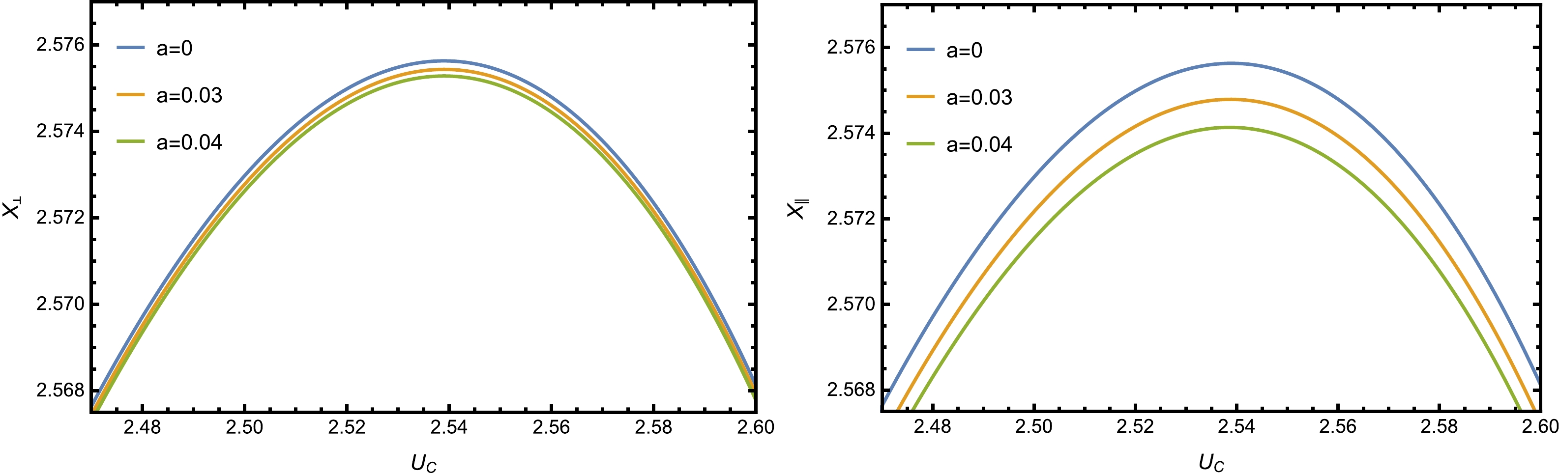
Figure 2. (color online) Separation length x versus
$ u_c $ when$T=0.1 ~{\rm GeV}$ and$\lambda_{\rm GB}=0.01$ . Left: The pair is perpendicular to the anisotropy. Right: The pair is parallel to the anisotropy.In Fig. 3, we plot the total potential
$V_{\rm tot}$ as a function of the separation length x for different values of α when$T=0.1 ~{\rm GeV}$ ,$a=0.03 ~{\rm GeV}$ , and$\lambda_{\rm GB}=0.01$ . In both cases, we can find that when$ \alpha < 1 \; (E < E_c) $ , the potential barrier is present and the Schwinger effect can be explained as a tunneling process. When$ \alpha = 1 \; (E = E_c) $ , the potential barrier vanishes and there is no suppression of the Schwinger effect. When$ \alpha > 1 \; (E > E_c) $ , the pair production is catastrophic and the vacuum becomes unstable. The results of above analysis are consistent with those reported in [37].
Figure 3. (color online) Total potential
$V_{\rm tot}$ as a function of the separation length x for different values of α when$T=0.1 ~{\rm GeV}$ ,$a=0.03 ~{\rm GeV}$ , and$\lambda_{\rm GB}=0.01$ . Left: The pair and the electric field are perpendicular to the anisotropy. Right: The pair and the electric field are parallel to the anisotropy.To demonstrate the effect of anisotropy on the potential barrier, in Fig. 4 we fix
$ \alpha = 0.6 $ and plot the total potential$V_{\rm tot}$ versus x when the particle pair and the electric field are perpendicular to the anisotropy as well as when they are parallel to the anisotropy. From the left panel of Fig. 4, we can see that for a fixed α, an increase in the anisotropy parameter a leads to a decrease in the height and width of the barrier. It is known that a higher potential barrier makes it more difficult for the produced pair to escape to infinity. Therefore, the presence of anisotropy tends to increase the Schwinger effect when the particle pair and the electric field are perpendicular to the anisotropy. From the right panel of Fig. 4, we can find that the anisotropy increases the height and width of the potential barrier, which weakens the Schwinger effect when the pair and the electric field are parallel to the anisotropy. The above results are in qualitative agreement with the findings of [31, 32]. It should be noted that the potential barrier is more visibly affected by the anisotropy in the parallel case because the anisotropy parameter has a greater influence on the anisotropic direction.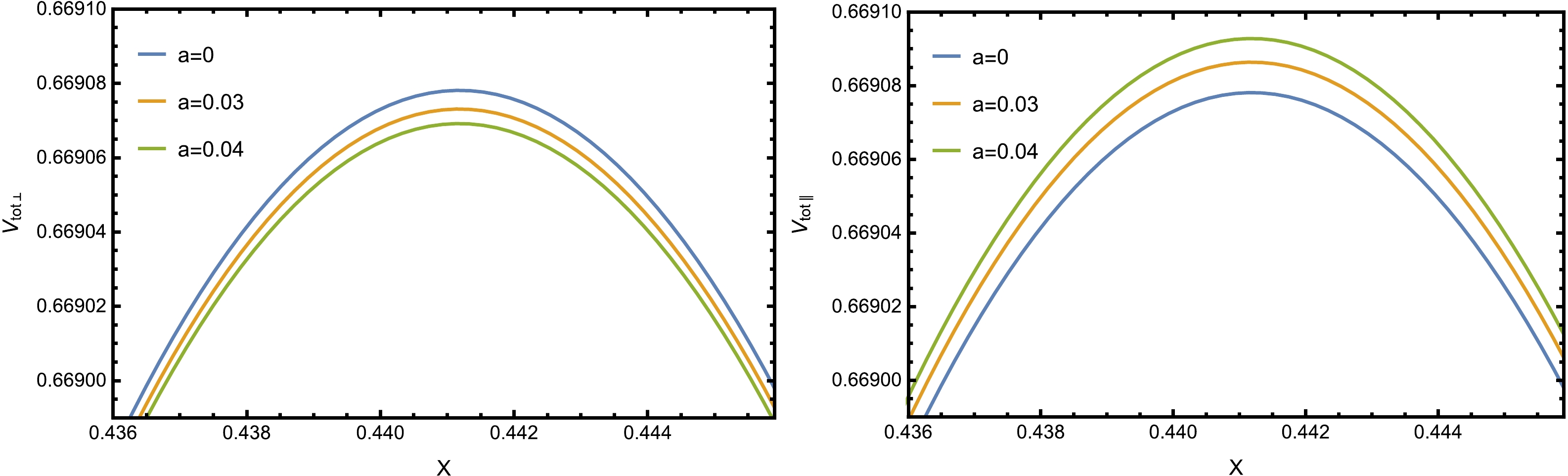
Figure 4. (color online) Total potential
$V_{\rm tot}$ as a function of the separation length x when$T=0.1 ~{\rm GeV}$ ,$\lambda_{\rm GB}=0.01$ , and$ \alpha = 0.6 $ . Left: The pair and the electric field are perpendicular to the anisotropy. Right: The pair and the electric field are parallel to the anisotropy.Moreover, to investigate the effect of anisotropy on the critical electric field, we plot
$ E_c $ as a function of the anisotropy parameter a when$T=0.1 ~{\rm GeV}$ and$\lambda_{\rm GB}=0.01$ in Fig. 5. We can see that$ E_{c} $ shows a slight decrease with an increase in a in the perpendicular case, which suggests that increasing the anisotropy strengthens the Schwinger effect. In contrast,$ E_{c} $ significantly rises with a in the parallel case, thus reducing the Schwinger effect. This result is consistent with the findings shown in Fig. 4.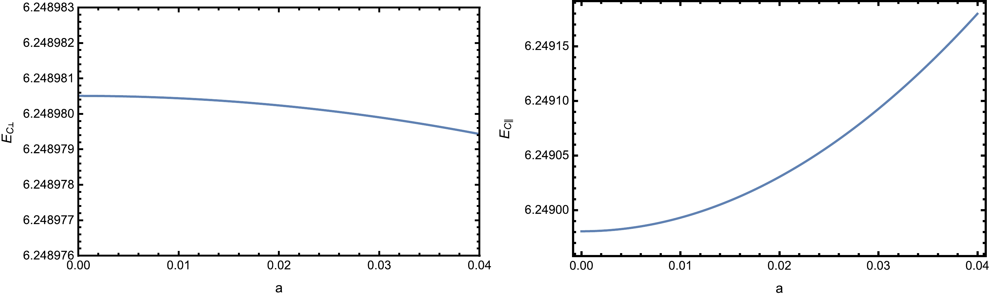
Figure 5. (color online)
$ E_c $ versus the anisotropy parameter a when$T=0.1 ~{\rm GeV}$ and$\lambda_{\rm GB}=0.01$ . Left: The the electric field is perpendicular to the anisotropy. Right: The electric field is parallel to the anisotropy. -
In Fig. 6, we plot the total potential
$V_{\rm tot}$ against x for$\alpha= 0.3,~ 0.6,~ 1.0$ , and$ 1.3 $ , when$T=0.1 ~{\rm GeV}$ ,$a=0.03$ GeV, and$\lambda_{\rm GB}=0.05$ . We can see that when$ \alpha < 1 $ , the potential barrier exists and$V_{\rm tot}$ decreases as the electric field becomes greater. When$ \alpha \ge 1 $ , the production of the particle pairs is simpler.
Figure 6. (color online) Total potential
$V_{\rm tot}$ as a function of the separation length x for different values of α when$T=0.1 ~{\rm GeV}$ ,$a=0.03 ~{\rm GeV}$ , and$\lambda_{\rm GB}=0.05$ . Left: The pair and the electric field are perpendicular to the anisotropy. Right: The pair and the electric field are parallel to the anisotropy.In order to determine how the Gauss-Bonnet coupling modifies the Schwinger effect, we plot the potential
$V_{\rm tot}$ versus x with$ \alpha = 0.3 $ for different values of$\lambda_{\rm GB}$ in Fig. 7. From the figure, we can see that in both cases, the height and width of$V_{\rm tot}$ decrease as$\lambda_{\rm GB}$ increases for a fixed α. Therefore, one might infer that the existence of the Gauss-Bonnet coupling reduces the potential barrier, thus enhancing the Schwinger effect, which is in agreement with the calculations of [19, 20].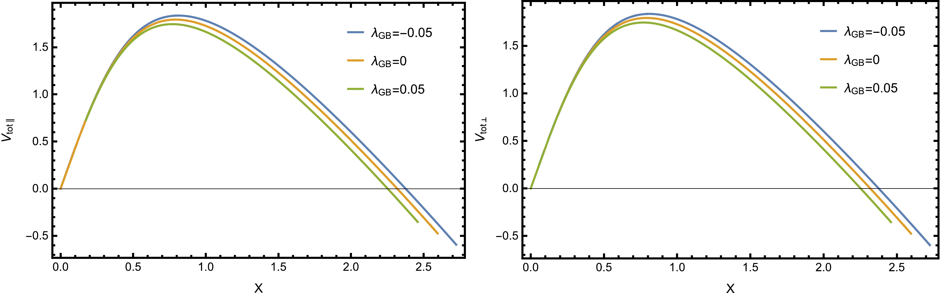
Figure 7. (color online) Total potential
$V_{\rm tot}$ as a function of the separation length x when$T=0.1 ~{\rm GeV}$ ,$a=0.03 ~{\rm GeV}$ , and$ \alpha = 0.3 $ . Left: The pair and the electric field are perpendicular to the anisotropy. Right: The pair and the electric field are parallel to the anisotropy.Further, to understand how the Gauss-Bonnet coupling influences the critical electric field, we plot
$ E_c $ against$\lambda_{\rm GB}$ in Fig. 8. It is found that$ E_c $ decreases when$\lambda_{\rm GB}$ increases; thus, the Schwinger effect is more likely to occur when the Gauss-Bonnet coupling exists, which is in line with the previous potential analysis.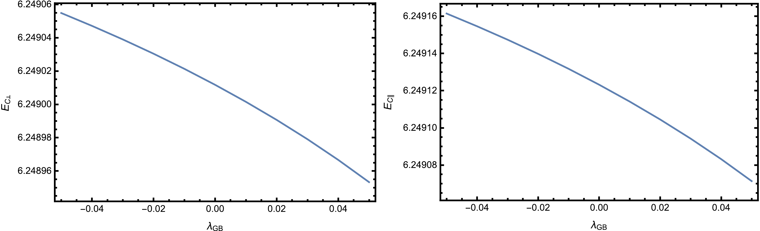
Figure 8. (color online)
$ E_c $ against the Gauss-Bonnet coupling parameter$\lambda_{\rm GB}$ when$T=0.1 ~{\rm GeV}$ and$a=0.03 ~{\rm GeV}$ . Left: The electric field is perpendicular to the anisotropy. Right: The electric field is parallel to the anisotropy. -
In this study, we investigated the effect of anisotropy and the Gauss-Bonnet coupling on the holographic Schwinger effect by considering a 5-dimensional AdS-axion-dilaton system with a Gauss-Bonnet term. By utilizing the AdS/CFT correspondence, we analyzed the total potential of the particle pair in an external electric field and calculated the critical value for the electric field via DBI action. The results indicate that the anisotropy and Gauss-Bonnet coupling can modify the total potential and the critical electric field in different ways, hence affecting the Schwinger effect.
When the particle pair and the electric field are perpendicular to the anisotropy, the potential barrier will be reduced due to the effect of the anisotropy, thus enhancing the Schwinger effect. Meanwhile, in the parallel case, the anisotropy tends to increase the potential barrier, thus weakening the Schwinger effect. The modification of quark tension by anisotropy, which increases in the parallel case and decreases in the perpendicular one, may be an interpretation of this result [38]. Regarding the Gauss-Bonnet coupling, in both the parallel and perpendicular cases, the potential barrier decreases as the Gauss-Bonnet coupling increases, thus favoring the Schwinger effect. Moreover, we note that the results of the potential analysis and the calculations of the critical electric field from the DBI action are in agreement.
Finally, it will be interesting to study the Schwinger effect in a spatially-dependent or time-dependent anisotropy background, which we will leave for further research.
-
We thank Zi-qiang Zhang, Xun Chen, and Viktor Jahnke for their fruitful discussions.
Holographic Schwinger effect in an anisotropic background with Gauss-Bonnet corrections
- Received Date: 2023-07-02
- Available Online: 2023-11-15
Abstract: Using the anti-de Sitter/conformal field theory (AdS/CFT) correspondence, we study the holographic Schwinger effect in an anisotropic background with the Gauss-Bonnet term. As the background geometry is anisotropic, we consider both cases of the test particle pair and the electric field perpendicular to and parallel to the anisotropic direction. It is shown that the Schwinger effect is enhanced in the perpendicular case when anisotropy rises. In the parallel case, this effect is reversed. Additionally, the potential barrier and the critical electric field in the parallel case are more significantly modified by anisotropy compared to the perpendicular case. We also find that the presence of the Gauss-Bonnet coupling tends to increase the Schwinger effect.


 DownLoad: