


 Abstract
 HTML
HTML Reference
 Related
 PDF
PDF


-
Deep inelastic scattering (DIS) is an important process in high energy physics as it can define and measure parton densities, which are instrumental to computing hard processes and testing quantum chromodynamics (QCD) [1]. According to the collinear factorization theorem, parton distribution functions (PDFs) are key in investigating the proton structure function and describing the cross sections in hard processes. In particular, scattering cross sections can be expressed in terms of parton densities, which are universal and process independent. An accurate determination of PDFs is therefore necessary to improve our understanding of QCD. PDFs are functions of the parton momentum fraction x and the virtuality of the photon
$ Q^2 $ . Generally, the parameterization of PDFs is set at the initial scale$ Q_0^2 $ , and the value at a higher$ Q^2 $ is obtained through DGLAP evolution [2−5]. Therefore, the DGLAP evolution equations are standard tools in the theoretical investigation of PDFs.The evolution equations for PDFs are expressed in terms of the splitting functions that can be expanded in powers of the running coupling
$ \alpha_s $ . By considering a higher order of$ \alpha_s $ , one can obtain a higher accuracy of PDFs. However, this does not mean that the accuracy can be improved without any restrictions. It is difficult to derive higher order splitting functions. However, higher order DGLAP evolution equations are numerically and analytically difficult to solve as they are complex integro-differential equations. In the literature, the DGLAP equations can be numerically solved by iterating the evolution over infinitesimal steps in x [6] using Mellin moments and their inversion [7] and by expanding parton distributions and splitting functions on Laguerre polynomials [8]. There are various easy-to-use programs to perform DGLAP evolution, e.g., QCDNUM [9], QCD-PEGASUS [10], and CANDIA [11]. However, obtaining numerical solutions with high accuracy is time-consuming. Furthermore, the numerical solution becomes worse at small-x [12, 13]. Therefore, analytical solutions are more convenient for analyzing the asymptotic behavior of PDFs. Currently, obtaining the exact analytic solutions of the DGLAP evolution equations in the entire range of x and$ Q^2 $ is difficult. However, they can be solved under certain conditions. For example, gluon distributions are obtained using the Mellin transform under the double logarithmic approximation (DLA) [14]. The spin-independent and spin-dependent structure functions are obtained using Taylor expansion [15, 16]. The leading order (LO) singlet DGLAP evolution equations are solved using the Laplace transform [17, 18]. These approximated solutions successfully describe the structure functions under certain conditions, improving our understanding of the asymptotic behavior of PDFs.The splitting function is the input for the DGLAP evolution equation. The power of
$ \alpha_s $ in the splitting functions is typically used to denote the order of the DGLAP evolution equation. In LO accuracy, the splitting functions$ P_{gq} $ and$ P_{gg} $ are singular at small-x. Thus, the gluon distribution runs faster than the quark distribution at small-x, that is, the gluons are dominant at small-x. Indeed, the analytical solution of DGLAP evolution for the gluon distribution in the DLA exhibits a faster increase at small-x. The increase in the gluon distribution will lead to an increase in the quark distribution and eventually an increase in the structure function [14]. Therefore, the analysis of the asymptotic behavior of PDFs is important for the description of the measured quantities, e.g., the structure functions. In this study, we investigate the gluon distribution in the small-x limit up to next-to-leading order (NLO). Using the Mellin transform, we obtain an approximate solution for the gluon distribution and find that our analytical solution is consistent with the gluon distribution behavior of CJ15 in the small-x and large$ Q^2 $ regions.The rest of the paper is organized as follows. In the next section, we present the gluon distribution from DGLAP evolution with the NLO splitting function and give a detailed derivation of the analytical solution in the small-x limit using the Mellin transform. In Sec. III, the fitting procedure is presented and the fit results are discussed. Then, we investigate the DGLAP evolution of the proton structure function in Sec. IV. The main results of our study are summarized in Sec. V.
-
Ignoring the quark contribution to the gluon rich distribution function at small-x, the coupled DGLAP equation is
$ \frac{\partial g(x,Q^2)}{\partial \ln\dfrac{Q^2}{\Lambda^2}}\Big|_{\mathrm{DGLAP}}=\int_{x}^{1}P_{\mathrm{gg}}(z)g\left(\frac xz,Q^2\right)\frac{\mathrm{d}z}{z}, $

(1) where
$ P_{gg} $ is the splitting function. If considering up to the NLO terms,$ P_{gg} $ can be expanded as powers of$ \alpha_s(Q^2) $ [19],$ \begin{array}{*{20}{l}} \begin{aligned} P_\mathrm{gg}(z)&=\frac{\alpha_s(Q^2)}{2\pi}P_\mathrm{gg}^0(z)+ \left(\frac{\alpha_s(Q^2)}{2\pi}\right)^2P_\mathrm{gg}^1(z). \end{aligned} \end{array} $

(2) Here, the LO splitting function is
$ \begin{aligned}[b] {P_\mathrm{gg}}^0(z)=\;&2N_c\left[\frac{1-z}z+\frac {z}{(1-z)_+}+z(1-z)\right]\\&+\left(\frac{11}2-\frac{2N_f}3\right)\delta(1-z), \end{aligned} $

(3) and the NLO splitting function is
$ \begin{aligned}[b]\\[-5pt] P_{gg}^{1}(z)=\;& \begin{aligned}C_FT_f\left[-16+8z+\frac{20z^2}{3}+\frac{4}{3z}-(6+10z)\ln z-2(1+z)\ln^2z\right]\end{aligned} +N_cT_f\left[2-2z+\frac{26}9\left(z^2-\frac1 z\right)-\frac43(1+z)\ln z-\frac{20}9p(z)\right] \\ &+N_c^2\left[\frac{27(1-z)}2+\frac{67}9\left(z^2-\frac1 z\right)-\left(\frac{25}3-\frac{11z}3+\frac{44z^2}3\right)\ln z\right.+4(1+z)\ln^2z+\left(\frac{67}9+\ln^2z-\frac{\pi^2}3\right)p(z) \\ &-\left.4\ln z\ln(1-z)p(z)+2p(-z)S_2(z)\right] . \end{aligned} $ 
(4) At small fraction momentum, the z-integral may receive extra enhancement from the small-z region [14]. Therefore, the splitting function can be approximated as
$ P_{gg}(z)|_{z\ll1}\approx 2N_c+\frac{\alpha_s(Q^2)}{2\pi}H, $

(5) where H is defined as
$ H = C_F T_f (\dfrac{4}{3})+N_c T_f (-\dfrac{46}{9}) $ .With the approximation in Eq. (5), the DGLAP equation can be rewritten as
$ \frac{\partial g(x,Q^2)}{\partial \ln\frac{Q^2}{\Lambda^2}}\Big|_{\mathrm{DGLAP}} = \frac{\alpha_s(Q^2)}{2\pi} \int_{x}^{1} \left( 2N_c + \frac{\alpha_s(Q^2)}{2\pi}H \right)g\left(\frac x z,Q^2\right)\frac{\mathrm{d}z}{z^2}. $

(6) To obtain the analytical solution for Eq. (6), we rewrite the DGLAP equation in moment space using the Mellin transform
$ Q^2\frac{\partial g_\omega(Q^2)}{\partial Q^2}=\frac{\alpha_s(Q^2)}{2\pi}\left(2N_c+\frac{\alpha_s(Q^2)}{2\pi}H\right)\frac1\omega g_\omega(Q^2) . $

(7) Here,
$ G_\omega(Q^2) $ is the gluon distribution in Mellin space,$ \begin{aligned}[b] g_\omega(Q^2)=\;&\exp\Bigg\{\int_{Q_0^2}^{Q^2}\frac{{\rm d}Q^{\prime2}}{Q^{\prime2}}\\& \times\Bigg[\frac{\alpha_s(Q^2)}{2\pi}\Bigg(2N_c+\frac{\alpha_s(Q^2)}{2\pi}H\Bigg) \Bigg] \frac{1}{\omega}\Bigg\}g_\omega(Q_0^2) ,\end{aligned} $

(8) where
$ g_\omega(Q_0^2) $ is the initial gluon distribution in Mellin space. The running coupling at LO and NLO respectively take the form$ \frac{\alpha_s^\mathrm{LO}}{2\pi}=\frac{2}{\beta_0t}, $

(9) $ \frac{\alpha_s^{\mathrm{NLO}}}{2\pi}=\frac{2}{\beta_0t}\left(1-\frac{\beta_1\mathrm{ln}t}{\beta_0^2t}\right), $

(10) where
$ \beta_0=\dfrac13(33-2N_f) $ ,$ \beta_1=102-\dfrac{38}3N_f $ , and$ t=\ln\dfrac{Q^2}{\Lambda^2} $ . Inverting the Mellin transform, we obtain$ \begin{aligned}[b] G(x,Q^2)=\;&\int_{a-{\rm i}\infty}^{a+{\rm i} \infty}\frac{{\rm d}\omega}{2\pi {\rm i}}\exp\Bigg\{\omega\ln\frac1x+\int_{Q_0^2}^{Q^2}\frac{{\rm d}Q^{\prime2}}{Q^{\prime2}}\\&\times \Bigg[\frac{\alpha_s(Q^2)}{2\pi}\Bigg(2N_c+\frac{\alpha_s(Q^2)}{2\pi}H\Bigg) \Bigg]\frac{1}{\omega}\Bigg\}g_\omega(Q_0^2), \end{aligned} $

(11) where
$ G(x,Q^2)=xg(x,Q^2) $ . Here, we define$ \rho(Q^2)=\int_{Q_0^2}^{Q^2}\frac{{\rm d}Q^{\prime2}}{Q^{\prime2}}\left[\frac{\alpha_s(Q^{\prime2})}{2\pi}\left(2N_c+\frac{\alpha_s(Q^{\prime2})}{2\pi}H\right) \right], $

(12) $ P(\omega)=\omega\ln\frac1x + \frac{\rho(Q^2)}{\omega}. $

(13) Note that the factor
$ 2N_c+\dfrac{\alpha_s(Q^{\prime2})}{2\pi}H $ reduces to$ 2N_c $ when one from NLO goes to LO. To analyze the asymptotic behavior of the gluon distribution in Eq. (11) in the small fraction momentum limit, the saddle points of the exponent$ P(\omega) $ must be found, which are defined by the condition$ P^{\prime}(\omega=\omega_{sp})=0 $ . For Eq. (13), the saddle points are$ \omega_{sp}=\pm \sqrt{\frac{\rho(Q^2)}{\ln(1/x)}}. $

(14) Applying Taylor expansion around the saddle point up to the second order, Eq. (13) becomes
$ P(\omega)\approx P(\omega_{sp})+\frac12P^{\prime\prime}(\omega_{sp})(\omega-\omega_{sp})^2 , $

(15) where the term
$ \omega-\omega_{sp} $ is zero at the saddle points. A new integration variable ω is defined by$\omega-\omega_{sp}\equiv {\rm i}w$ [14], and then Eq. (11) becomes$ G(x,Q^2)\approx {\rm e}^{P(\omega_{sp})}g_{\omega_{sp}}(Q_0^2)\int_{-\infty}^\infty\frac{{\rm d}w}{2\pi}{\rm e}^{-P^{\prime\prime}(\omega_{sp})w^2/2}. $

(16) The result of performing ω-integration is
$ \begin{aligned}[b] G(x,Q^2)\approx\;& \frac{g_{\omega_{sp}}(Q_0^2)}{\sqrt{4\pi}}(\rho)^{1/4}(\ln(1/x))^{-3/4} \\&\times \rm{exp}\left(2\sqrt{\rho\ln(1/x)} \right). \end{aligned} $

(17) For small-x and large
$ Q^2 $ , the gluon distribution may be rewritten as$ \begin{array}{*{20}{l}} G(x,Q^2)\sim \, \rm{exp}\left(2\sqrt{\rho\ln(1/x)}\right), \end{array} $

(18) where the solution of NLO or LO of the DGLAP equation depends on
$ \rho(Q^2) $ . For the LO case,$ \rho(Q^2) $ is expressed as$ \rho^{\mathrm{LO}}(Q^2)=\frac{4N_c}{\beta_0}\ln \frac{t}{t_0}, $

(19) where
$ t=\ln\dfrac{Q^2}{\Lambda^2} $ and$ t_0=\ln \dfrac{Q_0^2}{\Lambda^2} $ . For the NLO case, it is difficult to obtain an analytic expression for$ \rho(Q^2) $ directly. However, the relationship between$ \rho^{\mathrm{NLO}}(Q^2) $ and$ \rho^{\mathrm{LO}}(Q^2) $ can be expressed as$ \frac{\rho^{\mathrm{NLO}}(Q^2)}{\rho^{\mathrm{LO}}(Q^2)}=\mathrm{R}(Q^2). $

(20) From Ralston's calculations [20], a boundary condition (
$ K(Q^2) $ ) is provided, and the gluon distribution is written as$ \begin{aligned}[b] & G(x,Q^2)=K(Q^2)\times \rm{exp}\left(2\sqrt{\rho\ln(1/x)}\right), \\ & K\left(Q^2\right)=a\left[\exp \left(\xi-\xi_0\right)+ b\right]\times \exp \left[c\left(\xi-\xi_0\right)^{1 / 2}\right] , \end{aligned} $

(21) where
$\xi=\ln \ln (Q^2/\Lambda^2_{\rm QCD})$ and$\xi_0=\ln \ln (Q_0^2/\Lambda^2_{\rm QCD})$ . In addition, when the gluon emission kernel has a "ladder" structure, the gluon distribution can be considered as [21]$ \begin{array}{*{20}{l}} G(x,Q^2)\sim \, {I_0}\left(2\sqrt{\rho\ln(1/x)}\right), \end{array} $

(22) where
${I}_0$ is the modified Bessel function. Therefore, the gluon distribution in Eq. (21) is rewritten as$ \begin{array}{*{20}{l}} \begin{aligned} & G(x,Q^2)=K(Q^2)\times {I_0}\left(2\sqrt{\rho\ln(1/x)}\right). \end{aligned} \end{array} $

(23) In the next section, we use our analytical results to fit the gluon distribution data. To obtain reasonable results, we replace
${I_0}\left(2(\rho\ln(1/x))^{1/2}\right)$ with${I_0}\left(2(\rho\ln(1/x))^{d}\right)$ in Eq. (23) and$ \mathrm{exp}\left(2(\rho\ln(1/x))^{1/2}\right) $ with$ \mathrm{exp}\left(2(\rho\ln(1/x))^{d}\right) $ in Eq. (21), where d is a free parameter around 0.5. -
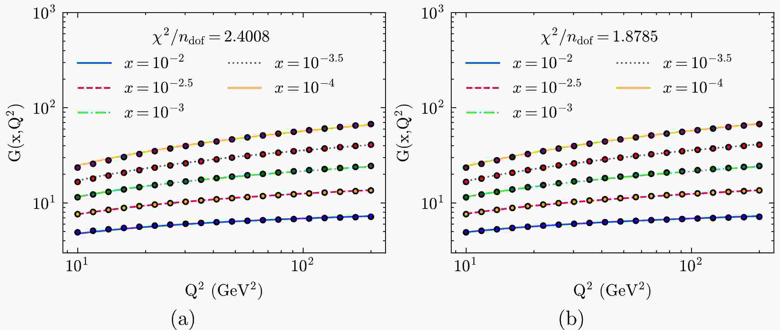
In this study, we use our analytical results to fit the CJ15 data [22, 23] in the
$10\,\;\mathrm{GeV^2} < Q^2 < 200\,\;\mathrm{GeV^2}$ and$ 10^{-4}<x<10^{-2} $ region. The results of the fits are presented in Table 1 , where S1 (S2) represents the fitting with Eq. (21) (Eq. (23)). Figure 1 shows the fitting results from CJ15LO data with Eqs. (21) and (23). The value of$ Q^2_0 $ at LO is set to be$ 1\,\mathrm{GeV^2} $ . As shown in Fig. 1(b), our solution in the S2 situation is in good agreement with the CJ15LO gluon distribution. We find that the value of d does not deviate much from 0.5.LO (S1) LO (S2) NLO (S1) NLO (S2) a $ 52.579\,\pm \,3.442 $ 

$ 185.446\,\pm \,3.254 $ 

20.658 $ \pm \,1.898 $ 

110.078 $ \pm \,8.871 $ 

b $ -1.205\,\pm \,0.014 $ 

$ -1.174\,\pm \,0.004 $ 

$-0.977 \pm \,0.018 $ 

$ -1.023\pm \,0.013 $ 

c $ -7.639\,\pm \,0.058 $ 

$ -7.463\,\pm \,0.016 $ 

$ -7.305\pm \,0.092 $ 

$-7.234 \pm \,0.083 $ 

d $ 0.505\,\pm \,2\times10^{-4} $ 

$ 0.522\,\pm \,2\times10^{-4} $ 

$ 0.431 \pm \,10^{-3} $ 

$0.454 \pm \,10^{-3} $ 

$ \chi^2/dof $ 

$ 2.4008 $ 

$ 1.8785 $ 

3.3476 1.2921 Table 1. Parameters and
$ \chi^2/dof $ from the fit to the CJ15LO and CJ15NLO data at LO and NLO, respectively. S1 represents the fitting with Eq. (21) and S2 denotes the fitting with Eq. (23).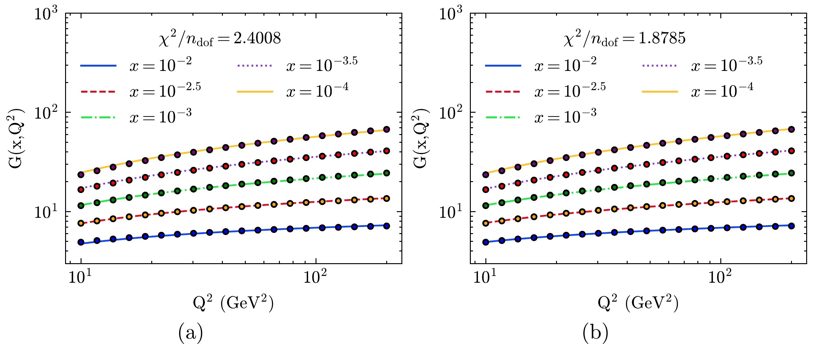
Figure 1. (color online) Fitting to the CJ15LO gluon distribution with four parameters in the
$10\;\,\mathrm{GeV^2} < Q^2 <200\,\;\mathrm{GeV^2}$ and$ 10^{-4}<x<10^{-2} $ region with Eqs. (21) (left panel) and (23) (right panel).When NLO corrections are considered,
$ \rho^{\mathrm{NLO}} $ is used. As described in the previous section, it is difficult to obtain an analytic form of$ \rho^{\mathrm{NLO}} $ . However, it can be described using Eqs. (19) and (20) as$ \rho^{\mathrm{NLO}}=\left(\frac{4N_c}{\beta_0}\ln \frac{t}{t_0}\right)R(t). $

(24) Therefore, it is helpful to express
$ \rho^{\mathrm{NLO}} $ with$ \rho^{\mathrm{LO}} $ and$ R(t) $ . The numerical results of$ R(t) $ show that$ R(t) $ varies monotonically with t. Meanwhile,$ \rho^{\mathrm{NLO}}\approx \rho^{\mathrm{LO}} $ when$ t\rightarrow \infty $ . Based on these two facts, we attempt to construct a function to describe the ratio between$ \rho^{\mathrm{NLO}} $ and$ \rho^{\mathrm{LO}} $ . We find that$ R(t) $ can be written as${\tilde{a}t^{\tilde{d}}}/({\tilde{b}+\tilde{c}t^{\tilde{e}}})$ with the free parameters$ \tilde{a} $ ,$ \tilde{b} $ ,$ \tilde{c} $ ,$ \tilde{d} $ , and$\tilde{e}$ . When$Q^2_0=2.5\,\;\mathrm{GeV}^2$ ,$\tilde{a}= $ $13.115,\,\tilde{b}=14.638, \,\tilde{c}=19.065,\; \tilde{d}=0.665, \;\,\tilde{e}=0.616$ . Figure 2 shows our model agrees with the numerical results.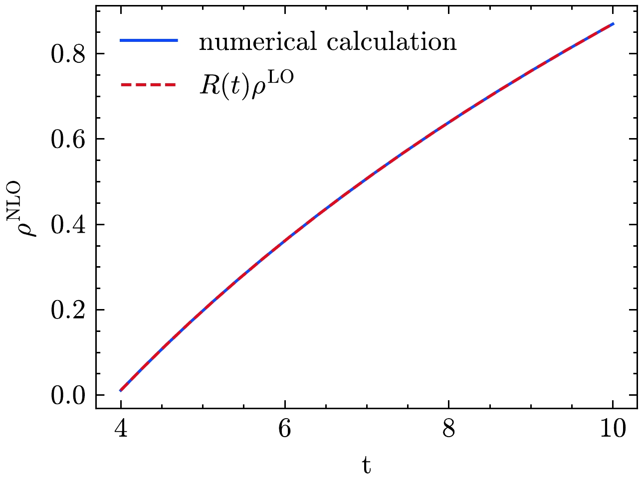
Figure 2. (color online) Results of
$ \rho^{\mathrm{NLO}} $ . The blue solid line represents the results calculated using the numerical method, and the red dashed line represents the results calculated using$ R(t)\rho^{\mathrm{LO}} $ .With the analytical expression of
$ R(t) $ , we can obtain the fitting results with NLO corrections. Figure 3 shows the fitting results from CJ15LO data with Eqs. (21) and (23). The values of the fitting parameters are also listed in Table 1. In the larger$ Q^2 $ region, our models are in good agreement with CJ15NLO. Compared with the fitting result with Eq. (21), the gluon distribution from Eq. (23) is more favored by the data. The value of d is less than 0.5 but not far off. Overall, our model is able to reproduce the gluon behavior at CJ15NLO in certain regions.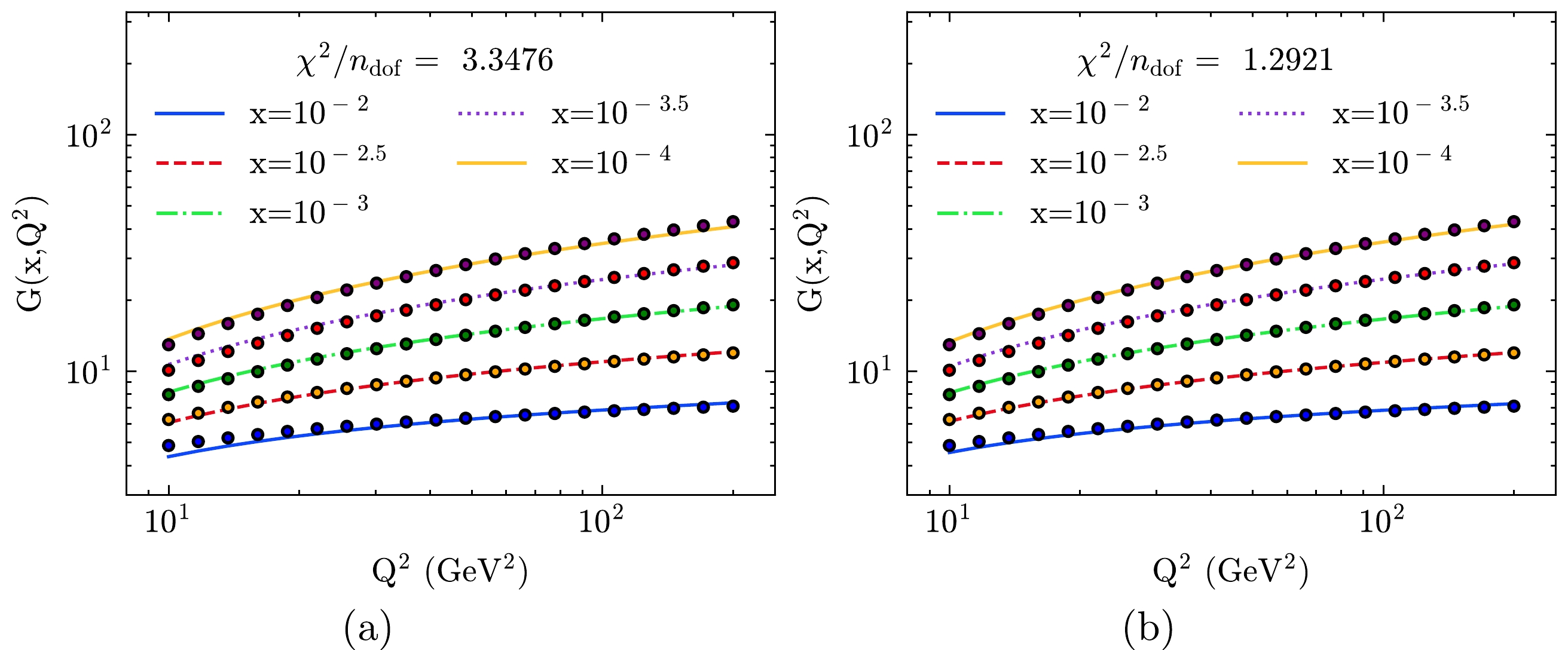
Figure 3. (color online) Fitting to the CJ15NLO gluon distribution with four parameters in the
$10\,\;\mathrm{GeV^2} < Q^2 < 200\,\;\mathrm{GeV^2}$ and$ 10^{-4}<x<10^{-2} $ region with Eqs. (21) (left panel) and (23) (right panel). -
In the small-x region, when only the gluon contribution is considered, the DGLAP evolution equation for the proton structure function
$ F_2 $ can be written as [24−26]$ \begin{array}{*{20}{l}} \begin{aligned} \frac{\partial F_{2}(x,Q^{2})}{\partial\ln Q^{2}} = \frac{20}{9}\frac{\alpha_{s}}{2\pi}\int_{x}^{1}{\rm dz}P_{qg}(z)G\left(\frac{x}{z},Q^{2}\right). \end{aligned} \end{array} $

(25) Here, the splitting function
$ P_{qg}(z) $ is defined as$ P_{qg}(z)=P^{\mathrm{LO}}_{qg}(z)+\frac{\alpha_s}{2\pi}P^{\mathrm{NLO}}_{qg}(z), $

(26) for which splitting functions can be found in [25]. When
$ P^{\mathrm{LO}}_{qg}(z) $ is contained only by expanding the gluon distribution around$ z=\dfrac{1}{2} $ , Prytz's approach for the$ F_2 $ evolution function is written as [27]$ \frac{\partial F_{2}(x,Q^{2})}{\partial\ln Q^{2}}|_{\mathrm{LO}} \approx \frac{20}{27}\frac{\alpha_s}{2\pi}G(2x). $

(27) Alternatively, expanding the gluon distribution around
$ z=0 $ , Bora's approach for the$F_2$ evolution function is given as [28, 29]$ \frac{\partial F_{2}(x,Q^{2})}{\partial\ln Q^{2}}\Big|_{\mathrm{LO}} \approx \frac{20}{27}\frac{\alpha_s}{2\pi}G(\frac{3}{2}x). $

(28) Once the NLO corrections are considered,
$ \dfrac{\partial F_{2}(x,Q^{2})}{\partial\ln Q^{2}} $ is given as$ \begin{aligned}[b] \frac{\partial F_{2}(x,Q^{2})}{\partial\ln Q^{2}} \approx\;& \frac{\partial F_{2}(x,Q^{2})}{\partial\ln Q^{2}}|_{\mathrm{LO}}+ \frac{20}{9}\left(\frac{\alpha_{s}}{2\pi}\right)^2\\&\times\int_{x}^{1}{\rm d}zP^{\mathrm{NLO}}_{qg}(z)G\left(\frac{x}{z},Q^{2}\right). \end{aligned} $

(29) A simple form of
$ P^{\mathrm{NLO}}_{qg} $ may be considered in the small-x limit [26, 30],$ P^{\mathrm{NLO}}_{qg}\rightarrow \frac{\alpha_s}{2\pi}\frac{60}{9z}. $

(30) Therefore,
$ \dfrac{\partial F_{2}(x,Q^{2})}{\partial\ln Q^{2}} $ is rewritten as$ \begin{aligned}[b] \frac{\partial F_{2}(x,Q^{2})}{\partial\ln Q^{2}} \approx\;& \frac{\partial F_{2}(x,Q^{2})}{\partial\ln Q^{2}}\Big|_{\mathrm{LO}}\\&+ \frac{1200}{81} \left(\frac{\alpha_{s}}{2\pi}\right)^2 \int_{x}^{1}{\rm d}z \frac{1}{z}G\left(\frac{x}{z},Q^{2}\right). \end{aligned} $

(31) Here, we expand the second term on the right-hand side of Eq. (31) around an arbitrary point α in the same way [29].
$\int_{x}^{1}{\rm d}z \dfrac{1}{z}G\left(\dfrac{x}{z},Q^{2}\right)$ can be written as$ \begin{aligned}[b] \int_{x}^{1}{\rm d}z \,\frac{1}{z}\, G\left(\frac{x}{z},Q^{2}\right) &=\frac{1}{x}\int_{x}^{1}{\rm d}z \tilde{G}\left(\frac{x}{z},Q^{2}\right)\\&=\frac{1}{x}\int^{1-x}_{0}{\rm d}\tilde{z} \tilde{G}\left(\frac{x}{1-\tilde{z}},Q^{2}\right), \end{aligned} $

(32) where
$ \tilde{G}(x,Q^2)=xG(x,Q^2) $ . Then, expanding$ \tilde{G} $ at$ z=\alpha $ up to the first order, we get$ \begin{aligned}[b] \frac{1}{x}\int^{1-x}_{0}{\rm d}\tilde{z} \tilde{G}\left(\frac{x}{1-\tilde{z}},Q^{2}\right)\approx\;& \frac{1}{x}\int^{1-x}_{0}{\rm d}\tilde{z} \Bigg(\tilde{G}\left(\frac{x}{1-\alpha},Q^{2}\right)\\&+\frac{x(z-\alpha)}{(\alpha-1)^2}\tilde{G}\left(\frac{x}{1-\alpha},Q^{2}\right)\Bigg). \end{aligned}$

(33) In the small-x limit, Eq. (33) is written as
$ \begin{aligned}[b] \frac{1}{x}\int^{1-x}_{0}{\rm d}\tilde{z} \tilde{G}\left(\frac{x}{1-\tilde{z}},Q^{2}\right)\approx \frac{\left(1-x\right)}{x} \tilde{G}\left(\frac{{3}/{2}-2\alpha}{(1-\alpha)^2}x\right) \end{aligned} $

$ \begin{aligned}[b] \quad\quad =\left(1-x\right) \frac{{3}/{2}-2\alpha}{(1-\alpha)^2}G\left(\frac{{3}/{2}-2\alpha}{(1-\alpha)^2}x\right). \end{aligned} $

(34) Therefore, from Eq. (31), we have
$ \begin{aligned}[b] \frac{\partial F_{2}(x,Q^{2})}{\partial\ln Q^{2}} \approx\;& \frac{20}{27}\frac{\alpha_s}{2\pi}G(2x)+\frac{1200}{81} \left(\frac{\alpha_{s}}{2\pi}\right)^2 \\&\times\left(1-x\right) \frac{{3}/{2}-2\alpha}{(1-\alpha)^2}G\left(\frac{{3}/{2}-2\alpha}{(1-\alpha)^2}x\right). \end{aligned} $

(35) As shown in Fig. 4, the calculations of
$ \dfrac{\partial F_{2}(x,Q^{2})}{\partial\ln Q^{2}} $ are presented at LO and NLO. The black and blue solid lines represent the calculations using Bora's and Prytz's approaches at LO, respectively. The red dashed line represents the calculation of the differential structure function using CJ15NLO data [22] directly with Eq. (29), where no approximation is made to the NLO splitting function. The green dotted line represents our approximated solution for which Eq. (35) with$ \alpha=0.0 $ is used. For LO results, Fig. 4 shows that Prytz's and Bora's approaches are valid. When NLO corrections are contained, our result with the approximated solution is higher than the calculation of the differential structure function using CJ15NLO data directly with Eq. (29). When x decreases, the gap between these two calculations narrows, which is consistent with the fact that our model is valid in the small-x region.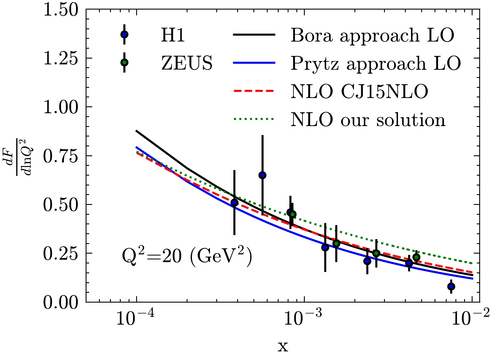
Figure 4. (color online) Differential structure function. Experimental data from H1 [31] and ZEUS [32]. The black and blue solid lines represent the calculation of the differential structure function using Bora's and Prytz's approaches at LO, respectively. The red dashed line represents the calculation of the differential structure function using CJ15NLO data [23] directly with Eq. (29). The green dotted line represents our approximated solution used with Eq. (35)
-
In this study, we use LO and NLO approximated solutions from the DGLAP equation to fit the gluon distributions of CJ15LO and CJ15NLO, respectively. The fitting results reveal that the LO and NLO approximated solutions are satisfactory in the small-x and large
$ Q^2 $ regions. Compared with the fitting result with Eq. (21), the gluon distribution from Eq. (23), in which the "ladder" structure of gluon emission is considered, is better. Then,$ \dfrac{\partial F_{2}(x,Q^{2})}{\partial\ln Q^{2}} $ is calculated with the LO and NLO approximated solutions at$ Q^2=20\,\mathrm{GeV^2} $ . Moreover,$ \dfrac{\partial F_{2}(x,Q^{2})}{\partial\ln Q^{2}} $ is given using Eq. (31) directly with the CJ15NLO gluon distribution. Our result from the approximated expression Eq. (35) is higher than the calculation from the CJ15NLO gluon distribution at larger x. This suggests that the approximation at large x is not valid. However, our approximated results have a similar tendency to CJ15 at small-x, which indicates that the approximation is valid for describing the asymptotic behavior at small-x.
Analysis of the gluon distribution with next-to-leading order splitting function at small-x
- Received Date: 2024-01-29
- Available Online: 2024-06-15
Abstract: An approximated solution for the gluon distribution from DGLAP evolution equations with the NLO splitting function in the small-x limit is presented. We first obtain simplified forms of the LO and NLO splitting functions in the small-x limit. With these approximated splitting functions, we obtain the analytical gluon distribution using the Mellin transform. The free parameters in the boundary conditions are obtained by fitting the CJ15 gluon distribution data. We find that the asymptotic behavior of the gluon distribution is consistent with the CJ15 data; however, the NLO results considering the "ladder" structure of gluon emission are slightly better than the LO results. These results indicate that the corrections from NLO have a significant influence on the behavior of the gluon distribution in the small-x region. In addition, we investigate the DGLAP evolution of the proton structure function using the analytical solution of the gluon distribution. The differential structure function reveals that our results have a similar tendency to the CJ15 data at small-x.


 DownLoad: