ρ-meson longitudinal leading-twist distribution amplitude revisited and the D→ρ semileptonic decay

I. INTRODUCTION

• I. INTRODUCTION
• II. THEORETICAL FRAMEWORK
• III. NUMERICAL ANALYSIS
• IV. SUMMARY
• ACKNOWLEDGMENTS

The ρ-meson leading-twist longitudinal distribution amplitude (DA) is a key input parameter when investigating related exclusive processes including the ρ meson. Charmed semileptonic decay processes can provide a clear platform for researching the ρ-meson DA. In charmed factories, the BESIII collaboration reported new results for the semileptonic decay $D^0\to \rho^-\mu^+\nu_\mu$ in 2021 [1]. In 2019, the BESIII collaboration provided improved measurements of $D\to\rho e^+\nu_e$ [2]. The CLEO collaboration provided measurements of the form factors in the decays $D^{0/+}\to \rho^{-/0}e^+\nu_e$ in 2013 [3], and their previous measurements can be found in [4, 5]. It is known that transition form factors (TFFs) are key components of semileptonic $D \to \rho \ell^+ \nu_\ell$ decays in the standard model. Therefore, accurate TFFs are very important for theoretical groups and experimental collaborations. Theoretically, the $D\to\rho$ TFFs can be treated using different approaches, such as the 3-point sum rule (3PSR) [6], heavy quark effective field theory (HQEFT) [7, 8], relativistic harmonic oscillator potential model (RHOPM) [9], quark model (QM) [10, 11], light-front quark model (LFQM) [12, 13], light-cone sum rule (LCSR) [14−16], covariant confined quark model (CCQM) [17], heavy meson and chiral symmetry theory (HMχT) [18], and lattice QCD (LQCD) [19, 20]. The LCSR approach is based on operator production expansion near the light-cone, and all the non-perturbative dynamics are parameterized into light-cone DAs (LCDAs), which is suitable for calculating the heavy to light transition. In this study, we take the LCSR approach to calculate the $D\to\rho$ TFFs with a left-handed current ¹. Thus, the key task is obtaining an accurate ρ-meson longitudinal twist-2 DA.

Theoretically, the ρ-meson longitudinal leading-twist DA can be studied using various methods, such as QCD sum rules (SRs) [21−26], LQCD [27−30], the AdS/QCD holographic method [31−34], extraction from experimental data [35−38], the light-front quark model (LFQM) [39, 40], Dyson-Schwinger equations (DSEs) [41], large momentum effective theory (LMET) [42], instanton vacuum [43, 44], and other models [45, 46]. The QCDSR in the framework of background field theory (BFT) is an effective approach in calculating light and heavy meson DAs [47]. In early 2016, we preliminarily studied the ρ-meson longitudinal leading-twist DA [48], in which the first two order nonzero ξ-moments and Gegenbauer moments were obtained, and the behavior of $\phi_{2;\rho}^\|(x,\mu)$ described by the light-cone harmonic oscillator (LCHO) model was determined [49].

In 2021, we proposed a new research scheme for the QCDSR study on pionic leading-twist DAs, in which a new SR formula for ξ-moments was proposed after considering that the SR for the zeroth ξ-moment cannot be normalized in the entire Borel region [50]. It enabled us to calculate more higher-order ξ-moments. Furthermore, the behavior of the pion DA $\phi_{2;\pi}(x,\mu)$ could be determined by fitting sufficient ξ-moments with the least squares method. Subsequently, this scheme was used to study pseudoscalar $\eta^{(\prime)}$-meson and kaon leading-twist DAs [51, 52] and D-meson twist-2,3 DAs [53], axial vector $a_1(1260)$-meson twist-2 longitudinal DAs [54], and scalar $a_0(980)$ and $K_0^\ast(1430)$-meson leading-twist DAs [55, 56]. Inspired by this, we restudy the ρ-meson leading-twist longitudinal DA $\phi_{2;\rho}^\|(x,\mu)$ by adopting the research scheme proposed in Ref. [50].

The remainder of this paper are organized as follows. In Sec. II, we present the calculations for the ξ-moments of the ρ-meson leading-twist DA, the $D\to \rho$ TFFs, and the semileptonic decays $D\to\rho\ell^+\nu_\ell$. In Sec. III, we present the numerical results and discussions on the ξ-moments, $D\to \rho$ TFFs, and $D\to \rho\ell^+\nu_\ell$ decay widths and branching ratios. Section IV is contains a summary.

II. THEORETICAL FRAMEWORK

• I. INTRODUCTION
• II. THEORETICAL FRAMEWORK
• III. NUMERICAL ANALYSIS
• IV. SUMMARY
• ACKNOWLEDGMENTS

To derive the sum rules of ρ-meson leading-twist longitudinal DA ξ-moments, we adopt the following correlation function (also known as the correlator):

where the current $J_n(x) = \bar{d} {\not {z}} ({\rm i}z\cdot {\mathop D\limits^ \leftrightarrow})^n u(x)$ with $z^2 = 0$. After taking the standard QCDSR calculation procedure within the framework of BFT [50], we obtain an expression for $\langle\xi^n\rangle_{2;\rho}^\| \times \langle\xi^0\rangle_{2;\rho}^\|$,

where $m_\rho$ and $f_\rho$ are the ρ-meson mass and decay constant, respectively, $s_\rho$ is the continuum threshold, $m_u$ and $m_d$ are the current quark masses of the u and d quarks, respectively, M is the Borel parameter, $\langle\bar{q}q\rangle$ with $q = u (d)$ is the double-quark condensate, $\langle\alpha_sG^2\rangle$ is the double-gluon condensate, $\langle g_s\bar{q}\sigma TGq\rangle$ is the quark-gluon mix condensate, $\langle g_s^3fG^3\rangle$ is the triple-gluon condensate, and $\langle g_s\bar{q}q \rangle^2$ and $\langle g_s^2\bar{q}q \rangle^2$ are the four-quark condensates, respectively. In addition, $\kappa = \langle\bar{s}s\rangle / \langle\bar{q}q\rangle$ with the double s quark condensate $\langle\bar{s}s\rangle$. By taking $n = 0$ for Eq. (2), the SR of the zeroth-order ξ-moment $\langle\xi^0\rangle_{2;\rho}^\|$ can be obtained as

Eq. (3) indicates that the zeroth-order ξ-moment $\langle\xi^0\rangle_{2;\rho}^{\|}$ in Eq. (2) cannot be normalized in the entire Borel parameter region. The main reason for this is because the contributions from vacuum condensates larger than dimension-six are truncated normally. As discussed in Ref. [50], a more accurate and reasonable SR for the nth-order ξ-moment $\langle\xi^n\rangle_{2;\rho}^\|$ should be

However, to describe the behavior of the ρ-meson leading-twist longitudinal DA, we take the following DSE model for $\phi_{2;\rho}^\parallel(x,\mu)$ [57, 58]:

where $\alpha_- = \alpha - 1/2$, and $\mathcal{N} = 4^\alpha \Gamma(\alpha + 1) / [\sqrt{\pi} \Gamma(\alpha + 1/2)]$ is the normalization constant. In this notation, the Gegenbauer polynomial series is considered the most accurate form for describing the meson DA. Unfortunately, one cannot obtain all Gegenbauer moments in principle. Therefore, a truncated form of the Gegenbauer polynomial series (TF model) is typically used to approximately describe the behavior of the meson DA in the literature. However, the TF model is not an ideal model for describing the behavior of meson DAs, because it truncates at the lowest Gegenbauer coefficient. In fact, the DSE model is still a truncated form of the Gegenbauer polynomial series. The difference between these two models is that the DSE model is based on the ${C_n^\alpha}$-basis, whereas the TF model is based on the ${C_n^{3/2}}$-basis. In addition, the factor $[x(1-x)]^{\alpha_-}$ in the DSE model can adjust and compensate for the impact caused by truncation to a certain extent. Another advantage of the DSE model is that, as mentioned in Ref. [58], it can reduce the introduced spurious oscillations.

Next, to obtain the $D\to\rho$ TFFs, we can take the following correlation function:

where $j_D^{L} (x)= {\rm i} \bar q_2(x)(1 - \gamma_5)c(x)$ is the left-handed current. As we know, there are fifteen DAs for a vector meson up to twist-4 accuracy, and the left-handed chiral current can reduce the uncertainties from chiral-odd vector meson DAs with $\delta^{0,2}$-order and leave the chiral-even with a $\delta^{1,3}$-order meson. The relationships are listed in Table 1. In this table, except $j_D^{L} (x)$, the current $j_D^{R} (x)$ respects the right-handed current with the expression $j_D^{R} (x)= {\rm i} \bar q_2(x) \times (1 + \gamma_5)c(x)$, as researched in our previous study [15]. The parameter $\delta \simeq m_\rho/m_c\sim 52\ $% [59, 60]. Meanwhile, the chiral current approach has been considered in other studies [61−66], which improves the predictions of the LCSR approach.

Table 1

Table 1.  ρ-meson DAs with different twist-structures up to $\delta^3$, where $\delta \simeq m_\rho/m_c$.

		twist-2	twist-3	twist-4
	$\delta^0$	$\phi_{2;\rho}^\bot$
$j_D^{L} (x)$	$\delta^2$		$\phi_{3;\rho}^\|, \psi_{3;\rho}^\|, \Phi_{3;\rho}^\bot$	$\phi_{4;\rho}^\bot,\psi_{4;\rho}^\bot,\Psi_{4;\rho}^\bot, \widetilde{\Psi} _{4;\rho}^\bot$
	$\delta^1$	$\phi_{2;\rho}^\|$	$\phi_{3;\rho}^\bot, \psi_{3;\rho}^\bot, \Phi_{3;\rho}^\|,\tilde\Phi_{3;\rho }^\bot$
$j_D^{R} (x)$	$\delta^3$			$\phi_{4;\rho}^\|,\psi_{4;\rho}^\|$

DownLoad: CSV

Show Table

Based on the procedures of the LCSR approach, we obtain the expressions of the $D\to \rho$ TFFs $A_{1,2}(q^2)$ and $V(q^2)$ LCSRs with the left-handed current in the correlator. The analytic formulas are similar to the $B\to\rho$ TFFs of our previous study [45], which replace the input parameter of the B-meson with a D-meson, such as $m_B\to m_D$, $f_B \to f_D$, $m_b \to m_c$. The detailed expressions can be written as follows:

where $s(\varrho)=[m_b^2-\bar \varrho(q^2-\varrho m_\rho^2)]/\varrho$ with $\bar \varrho = 1 - \varrho$ ($\varrho$ represents u or X), and $X=a_1 + v a_3$. $f_\rho^\|$ represents the ρ-meson decay constant, and $c(u,s_0)=u s_0 - m_b^2 + \bar u q^2 - u \bar u m_\rho^2$. $\Theta(c(\varrho,s_0))$ is the usual step function, and the definitions for $\widetilde\Theta (c(u,s_0))$, $\widetilde{\widetilde\Theta}(c(u,s_0))$, and $\widetilde{\widetilde{\widetilde\Theta}}(c(u,s_0))$ can be found in our previous study [45]. The combined ρ-meson DA $A_\rho^\| (x), B_\rho^\| (x)$, and $C_\rho^\| (x)$ have the expressions

which originate from the definition of the chiral-even two-particle DAs [60]. From Eqs. (7), (8), and (9), we can see that only $\delta^{1,3}$-order DAs have contributions to TFFs with a left-chiral correlation function. Conversely, $\delta^{0,2}$-order DAs do not have contributions, which also indicates that transverse twist-2 DAs have no contribution to $A_{1,2}(q^2)$ and $V(q^2)$. Furthermore, the twist-3 DAs $\psi_{3;\rho}^\bot(x,\mu)$, $\phi_{3;\rho}^\bot(x,\mu)$ , and $A_\rho^\| (x,\mu)$ can be related to $\phi_{2;\rho}^\|$ directly using the Wandzura-Wilczek approximation [67, 68],

Moreover, there have two ratio $r_V = {V(0)}/{A_1(0)}$ and $r_2={A_2(0)}/{A_1(0)}$ based on the TFFs $A_{1,2}(q^2)$ and $V(q^2)$, which have less uncertainties between the different approaches.

Next, we turn to the physical observables for the semileptonic decay $D\to\rho \ell^+\nu_\ell$. Therefore, we introduce the longitudinal and transverse helicity decay widths, which are composed in terms of three helicity form factors $H_{0,\pm} (q^2)$

where the constant $C_k = 1$ for $D^0\to\rho^-\ell^+\nu_\ell$ and $C_k = 1/\sqrt{2}$ for $D^+\to\rho^0\ell^+\nu_\ell$. Other parameters and expressions have the following definitions: $G_F=1.166\times10^{-5}\; {\rm GeV}^{-2}$ is the Fermi constant, $\lambda(q^2) = (m_D^2 + m_\rho^2 - q^2)^2-4 m_D^2 m_\rho^2$ is the phase-space factor, and $q^2_{\rm max} = (m_D-m_\rho)^2$ is the small recoil point of the $D\to\rho$ transition. The three helicity form factors $H_{\pm}(q^2)$ and $H_0(q^2)$ are mainly separated by the transition amplitude with a definite spin-parity quantum number, which can be found in our previous study [15]. Meanwhile, the longitudinal and transverse helicity amplitudes are expressed as $\Gamma^{\rm T} = \Gamma^+ + \Gamma^-$, $\Gamma^{\rm L}=\Gamma^0$ , and $\Gamma=\Gamma^{\rm L} + \Gamma^{\rm T}$. The helicity form factors $H_{0,\pm}(q^2)$ can be calculated by relating them to the Lorentz orthogonal form factors $A_{1,2}(q^2)$ and $V(q^2)$ via the following definition:

and

III. NUMERICAL ANALYSIS

• I. INTRODUCTION
• II. THEORETICAL FRAMEWORK
• III. NUMERICAL ANALYSIS
• IV. SUMMARY
• ACKNOWLEDGMENTS

To perform the numerical calculation, we take $f_\rho = 210 \pm 4\; {\rm MeV}$ [40, 69], $m_\rho = 775.26 \pm 0.23\; {\rm MeV}$, the current quark masses $m_u = 2.16^{+0.49}_{-0.26}\; {\rm MeV}$ and $m_d = 4.67^{+0.48}_{-0.17}\; {\rm MeV}$ [70], the vacuum condensates $\langle\bar{q}q\rangle = (-2.417^{+0.227}_{-0.114}) \times 10^{-2}\; {\rm GeV}^2$, $\langle g_s\bar{q}\sigma TGq\rangle = (-1.934^{+0.188}_{-0.103}) \times 10^{-2} {\rm GeV}^5$, $\langle g_s\bar{q}q\rangle^2 = (2.082^{+0.734}_{-0.697}) \times 10^{-3}\; {\rm GeV}^6$, $\langle g_s^2\bar{q}q\rangle^2 = (7.420^{+2.614}_{-2.483}) \times 10^{-3}\; {\rm GeV}^6$, $\langle\alpha_s G^2\rangle = 0.038 \pm 0.11\; {\rm GeV}^4$, and $\langle g_s^3fG\rangle \simeq 0.045\; {\rm GeV}^6$, and $\kappa = 0.74 \pm 0.03$ [50, 71, 72]. Among these, the current quark masses and vacuum condensates except the gluon condensates are scale dependent and have above values at $\mu = 2\; {\rm GeV}$. For the scale evolution of these inputs, refer to Ref. [50]. For the detailed calculation in this study, we take the scale $\mu = M$ as usual. By requiring that there be a reasonable Borel window to normalize $\langle\xi^0\rangle_{2;\rho}^\parallel$ with Eq. (3), we obtain the continuum threshold as $s_\rho \simeq 2.1\; {\rm GeV}^2$.

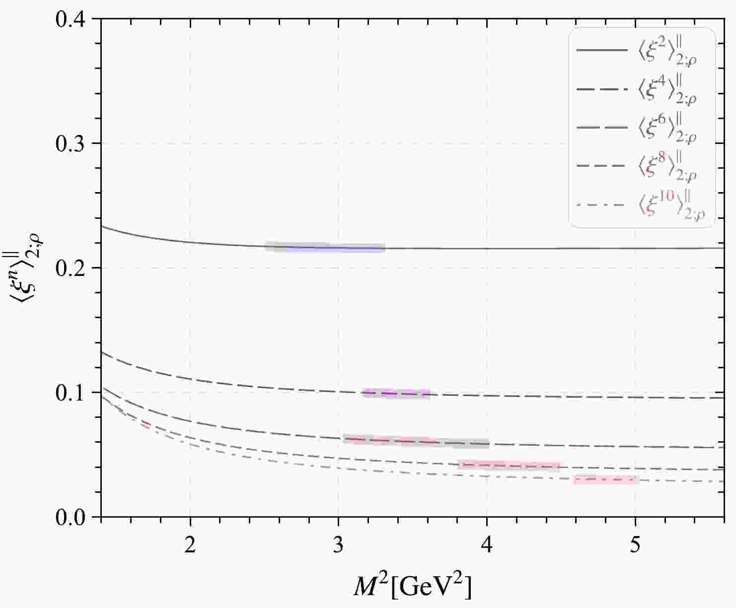
Now, we can obtain the ξ-moment versus the Borel parameter. Furthermore, we can determine the Borel window and then the value of the nth ξ-moment $\langle\xi^n\rangle_{2;\rho}^\parallel$ based on the well-known criteria that the contributions of the continuum state and dimension-six condensate are as small as possible and the value of $\langle\xi^n\rangle_{2;\rho}^\parallel$ is stable in the Borel window. Specifically, the continuum contribution is not more than $30$% for all of the nth-order, and the dimension-six contribution of $\langle\xi^n\rangle_{2;\rho}^\parallel$ is less than $2$% for $n = (2,4)$ and $5$% for $n = (6,8,10)$. Note that only the even order ξ-moments are nonzero owing to isospin symmetry. The ξ-moments versus the Borel parameter and the obtained Borel windows are shown in Fig. 1, where the shaded areas are the Borel windows for $n=$ (2, 4, 6, 8, 10).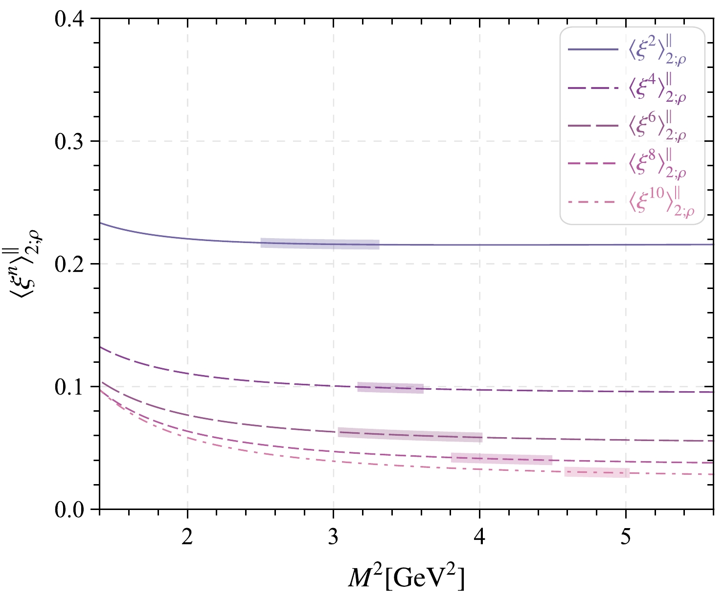

Figure 1

Figure 1.  (color online) ρ-meson leading-twist longitudinal DA moments $\langle \xi^n\rangle_{2;\rho}^\parallel$ with $n=(2,4,6,8,10)$ versus the Borel parameter $M^2$ and the corresponding Borel windows, where all input parameters are set as their central values.

DownLoad: Full-Size Img PowerPoint

Then, the values of ${\langle\xi^n\rangle_{2;\rho}^\parallel}|_\mu$ up to the 10th-order with four different scales $\mu =$ (1.0, 1.4, 2.0, 3.0) GeV and the second Gegenbauer moment $a_{2;\rho}^\parallel$ can be obtained, which are shown in Table 2. Here, we only calculate the values of the first five non-zero ξ-moments because, as shown in Ref. [57], these moments are sufficient to determine the behavior of the DA $\phi_{2;\rho}^\parallel(x,\mu)$. As a comparison, the other theoretical predictions obtained using QCD SRs [21−26], LQCD [27−30], AdS/QCD [31, 32], data fitting [35, 36], LFQM [39], and DSE [41] are also shown in Table 2. Our second moment is less than the QCD SR predictions in Ref. [21, 23, 26], the LQCD calculations [27−30], and DSE result [41] and larger than the QCD SR predictions in Refs. [24, 25] but very consistent with the value from QCD SRs in Ref. [22], the AdS/QCD prediction [31, 32], and the value extracted from the HERA data on diffractive ρ photoproduction [35, 36].

Table 2

Table 2.  Our predictions for the first five nonzero-order ξ-moments $\langle \xi^n\rangle _{2;\rho}^\parallel$ with $n=(2,4,6,8,10)$ and the second-order Gegenbauer moment $a_{2 \parallel}^{2;\rho}$ of the ρ-meson leading-twist longitudinal DA, compared with other theoretical predictions.

	$\mu {\rm /GeV }$	$\langle\xi^2\rangle_{2;\rho}^\parallel$	$\langle\xi^4\rangle_{2;\rho}^\parallel$	$\langle\xi^6\rangle_{2;\rho}^\parallel$	$\langle\xi^8\rangle_{2;\rho}^\parallel$	$\langle\xi^{10}\rangle_{2;\rho}^\parallel$	$a_{2 \parallel}^{2;\rho}$
This study	1.0	$0.220(6)$	$0.103(4)$	$0.0656(50)$	$0.0457(35)$	$0.0346(28)$	$0.059(18)$
This study	1.4	$0.217(5)$	$0.100(3)$	$0.0623(40)$	$0.0428(29)$	$0.0320(23)$	$0.051(16)$
This study	2.0	$0.215(5)$	$0.0986(31)$	$0.0603(35)$	$0.0411(25)$	$0.0304(20)$	$0.045(14)$
This study	3.0	$0.214(4)$	$0.0972(28)$	$0.0587(30)$	$0.0397(22)$	$0.0292(18)$	$0.041(13)$
QCD SRs [21]	1.0	−	−	−	−	−	$0.18(10)$
QCD SRs [22]	1.0	$0.227(7)$	$0.095(5)$	$0.051(4)$	$0.030(2)$	$0.020(5)$	−
QCD SRs [23, 26]	1.0	−	−	−	−	−	$0.15(7)$
QCD SRs [23, 26]	2.0	−	−	−	−	−	$0.10(5)$
QCD SRs [24]	1.0	$0.216(21)$	$0.089(9)$	$0.048(5)$	$0.030(3)$	$0.022(2)$	$0.047(58)$
QCD SRs [25]	2.0	$0.206(8)$	$0.087(6)$	−	−	−	$0.017(24)$
LQCD [27]	2.0	$0.237(36)(12)$	−	−	−	−	−
LQCD [28, 29]	2.0	$0.27(1)(2)$	−	−	−	−	−
LQCD [30]	2.0	−	−	−	−	−	$0.132(27)$
AdS/QCD [31, 32]	1.0	$0.228$	−	−	−	−	−
Data fitting [35, 36]	1.0	$0.227$	$0.105$	$0.062$	$0.041$	$0.029$	−
LFQM [39]	1.0	$0.21,0.19$	$0.09,0.08$	$0.05,0.04$	−	−	$0.02,-0.02$
DSE [41]	2.0	$0.23$	$0.11$	$0.066$	$0.045$	$0.033$	−

DownLoad: CSV

Show Table

By fitting our values of $\langle\xi^n\rangle_{2;\rho}^\parallel$ with $n = (2,4,6,8,10)$ shown in Table 2 using the least squares method (where the model parameters α and $\hat{a}_2$ are taken to be the fitting parameters, and for a specific fitting procedure, refer to Ref. [50]), the behavior of the ρ-meson leading-twist longitudinal DA can be obtained. The model parameters α and $\hat{a}_2$ of our DA and the corresponding $\chi^2_{\rm min}/n_d$ and goodness of fit $P_{\chi^2_{\rm min}}$ at several typical scales, such as $\mu = (1.0, 1.4, 2.0, 3.0)\; {\rm GeV}$ , are exhibited in Table 3. The curve of the ρ-meson leading-twist longitudinal DA is shown in Fig. 2. Other predictions in Refs. [25, 41, 46] are also shown for comparison. Our curve is closer to the asymptotic form. In addition, we use the TF model $\phi_{2;\rho}^{\parallel({\rm TF})}(x,\mu) = 6x(1-x) \Big[1 + a_{2\parallel}^{2;\rho} C_2^{3/2}(2x-1) + a_{4\parallel}^{2;\rho} C_4^{3/2}(2x-1) \Big]$ to fit our values of the ξ-moments of the ρ-meson leading-twist longitudinal DA shown in Table 2. The results indicate that the goodness of fits for the DSE model exhibited in Table 3 are close to those of the TF model at $\mu = 1\; {\rm GeV}$ but better than those of the TF model at $\mu = (1.4, 2.0, 3.0)\; {\rm GeV}$. For example, $a_{2\parallel}^{2;\rho} = 0.040$, $a_{4\parallel}^{2;\rho} = 0.054$, $\chi^2_{\rm min}/n_d = 0.657635/3$, and $P_{\chi^2_{\rm min}} = 0.88312$ at $\mu = 2\; {\rm GeV}$. The curve of the TF model $\mu = 2\; {\rm GeV}$ is also shown in Fig. 2. We find that the curve of the DSE model is smoother than that of the TF model. Thus, we use the DSE model instead of the TF model in this study.

Table 3

Table 3.  Model parameters α and $\hat{a}_2$ of our DA obtained by fitting using the least squares method and the corresponding $\chi^2_{\rm min}/n_d$ and goodness of fit $P_{\chi^2_{\rm min}}$ at several typical scales, such as $\mu = (1.0,~ 1.4,~ 2.0,~ 3.0)~ {\rm GeV}$.

μ	α	$\hat{a}_2$	$\chi^2_{\rm min}/n_d$	$P_{\chi^2_{\rm min}}$
$1.0$	$0.625$	$-0.516$	$0.957/3$	$0.812$
$1.4$	$0.678$	$-0.448$	$0.488/3$	$0.922$
$2.0$	$0.721$	$-0.398$	$0.259/3$	$0.968$
$3.0$	$0.709$	$-0.427$	$0.141/3$	$0.987$

DownLoad: CSV

Show Table

Figure 2

Figure 2.  (color online) Curve of our ρ-meson leading-twist longitudinal DA. As a comparison, the DA curves obtained using the DSEs [41], QCD SRs [25], algebraic model [46], asymptotic form, and fitting with the TF model are also shown.

DownLoad: Full-Size Img PowerPoint

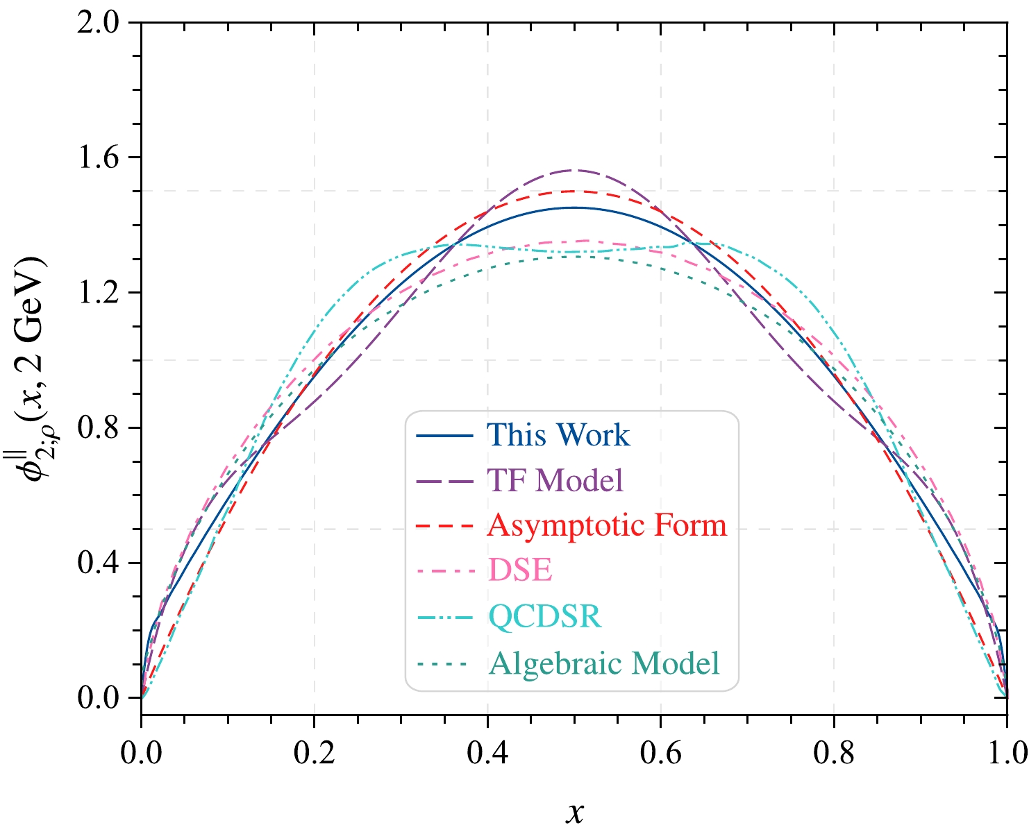
Furthermore, to calculate the $D\to \rho$ TFFs, the input parameters should be clarified. The current charm-quark mass is $m_c = 1.27\pm0.02\; {\rm GeV}$, and the D-meson mass is $m_D = 1.869\; {\rm GeV}$ [70]. Based on the three criteria for determining $s_0$ and $M^2$ in the LCSR approach, which can be found in our previous study [51], we have $s_0^{A_1} = 7.0\pm 0.1\; {\rm GeV}^2$, $s_0^{A_2}= 6.0\pm0.1\; {\rm GeV}^2$, $s_0^{V} = 7.0\pm 0.1 {\rm GeV}^2$, $M^2_{A_1} = 1.45\pm 0.05\; {\rm GeV}^2$, $M^2_{A_2} = 1.20\pm 0.05 \;{\rm GeV}^2$, and $M^2_{V} = 2.15\pm 0.05\; {\rm GeV}^2$. Then, the TFFs at the large recoil region, i.e., $A_{1,2}(0)$ and $V(0)$ , are present in Table 4. The uncertainties originate from the squared average for all the input parameters. In Table 4, the predictions from theoretical group and experimental collaborations, i.e., the CLEO collaboration [3], 3PSR [6], HQEFT [7, 8], RHOPM [9], QM [10, 11], LFQM [12], and HMχT [18], and lattice QCD predictions [19, 20] are presented. A comparison of all the results in Table 4 indicates that the TFFs of our prediction are consistent with those of many approaches within errors.

Table 4

Table 4.  $D\to \rho$ TFFs $A_{1,2}(q^2)$ and $V(q^2)$ at the large recoil region $q^2\simeq 0$. The errors are squared averages of all the mentioned error sources. As a comparison, we also present predictions from various other methods.

	$A_1(0)$	$A_2(0)$	$V(0)$
This study	$0.498^{+0.014}_{-0.012}$	$0.460^{+0.055}_{-0.047}$	$0.800^{+0.015}_{-0.014}$
CLEO2013 [3]	$0.56(1)^{+0.02}_{-0.03}$	$0.47(6)(4)$	$0.84(9)^{+0.05}_{-0.06}$
3PSR [6]	$0.5(2)$	$0.4(1)$	$1.0(2)$
HQETF [7]	$0.57(8)$	$0.52(7)$	$0.72(10)$
LCSR [8]	$0.599^{+0.035}_{-0.030}$	$0.372^{+0.026}_{-0.031}$	$0.801^{+0.044}_{-0.036}$
RHOPM [9]	0.78	0.92	1.23
QM-I [10]	0.59	0.23	1.34
QM-II [11]	0.59	0.49	0.90
LFQM [12]	$0.60(1)$	$0.47(0)$	$0.88(3)$
HMχT [18]	0.61	0.31	1.05
LQCD [19]	$0.45(4)$	$0.02(26)$	$0.78(12)$
LQCD [20]	$0.65(15){^{+0.24}_{-0.23}}$	$0.59(31){^{+0.28}_{-0.25}}$	$1.07(49)(35)$

DownLoad: CSV

Show Table

The ratios between different $D\to\rho$ TFFs, i.e., $r_2$ and $r_V$, are shown in Fig. 3. Here, the results from the CLEO collaboration [3], HMχT [18], LFQM [12], HQEFT [7], 3PSR [6], QM [10, 11], and CCQM [17] are presented for comparison. From the figure, we can reach the following conclusions:

Figure 3

Figure 3.  (color online) Predictions for the ratios $r_2$ and $r_V$ within uncertainties. The results from the CLEO collaboration [3], HMχT [18], LFQM [12], HQEFT [7], 3PSR [6], QM [10, 11], and CCQM [17] are presented for comparison.

DownLoad: Full-Size Img PowerPoint

● Our predictions within uncertainties are in the region of the CLEO collaboration results.

● In terms of the central value with respect to uncertainties, our results for $r_2$ agree with the QM, LFQM, 3PSR, and CCQM for theoretical predictions. $r_V$ agrees with the QM and 3PSR predictions.

● The uncertainties of our predictions are (12.9% ~ 14.4%) for $r_2$ and 4.4% for $r_V$, which indicates that this method can obtain applicable results in the confidence level. Because the predictions from the left-handed chiral current LCSR approach are mainly obtained at leading order for a strong coupling, we will consider the possible uncertainty/pollution from the axial-vector current in subsequent studies.

Using the resultant TFFs in the large recoil region, their behavior in the entire physical region, i.e., $q^2_{\rm phys.} \in [0, 1.18]\; \text{GeV}^2$ should be obtained. It is known that the LCSR predictions are suitable in low and intermediate momentum transfer. Therefore, a rapidly converging series based on $z(t)$-expansion is used to extrapolate in this study [73, 74],

The formula for $z(t)$ can be found in Ref. [73]. $F_i$ respects three TFFs, $A_{1,2}$ and V. The appropriate resonance masses are $m_{R,i}= 2.007\; {\rm GeV}$ for the TFF $V(q^2)$ with $J^P = 1^-$ and $m_{R,i}= 2.427\; {\rm GeV}$ for the TFFs $A_{1,2}(q^2)$ with $J^P = 1^+$. The parameters $a_k^i$ can be fixed by requiring $\Delta <$0.1%, where the parameter Δ is introduced to measure the quality of extrapolation, $\Delta={\sum_t|F_i(t)-F_i^{\rm fit}(t)|} / {\sum_t|F_i(t)|}\times 100$, where $t\in[0,1/40,\cdots,40/40]\times 0.8\; {\rm GeV}^2$. The $D\to \rho$ TFFs obtained in this study using LCSRs and the simple z-series expansion parameterization are shown in Fig. 4. The maximal momentum transfers of the LCSR calculation of the $D \to \rho$ TFFs are $A_1(q_{\rm max}) = 0.883^{+0.022}_{-0.019}$, $A_2(q_{\rm max}) = 0.611^{+0.102}_{-0.103}$ , and $V(q_{\rm max}) = 2.082^{+0.060}_{-0.059}$.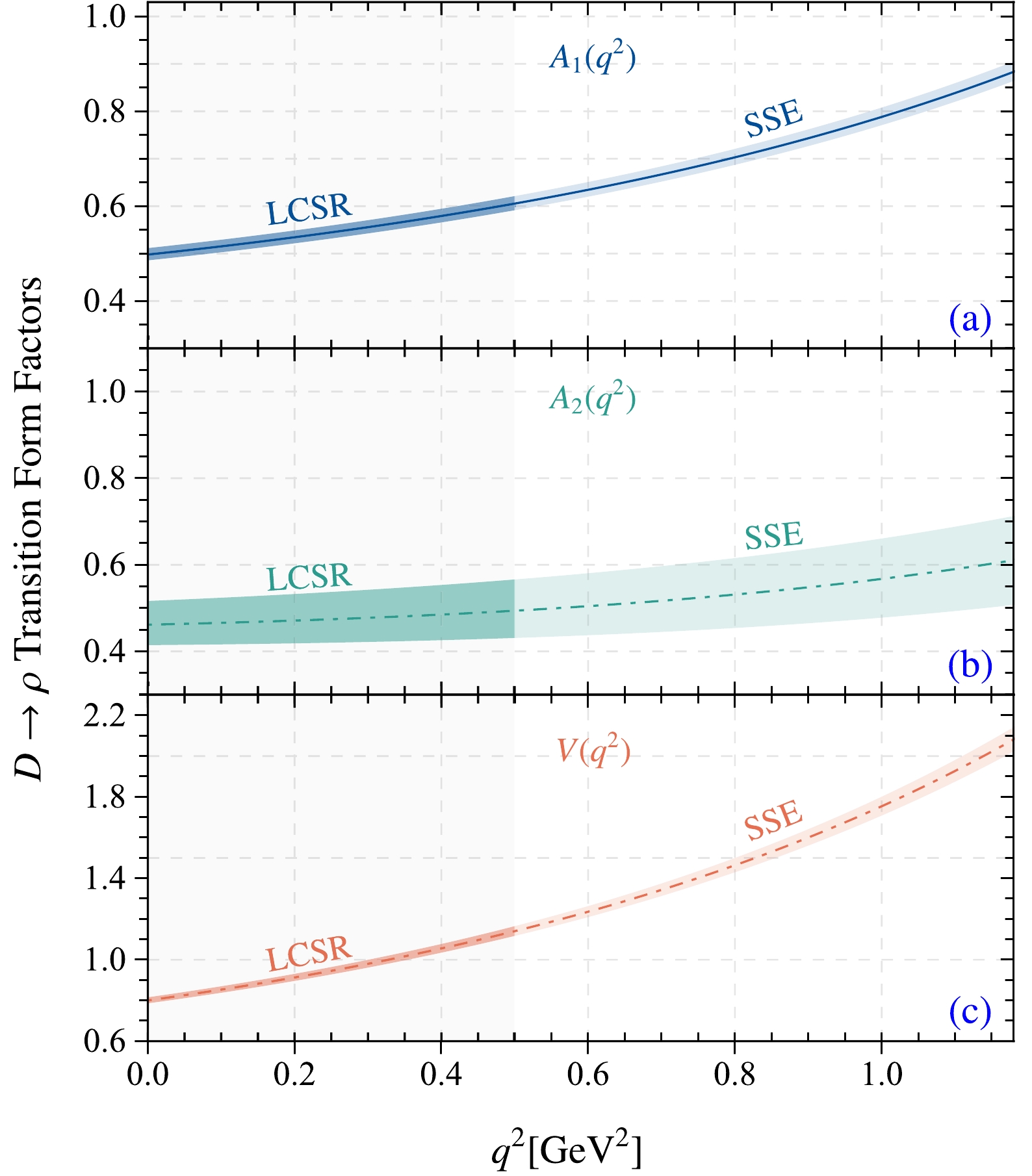

Figure 4

Figure 4.  (color online) Predictions for the $D\to \rho$ TFFs, where the darker bands are the results of this study using the LCSR approach, and the lighter bands are the predictions from simple z-series expansion parameterizations.

DownLoad: Full-Size Img PowerPoint

After obtaining the extrapolated TFFs of the transition $D\to\rho$, we find the CKM-independent total decay width $1/|V_{\rm cd}|^2 \times \Gamma$. Combining the ratio of the longitudinal/transverse and positive/negative helicity decay widths, we present the predictions in Table 5. The 3PSR [6], HQEFT [7], RHOPM [9], QM [10], LQCD [19], and LQCD [20] results are given for comparison. As shown in Table 5, there are large differences between the total decay widths from the different theoretical groups, and our results agree with the lattice results within uncertainties. Our predicted longitudinal/transverse helicity decay width agrees with those of HQEFT and LQCD within uncertainties, which is larger than 1. Our positive/negative helicity decay width agrees with that of the QM and LQCD within uncertainties.

Table 5

Table 5.  $|V_{cd}|$-independent total decay width $1/|V_{cd}|^2 \times \Gamma$, ratio for longitudinal/transverse and positive/negative helicity decay widths. For comparsion, other theoretical group predictions are also given.

	$1/|V_{\rm cd}|^2 \times \Gamma$	$\Gamma^{\rm L}/ \Gamma^{\rm T}$	$\Gamma^+/ \Gamma^-$
This study	$57.87^{+5.40}_{-5.13}$	$1.00^{+0.10}_{-0.11}$	$0.15^{+0.02}_{-0.01}$
3PSR [6]	$15.80\pm4.61$	$1.31\pm0.11$	$0.24\pm0.03$
HQEFT [7]	$71\pm14$	$1.17\pm0.09$	$0.29\pm0.13$
RHOPM [9]	$90.83$	0.91	0.19
QM [10]	$88.86$	1.33	0.11
LQCD [19]	$54.63\pm12.51$	$1.86\pm0.56$	0.16
LQCD [20]	71.75	1.10	0.18

DownLoad: CSV

Show Table

Lastly, the branching fractions for the two types of $D\to\rho\ell^+\nu_\ell$ semileptonic decays are calculated. The first is the $D^0$-type, including the $D^0 \to \rho^- e^+\nu_e$ and $D^0 \to \rho^- \mu^+\nu_\mu$ decays, for which the lifetime $\tau(D^0)= 0.410\pm 0.001$ ps should be used. The second is the $D^+$-type, including $D^+ \to \rho^0 e^+\nu_e$ and $D^+ \to \rho^0 \mu^+\nu_\mu$, associated with $\tau(D^+)= 1.033\pm 0.005$ ps [70]. The CKM matrix element $|V_{cd}| = 0.225\pm0.001$ [69]. We present the predictions in Table 6, where the two uncertainties mainly arise from the squared average of the theoretical input parameters and the experimental uncertainties from the D-meson lifetime. For comparison, the theoretical results from the 3PSR [6], HQEFT [7], narrow width approximation (NWA) [75] with the HQEFT [8] and LFQM [12] approaches, LCSR [8, 14], LFQM [13], CCQM [17], chiral unitarity approach (χUA) [76], RQM [77], HMχT [18], ISGW2 [78] and experimental results from the BESIII collaboration [1, 2] and CLEO collaboration prediction in 2013 [3] and 2005 [4] are also given. The results show that:

Table 6

Table 6.  Branching ratios of the semileptonic decays $D^0\to \rho^- \ell^+ \nu_\ell$ and $D^+ \to \rho^0 \ell^+ \nu_\ell$ (in units of $10^{-3}$). For comparison, we also present the results from experimental collaborations and theoretical groups.

Decay Mode	$D^0\to \rho^- e^+ \nu_e$	$D^+ \to \rho^0 e^+ \nu_e$	$D^0\to \rho^- \mu^+ \nu_\mu$	$D^+ \to \rho^0 \mu^+ \nu_\mu$
This study	$1.825^{+0.170}_{-0.162}\pm 0.004$	$2.299^{+0.214}_{-0.204}\pm 0.011$	$1.816^{+0.168}_{-0.160}\pm 0.004$	$2.288^{+0.212}_{-0.201}\pm 0.011$
BESIII [1]	−	−	$1.35\pm0.09\pm0.09$	−
BESIII [2]	$1.445\pm0.058\pm0.039$	$1.860\pm0.070\pm0.061$	−	−
CLEO2013 [3]	$1.77\pm0.12\pm0.10$	$2.17\pm0.12^{+0.12}_{-0.22}$	−	−
CLEO2005 [4]	$1.94\pm0.39\pm0.13$	$2.1\pm0.4\pm0.1$	−	−
3PSR [6]	$0.5\pm0.1$	−	−	−
HQEFT [7]	$1.4\pm0.3$	−	−	−
LCSR [8]	$1.81^{+0.18}_{-0.13}$	$2.29^{+0.23}_{-0.16}$	$1.73^{+0.17}_{-0.13}$	$2.20^{+0.21}_{-0.16}$
NWA [75]+HQEFT [8]	$1.67\pm0.27$	$2.16\pm0.36$	−	−
NWA [75]+LFQM [12]	$1.73\pm0.07$	$2.24\pm0.09$	−	−
LFQM [13]	−	−	$1.7\pm0.2$	−
LCSR [14]	$1.74\pm0.25$	$2.25\pm0.32$	$1.65\pm0.23$	$2.14\pm0.30$
CCQM [17]	1.62	2.09	1.55	2.01
HMχT [18]	2.0	2.5	−	−
χUA [76]	1.97	2.54	1.84	2.37
RQM [77]	1.96	2.49	1.88	2.39
ISGW2 [78]	1.0	1.3	−	−

DownLoad: CSV

Show Table

● The results obtained using our left-handed chiral LCSR approach are consistent with those obtained using other LCSRs within uncertainties.

● Our current results are consistent with those of the CLEO collaboration but are larger than the BESIII collaboration predictions.

● Our results are consistent with those of other theoretical groups, such as the NWA, LFQM, HQEFT, χUA, RQM, and HMχT, but have a smaller gap when compared with the 3PSR, HQEFT, χUA, and ISGW2 results.

IV. SUMMARY

• I. INTRODUCTION
• II. THEORETICAL FRAMEWORK
• III. NUMERICAL ANALYSIS
• IV. SUMMARY
• ACKNOWLEDGMENTS

In the framework of BFT with the QCD SR approach, we calculate the ξ-moments of the ρ-meson leading twist longitudinal DA. Because the zeroth ξ-moment cannot be normalized in the entire Borel region, a new SR formula for the ξ-moment is given in Eq. (2). The results up to the tenth order with the scale $\mu = (1.0,1.4,2.0.3.0)\; {\rm GeV}^2$ are presented in Table 2, where the results from other theoretical group are also given. Next, we present the $D\to \rho$TFFs in the large recoil region, i.e., $A_1(0),~ A_2(0)$, and $V(0)$, in Table 4 and the ratio $r_{2,V}$ in Fig. 3, which indicate that our results are reasonable and consistent with those of many approaches within errors. Subsequently, we calculate the $|V_{cd}|$-independent total decay width and the ratio for the longitudinal/transverse and positive/negative helicity decay width results and present them in Table 5. A detail discussion comparing our results with other predictions is presented. Finally, we show the branching fraction of the two types of $D\to\rho\ell^+\nu_\ell$ semileptonic decays in Table 6. In the near further, we hope that more accurate data will be reported and more theoretical results will be given to explain the gaps between different approaches.

ACKNOWLEDGMENTS

• I. INTRODUCTION
• II. THEORETICAL FRAMEWORK
• III. NUMERICAL ANALYSIS
• IV. SUMMARY
• ACKNOWLEDGMENTS

We are grateful for the referee's valuable comments and suggestions.

1Chiral current LCSR approach will be introduced in the next section of this paper

References