Possible bias of the constraints on the Hubble constant owing to the quasi-Gaussian distribution of DM_IGM in fast radio bursts

Fast radio bursts (FRBs) are bright and energetic radio pulses characterized by millisecond durations that primarily originate from extragalactic sources [1–4]. The first FRB signal, now named FRB 010724, was discovered by Lorimer et al. [5] in 2007 from the 2001 archive data of the Parkes 64-m telescope. In 2013, Thornton et al. [6] discovered several similar signals; thereafter, FRBs began to attract people's interest. FRBs can be generally categorized into two classes: repeaters and non-repeaters. However, it is unclear whether there are essential differences between them. The first discovered repeating FRB was FRB 121102, which is extremely active and can repeat over a thousand times in $ \sim 60 $ hours [7]. Other repeating FRBs might repeat only two or three times [8]. FRBs also have a high occurrence rate across the full sky. To date, hundreds of FRBs have been discovered by various telescopes [1, 9]. FRB 200428 confirmed that at least some FRBs may originate from magnetars, but there is still no consensus on the origin of most FRBs. The large dispersion measures (DMs) show that the majority of FRBs have an extragalactic origin, with only one FRB confirmed to come from the Milky Way [10]. The localization of the host galaxy and the direct measurement of redshift confirm that they have an extragalactic origin [11–13], thus making FRBs a useful tool to study the universe.

Recently, the Hubble tension problem, i.e., the contradiction between the Hubble constant values measured from the cosmic microwave background (CMB) and Type Ia supernovae (SNe Ia), called people's attention [14–17]. New probes for the universe are necessary to resolve the Hubble tension problem, and FRBs may potentially be such probes. The high energy of FRBs enables their detection at high redshift, and their high DM also makes them useful cosmological probes. For instance, Macquart et al. [18] used FRBs to constrain the missing baryons in the universe. Gao et al. [19] used FRB/GRB systems to constrain the dark energy. Zhao et al. [20] used simulated FRB data to break the parameter degeneracies inherent to the CMB data. Qiu et al. [21] combined simulated FRB data with current CMB data to constrain the holographic dark energy (HDE) and Ricci dark energy (RDE) models. Zhao et al. [22] used unlocalized FRB data to constrain the Hubble constant. Zhang et al. [23] investigated how the upcoming FRB observations with the Square Kilometre Array (SKA) can help advance cosmology, and showed that $ 10^6 $ FRB data can tightly constrain the dark-energy equation of state parameters and the baryon density $ \Omega_{\rm{b}}h $. Bhattacharya et al. [24] used FRBs to explore the reionization history of the universe. Lin and Sang [25] used FRBs to test the anisotropy of the universe. Wu et al. [26] used FRBs to constrain the Hubble constant. Li et al. [27] used strongly lensed FRBs to constrain cosmological parameters such as the Hubble constant and the curvature of the Universe. Pearson et al. [28] pointed out that strongly lensed repeating FRBs can be used to search for gravitational waves.

There are some key issues in using FRBs as cosmological probes. First, although hundreds of FRBs have been measured, only a few of them have been subjected to a direct measurement of redshift. Fortunately, many more FRBs are expected to be detected in the future by telescopes such as the Canadian Hydrogen Intensity Mapping Experiment (CHIME) and the Five-hundred-meter Aperture Spherical Telescope (FAST), and some of them are expected to be subjected to a direct redshift measurement [29, 30]. Second, the DM contribution from the host galaxy ($ \rm DM_{host} $) is not fully understood, and it may significantly differ among FRBs. Therefore, it is difficult to precisely model the $ \rm DM_{host} $ term. Some previous studies assumed that the $ \rm DM_{host} $ term accommodates the evolution of the star formation rate history; hence, it evolves with redshift [31]. However, Lin et al. [32] found that there is no strong evidence for the redshift evolution of $ \rm DM_{host} $ within the present data. A more reasonable approach is to consider the probability distribution of $ \rm DM_{host} $ and marginalize over it. Based on theoretical considerations and numerical simulations, Macquart et al. [18] and Zhang et al. [33] showed that $ \rm DM_{host} $ follows a log-normal distribution. Finally, owing to the fluctuation of the matter density, the DM contribution from the intergalactic medium ($ \rm DM_{IGM} $) may significantly deviate from the mean value. Therefore, using the mean value to estimate $ \rm DM_{IGM} $ may strongly bias the results. A usual approach is to treat $ \rm DM_{IGM} $ as a Gaussian distribution centered on the mean value. The Gaussian distribution is useful owing to the Gaussianity of structures on large scales; however, a large skew may emerge from several large-scale structures. Considering this, Macquart et al. [18] proposed a quasi-Gaussian distribution of $ \rm DM_{IGM} $ based on hydrodynamic simulations and theoretical motivation. Different treatments of $ \rm DM_{IGM} $ may affect the constraint on cosmological parameters.

In this study, we used 18 well-localized FRBs to constrain the Hubble constant $ H_0 $. The probability distributions of $ \rm DM_{IGM} $ and $ \rm DM_{host} $ were considered, and the free parameters that govern the probability distributions were constrained simultaneously with the Hubble constant. The rest of this paper is organized as follows. Sec. II introduces the Bayesian method used to constrain cosmological parameters. Sec. III reports on the observational data and constraining results. Sec. IV analyzes the Monte Carlo simulations performed to check the validity of the proposed method and compares the impacts of different probability distributions of $ \rm DM_{IGM} $. Finally, a discussion and conclusions are provided in Sec. V.

When an FRB signal travels from the host galaxy to the Earth, it experiences a time delay due to the interaction of electromagnetic waves with free electrons. This time delay depends on the frequency of the electromagnetic waves. Measuring the time delay between photons of different frequencies allows determining the number density of electrons integrated along the wave path; this is referred to as the dispersion measure (DM). The total dispersion measure of an extragalactic FRB can be generally separated into four components [18],

where $ \rm DM_{MW} $ comes from the contribution of Galactic interstellar medium, which can be estimated from Galactic electron density models such as the NE2001 model [34]. The $ \rm DM_{halo} $ term is the contribution from the Galactic halo, which is not fully constrained yet; Prochaska et al. [35] provided an estimated value of approximately $ \rm 50- 100\ pc\ cm^{-3} $. In this study, we followed Macquart et al. [18] and assumed $ \rm DM_{halo}=50\ pc\ cm^{-3} $. The $ \rm DM_{host} $ term is the contribution from the host galaxy, and the factor $ 1+z $ arises from the cosmic expansion. The $ \rm DM_{IGM} $ term is the contribution from the intergalactic medium; it carries the information of the universe. Other studies also mentioned the $ \rm DM_{source} $ term [3, 4, 23], which represents the DM contribution from the immediate environment of the source. The $ \rm DM_{source} $ term is highly dependent on the source environment of each FRB, which is not fully understood yet. The value of $ \rm DM_{source} $ is usually smaller than the error of $ \rm DM_{host} $ and $ \rm DM_{IGM} $ [36]. Therefore, we ignored the $ \rm DM_{source} $ term in this study. The $ \rm DM_{MW} $ and $ \rm DM_{halo} $ terms can be subtracted from the total observed $ {\rm{DM}} $, leaving behind the extragalactic $ \rm DM $, which is defined as

In the flat $ \rm \Lambda CDM $ model, the average value of the $ \rm DM_{IGM} $ term can be expressed as [37, 38]

where $ H_0 $ is the Hubble constant, $ \rm \Omega_b $ is the cosmic baryon mass density, $ \Omega_m $ is the matter density, and $ \Omega_{\Lambda} $ is the vacuum energy density of the Universe; c, G, and $ m_p $ are three constants that represent the speed of light in vacuum, the Newtonian gravitational constant, and the mass of proton, respectively; $f_e= Y_{\rm{H}} X_{e,{\rm{H}}}+Y_{\rm{He}}X_{e,{\rm{He}}}/2$ denotes the extent of ionization progress of hydrogen and helium, where $ Y_{\rm{H}}=0.75 $ and $ Y_{\rm{He}}=0.25 $ are the hydrogen and helium mass fractions, respectively; $ X_{e,{\rm{H}}} $ and $ X_{e,{\rm{He}}} $ are the corresponding ionization fractions. Given that both hydrogen and helium are expected to be fully ionized at $ z \leq 3 $ [39, 40], we set $ X_{e,{\rm{H}}}=X_{e,{\rm{He}}}=1 $; $ f_{\rm{IGM}} $ is the fraction of baryon mass in IGM.

Note that Eq. (3) only describes the mean value of $ \rm DM_{IGM} $. Its real value is associated with large-scale matter density fluctuations and may vary around the mean value. Usually, a Gaussian distribution is used to describe $ \rm DM_{IGM} $ [41–43]. However, theoretical results and numerical simulations show that the probability distribution of $ \rm DM_{IGM} $ can be modeled using a quasi-Gaussian distribution [18, 44],

where $ \rm \Delta \equiv DM_{IGM}/\langle DM_{IGM} \rangle $, $ \rm \sigma_{IGM} $ is the effective standard deviation, and α and β are related to the inner density profile of gas in haloes. Hydrodynamic simulations show that $ \alpha=\beta=3 $ provides the best fit to the model [18, 44]; hence, we fixed these two parameters. We also followed Macquart et al. [18] to parameterize the effective standard deviation as $ {\rm{\sigma_{IGM}}} = Fz^{-1/2} $, where F is a free parameter and z is the redshift of the FRB source. Here, A is a normalization constant, and $ C_0 $ is chosen to ensure that the mean of this distribution is unity. Note that the distribution of $ \rm DM_{IGM} $ is a function of z, implying that A and $ C_0 $ vary with z.

The $ \rm DM_{host} $ term may range from tens to hundreds of $ \rm pc\ cm^{-3} $. For example, Xu et al. [45] estimated that the $ \rm DM_{host} $ of FRB20201124A can range from 10 to 310 $ \rm pc\ cm^{-3} $, while Niu et al. [46] estimated that the value of $ \rm DM_{host} $ for FRB20190520B can reach 900 $ \rm pc\ cm^{-3} $. To account for the large variation of $ \rm DM_{host} $, it is often modeled with a log-normal distribution [18, 33],

where μ and $ \sigma_{\rm{host}} $ are the mean and standard deviation of $ \rm \ln{DM_{host}} $, respectively. This log-normal distribution allows for the appearance of large values of $ \rm DM_{host} $. Generally, both μ and $ \sigma_{\rm{host}} $ might be redshift-dependent. However, Zhang et al. [33] showed that, for non-repeating bursts, they do not vary significantly with redshift. Lin et al. [32] also proved that there is no strong evidence for redshift evolution of $ \rm DM_{host} $ within the present data. Hence, we followed Macquart et al. [18] and treated them as two constants.

Given that it is challenging to separate the terms $ \rm DM_{IGM} $ and $ \rm DM_{host} $, we introduce the probability distribution of the extragalactic $ \rm DM $ as [18]

If a large sample of well-localized FRBs is observed, the joint likelihood function can be expressed as

where N is the number of FRBs. According to the Bayesian theorem, the posterior probability density function of the free parameters is given by

where $ P_0 $ is the prior probability function of the parameters.

To date, over 30 published well-localized extragalactic FRBs have identified host galaxies and well-measured redshifts ¹. Among them, FRB20200120E, FRB20190614D, FRB20190520B, and FRB 20220319D are excluded. FRB20200120E is so close to the Milky Way that the peculiar velocity dominates the Hubble flow, resulting in a negative spectroscopic redshift of $ z=-0.001 $ [47, 48]. FRB20190614D only has a photometric redshift of $ z\approx 0.6 $ [49], with no available spectroscopic redshift. The value of $ {\rm{DM_{host}}} $ for FRB20190520B is estimated to be as large as $ 900\ \rm pc\ cm^{-3} $ [46], which is much larger than the value of normal FRBs. FRB20220319D is also excluded owing to its total DM, which is lower than $ \rm DM_{MW} $ [50]. The remaining 35 FRBs have well-measured spectroscopic redshifts, and their main properties are listed in Table 1. These FRBs were used to constrain the cosmological parameters in this study.

FRBs	RA	Dec	$ {\rm DM_{obs}} $/($ ^{\circ} $)	$ {\rm DM_{MW}} $/$ {\rm pc cm^{-3}} $	$ {\rm DM_E} $/$ {\rm pc cm^{-3}} $	$ z_{\rm sp} $/$ {\rm pc cm^{-3}} $	Reference
20121102A	82.99	33.15	557.00	157.60	349.40	0.1927	Chatterjee et al. [12]
20171020A	22.15	−19.40	114.10	38.00	26.10	0.0087	Li et al. [51]
20180301A	93.23	4.67	536.00	136.53	349.47	0.3305	Bhandari et al. [52]
20180916B	29.50	65.72	348.80	168.73	130.07	0.0337	Marcote et al. [53]
20180924B	326.11	−40.90	362.16	41.45	270.71	0.3214	Bannister et al. [54]
20181030A	158.60	73.76	103.50	40.16	13.34	0.0039	Bhardwaj et al. [55]
20181112A	327.35	−52.97	589.00	41.98	497.02	0.4755	Prochaska et al. [56]
20190102C	322.42	−79.48	364.55	56.22	258.33	0.2913	Macquart et al. [18]
20190523A	207.06	72.47	760.80	36.74	674.06	0.6600	Ravi et al. [57]
20190608B	334.02	−7.90	340.05	37.81	252..24	0.1178	Macquart et al. [18]
20190611B	320.74	−79.40	332.63	56.60	226.03	0.3778	Macquart et al. [18]
20190711A	329.42	−80.36	592.60	55.37	487.23	0.5217	Macquart et al. [18]
20190714A	183.98	−13.02	504.13	38.00	416.13	0.2365	Heintz et al. [58]
20191001A	323.35	−54.75	507.90	44.22	413.68	0.2340	Heintz et al. [58]
20191228A	344.43	−29.59	297.50	33.75	213.75	0.2432	Bhandari et al. [52]
20200430A	229.71	12.38	380.25	27.35	302.90	0.1608	Bhandari et al. [52]
20200906A	53.50	−14.08	577.80	36.19	491.61	0.3688	Bhandari et al. [52]
20201124A	77.01	26.06	413.52	126.49	237.03	0.0979	Fong et al. [59]
20210405I	255.34	−48.48	565.17	468.18	46.99	0.066	Driessen et al. [60]
20210410D	326.09	−78.68	572.62	56.20	466.45	0.1415	Caleb et al. [61]
20210603A	10.27	21.23	500.15	40.00	410.15	0.1772	Cassanelli et al. [62]
20211127A	199.81	−18.84	234.83	41.75	143.08	0.0496	Khrykin et al. [63]
20211212A	157.35	1.36	206.00	38.29	117.71	0.0713	Khrykin et al. [63]
20220207C	310.20	72.88	262.38	74.99	137.39	0.0430	Law et al. [64]
20220307B	350.87	72.19	499.27	119.82	329.45	0.2481	Law et al. [64]
20220310F	134.72	73.49	462.24	45.07	367.17	0.4780	Law et al. [64]
20220418A	219.10	70.10	623.25	36.49	536.76	0.6220	Law et al. [64]
20220506D	318.04	72.83	396.97	82.88	264.09	0.3004	Law et al. [64]
20220509G	282.67	70.24	269.53	55.36	164.17	0.0894	Law et al. [64]
20220825A	311.98	72.58	651.24	77.26	523.98	0.2414	Law et al. [64]
20220912A	347.27	48.71	220.7	120.44	50.26	0.0771	Zhang et al. [65]
20220914A	282.06	73.34	631.28	54.38	526.9	0.1139	Law et al. [64]
20220920A	240.26	70.92	314.99	39.62	225.37	0.1582	Law et al. [64]
20221012A	280.80	70.52	441.08	53.69	337.39	0.2847	Law et al. [64]
20221022A	48.63	86.87	116.84	60.12	6.72	0.0149	Mckinven et al. [66]

Table 1.  Properties of the Host/FRB catalog. Column 1: FRB name; Columns 2 and 3: right ascension and declination of the FRB source on the sky; Column 4: observed DM; Column 5: DM of the Milky Way ISM calculated using the NE2001 model; Column 6: extragalactic DM calculated by subtracting $ {\rm{DM_{\rm MW}}} $ and $ {\rm{DM_{\rm halo}}} $ from the observed $ {\rm{DM_{\rm obs}}} $, assuming $ {\rm{DM_{\rm halo}}}=50\; {\rm{pc\; cm^{-3}}} $for the Milky Way halo; Column 7: spectroscopic redshift; Column 8: references.

We employed Monte Carlo Markov Chain (MCMC) analysis to constrain $ H_0 $ and three free parameters ($ e^{\mu},\ \sigma_{\rm{host}}, F $) from the probability functions of $ \rm DM_{host} $ and $ \rm DM_{IGM} $. We used $ e^{\mu} $ instead of μ as a free parameter because $ e^{\mu} $ directly represents the median value of $ \rm DM_{host} $. For $ f_{\rm{IGM}} $, there is no precise constraint yet. It may slowly increase with redshift [67]; Li et al. [31] parameterized it as $ f_{\rm{IGM}}=f_{{\rm{IGM}},0}(1+\alpha z/(1+z)) $. However, there is no strong evidence showing that $ f_{\rm{IGM}} $ increases with redshift in the current FRB data [68]. To be conservative, we assumed that $ f_{\rm{IGM}} $ follows a uniform distribution $ U $ (0.747, 0.913) and marginalized over it [26]. Additionally, we set $ \Omega_b h^2 = 0.0224 $ and $ \Omega_m = 0.315 $ according to Planck 2018 results [69]. The posterior probability density functions of the free parameters were calculated using the publicly available Python code emcee [70]. Based on previous results [18, 71], flat priors were applied to the four parameters as follows: $ H_0 \in U(0,100)\; {\rm{km\; s^{-1}}\; Mpc^{-1}} $, $e^{\mu} \in U(20, 200) {\rm{\ pc\ cm^{-3}}}$, $ \sigma_{\rm{host}} \in U(0.2,2) $, and $ F \in U(0.01,0.5) $.

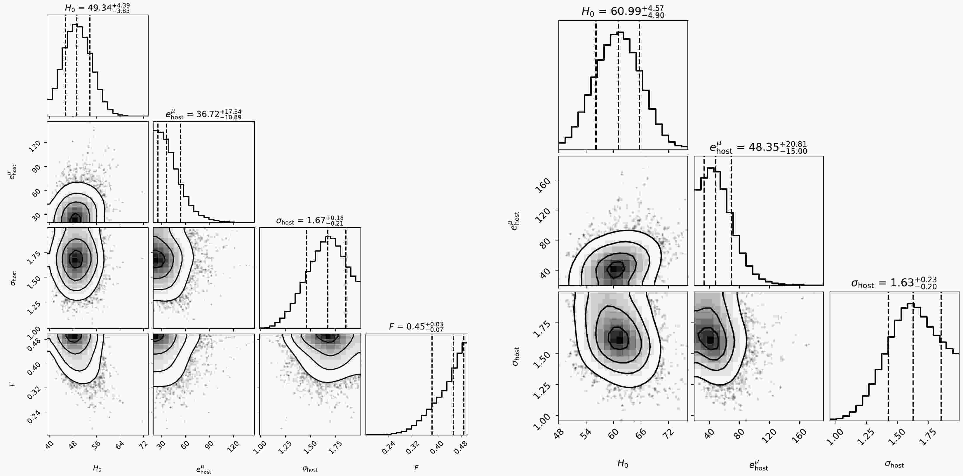
The 2D marginalized posterior distributions and $ 1-3\ \sigma $ confidence contours of the four parameters are plotted in the left panel of Fig. 1. It is evident that only the parameters $ H_0 $ and $ \sigma_{\rm{host}} $ are tightly constrained, while the other two parameters, i.e., $ e^{\mu} $ and F, are not well-constrained. A possible reason is that the FRB sample is not large enough to simultaneously constrain a model with too many free parameters. A notable feature is that the best-fitting value of the Hubble constant is $H_0= 49.34^{+4.39}_{-3.83}\;\; {\rm{km\; s^{-1}}\; Mpc^{-1}}$, which is much lower than the Planck 2018 value. This discrepancy may be caused by the correlation between parameters. As can be seen from the contour plot, $ H_0 $ seems to be positively correlated with $ e^{\mu}_{\rm{host}} $ and negatively correlated with F.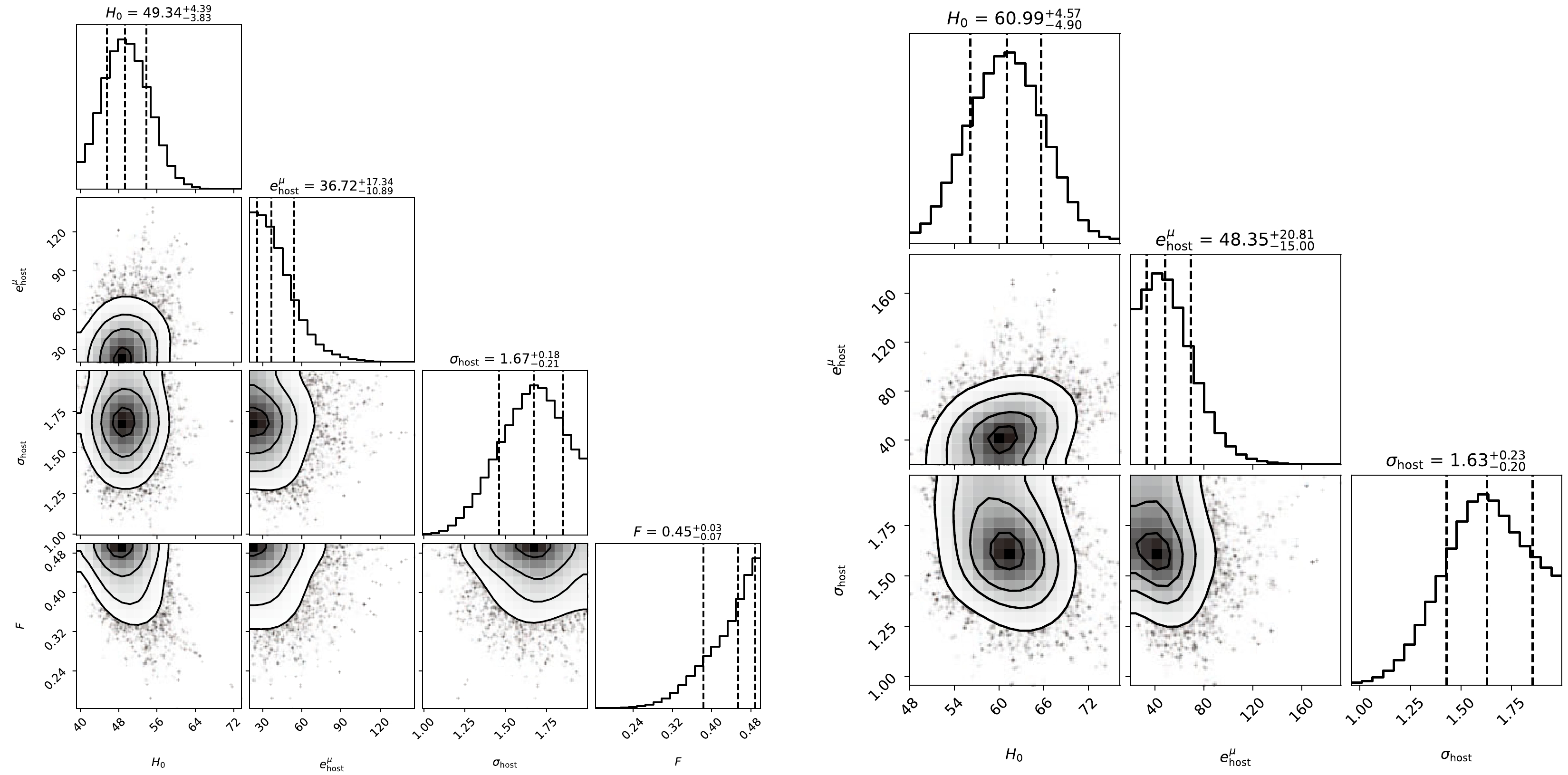

Figure 1.  Constraints on the four free parameters ($ H_0,\ e^{\mu},\ \sigma_{\rm{host}} $, F) and three free parameters ($ H_0,\ e^{\mu},\ \sigma_{\rm{host}} $) using the 35 FRBs samples. The black-dashed lines from left to right in each subfigure represents the 16%, 50%, and 84% quantiles of the distribution, respectively. The contours from the inner to outer represent $ 1\sigma $, $ 2\sigma $, and $ 3\sigma $ confidence regions, respectively. For simplicity, units are omitted in this figure.

Several previous studies suggest that a suitable value for the parameter F is approximately $ F=0.2 $, or even smaller for $ z\leq 1 $ [72, 73]. However, our four-parameter fit from the FRB sample indicates that a larger value of F may be more suitable, although it cannot be tightly constrained. This discrepancy might introduce bias to the other parameters. To address this issue, we fixed $ F = 0.2 $ while keeping the other three parameters $ (H_0,\ e^{\mu},\ \sigma_{\rm{host}}) $ free. The corresponding 2D marginalized posterior distributions and $ 1-3\ \sigma $ confidence contours of the three parameters are presented in the right panel of Fig. 1. Note that both $ H_0 $ and $ \sigma_{\rm{host}} $ are well-constrained, and the parameter $ e^{\mu}_{\rm{host}} $ is also constrained but with a relatively small value. The best-fitting Hubble constant, $H_0=60.99^{+4.57}_{-4.90} {\rm{km\; s^{-1}}\; Mpc^{-1}}$, is notably larger than that from the four-parametric fit. However, the median value of the Hubble constant is still relatively lower than the Planck 2018 value. A possible explanation is that the FRB sample is not large enough to provide a robust result. The results for both parameters from the probability functions of $ \rm DM_{host} $ are $ e^{\mu}_{\rm{host}}=48.35^{+20.81}_{-15.00} {\rm{\ pc\ cm^{-3}}} $ and $ \sigma_{\rm{host}}=1.63^{+0.23}_{-0.20} $, both of which have relatively large uncertainties.

With the progress of observational techniques, more and more FRBs are expected to be detected, and a fraction of them can be well-localized. Therefore, it is interesting to assess the constraining capability of a large sample of FRBs across a wide redshift range. To this end, we performed Monte Carlo simulations to investigate the efficiency of the proposed method.

The intrinsic redshift distribution of FRBs is still unclear because of the small well-localized sample. Li et al. [31] assumed that FRBs have a constant comoving number density but with a Gaussian cutoff. Zhang et al. [38] argued that the redshift distribution of FRBs is expected to be related with cosmic star formation rate (SFR), or influenced by the compact star merger but with an additional time delay. In this study, we adopted the SFR-related model, in which the probability density function takes the form [38]

where $D_c(z)= \int_0^z \dfrac{c{\rm d}z}{H(z)}$ represents the comoving distance, c denotes the speed of light, $ H(z) $ represents the Hubble expansion rate, and SFR takes the form [74]

where $ a=3.4,\ b=-0.3,\ c=-3.5,\ B=5000,\ C=9 $, and $ \eta = -10 $.

We simulated a set of mock FRB samples to constrain the parameters. The simulations were performed according to the flat $ \rm \Lambda CDM $ model with Planck 2018 results [69]. The fiducial parameters were set as $F=0.2, \ f_{\rm{IGM}}=0.83, \; \ e^{\mu}=100{\rm\ pc\ cm^{-3}}$, and $ \sigma_{\rm{host}}=1.0 $. The simulation procedures were as follows. First, a certain number of redshifts were randomly drawn from Eq. (9), with $ z_{\rm{max}} $ set to $ 3.0 $. Subsequently, the same number of Δ values were randomly drawn from Eq. (4). The average $ \rm \langle DM_{IGM}(z)\rangle $ was calculated using Eq. (3), and $ \rm DM_{IGM} $ was obtained for each redshift as $ \Delta \times \langle {\rm{DM_{IGM}}}(z)\rangle $. Next, the same number of $ \rm DM_{host} $ values were randomly drawn from Eq. (5), and $ \rm DM_{E} $ was calculated from Eq. (2). A sample of mock FRBs $ (z_i, {\rm{DM_{E,\it i}}}) $ was also part of the simulations.

We used these mock FRBs to constrain the four parameters ($ H_0 $, $ e^\mu $, $ \sigma_{\rm{host}} $, F) using the same method described above. The corresponding contour plots constrained from $ N=100 $ mock FRBs are shown in the left panel of Fig. 2. Note that only the parameter $ H_0 $ can be tightly constrained. Note also that the parameter $ H_0 $ fails to recover the fiducial value within 1σ uncertainty.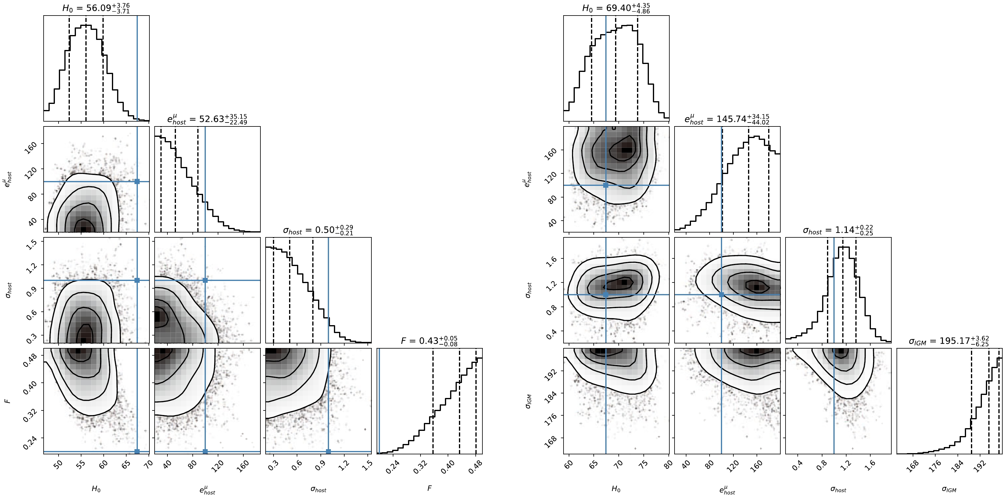

Figure 2.  (color online) Constraints on the four free parameters ($ H_0 $, $ e^\mu $, $ \sigma_{\rm{host}} $, F) using 100 mock FRBs with quasi-Gaussian (left panel) and Gaussian (right panel) distributions of $ \rm DM_{IGM} $. The blue lines represent the fiducial values. The black-dashed lines from left to right in each subfigure represents the 16%, 50%, and 84% quantiles of the distribution, respectively. The contours from the inner to outer represent $ 1\sigma $, $ 2\sigma $, and $ 3\sigma $ confidence regions, respectively. For simplicity, units are omitted in this figure.

For comparison, we also conducted MCMC analysis using a Gaussian distribution of $ \rm DM_{IGM} $. In this case, the method is similar to that of the quasi-Gaussian distribution, with the primary difference being the replacement of the distribution function of $ \rm DM_{IGM} $ (i.e., Eq. (4)) with the Gaussian distribution $ \mathcal{G}(\langle {\rm{DM_{IGM}}} \rangle, \sigma_{\rm{IGM}}) $ for the generation of mock FRBs samples and in the joint likelihood function. In this simulation, the fiducial value of $ \sigma_{\rm{IGM}} $ was set to $ 100{\rm{\ pc\ cm^{-3}}} $ [41, 42]. In the MCMC analysis, $ \sigma_{\rm{IGM}} $ was treated as a free parameter, replacing the parameter F of the quasi-Gaussian case. The prior of $ \sigma_{\rm{IGM}} $ was $ U(0,200)\ {\rm{pc\ cm^{-3}}} $. We employed mock FRBs generated with a Gaussian distribution of $ \rm DM_{IGM} $ to constrain the four parameters ($ H_0 $, $ e^\mu $, $ \sigma_{\rm{host}} $, $ \sigma_{\rm{IGM}} $). The corresponding contour plots constrained from $ N=100 $ mock FRBs are shown in the right panel of Fig. 2. Note that with the Gaussian distribution of $ \rm DM_{IGM} $, the parameters $ H_0 $ and $ \sigma_{\rm{host}} $ can properly recover their fiducial values. However, the other two parameters ($ e^{\mu} $, $ \sigma_{\rm{IGM}} $), especially $ \sigma_{\rm{IGM}} $, cannot be tightly constrained, showing a strong bias with respect to the fiducial value.

Given that the best-fitting value of F is much larger than the expected one, we fixed $ F = 0.2 $ to explore whether the results could be improved. The corresponding contour plots constrained from $ N=100 $ mock FRBs with quasi-Gaussian distribution of $ \rm DM_{IGM} $ are shown in the left panel of Fig. 3. With 100 mock FRBs, we obtained a well-constrained Hubble constant, providing a more precise result compared to that with 35 real FRBs. The other two parameters, i.e., $ e^\mu $ and $ \sigma_{\rm{host}} $, were also well-constrained but exhibited a relatively large uncertainty. Regardless of this large uncertainty, the three parameters can properly recover the fiducial values within $ 1\sigma $ uncertainty. However, with a thousand repetitions, each involving a sample of 100 mock FRBs, nearly half of the estimates for $ e^{\mu} $ and $ \sigma_{\rm{host}} $ could not be well constrained. Therefore, caution is advised when discussing the results of $ e^{\mu} $ and $ \sigma_{\rm{host}} $ in real-world situations.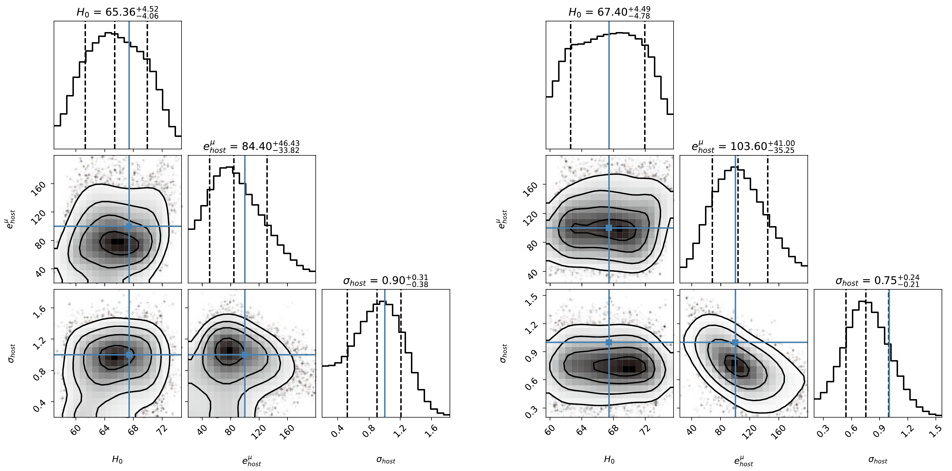

Figure 3.  (color online) Constraints on the three free parameters ($ H_0 $, $ e^\mu $, $ \sigma_{\rm{host}} $) using 100 mock FRBs with quasi-Gaussian (left panel) and Gaussian (right panel) distributions of $ \rm DM_{IGM} $. The blue lines represent the fiducial values. The black-dashed lines from left to right in each subfigure represents the 16%, 50% and 84% quantiles of the distribution, respectively. The contours from the inner to outer represent $ 1\sigma $, $ 2\sigma $, and $ 3\sigma $ confidence regions, respectively. For simplicity, units are omitted in this figure.

For comparison, the contour plots corresponding to a Gaussian distribution of $ \rm DM_{IGM} $ constrained from $ N= $ 100 mock FRBs are also presented in the right panel of Fig. 3. Note that the quasi-Gaussian distribution of $ \rm DM_{IGM} $ may influence the results for $ e^{\mu} $ and $ \sigma_{\rm{host}} $. However, concerning the Hubble constant, the quasi-Gaussian distribution of $ \rm DM_{IGM} $ does not affect its reliability, yielding consistent results. We also compared with $ N=500 $ mock FRBs; the results are presented in Fig. 4. For the Gaussian distribution of $ \rm DM_{IGM} $, the three parameters are well-constrained and can recover the fiducial values. In the case of the quasi-Gaussian distribution, the parameter $ e^{\mu} $ is not well-constrained, as mentioned before, owing to the influence of the $ \rm DM_{IGM} $ distribution. The Hubble constant $ H_0 $ can still be constrained, and the fiducial value is recovered within $ 1\sigma $ uncertainty, albeit with a relatively small value. These results indicate that further enlarging the FRB sample size does not significantly improve the precision of the constraint on $ H_0 $, primarily owing to the uncertainty associated with $ f_{\rm{IGM}} $.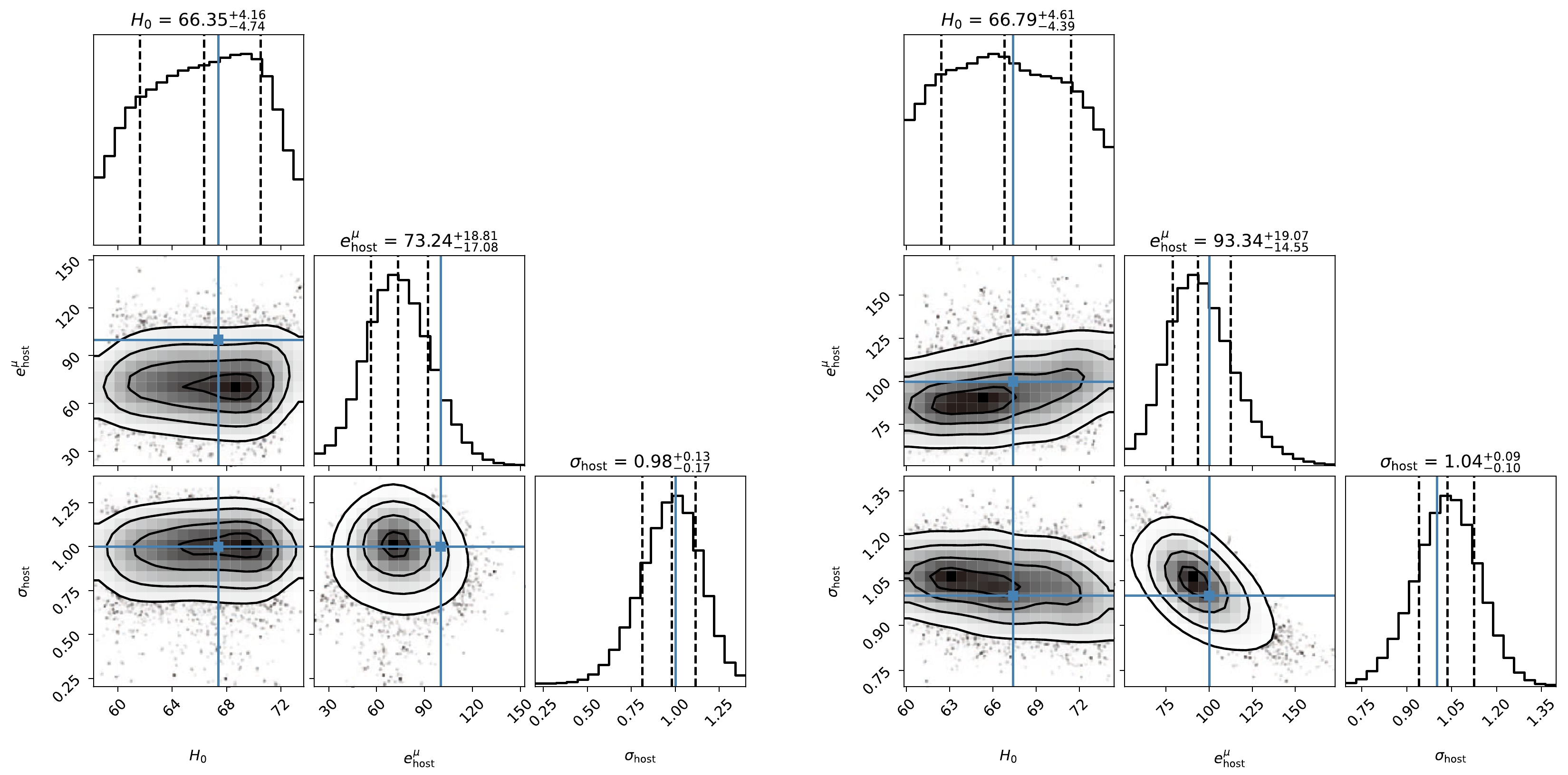

Figure 4.  (color online) Constraints on the three free parameters ($ H_0 $, $ e^\mu $, $ \sigma_{\rm{host}} $) using 500 mock FRBs with quasi-Gaussian (left panel) and Gaussian (right panel) distributions of $ \rm DM_{IGM} $. The blue lines represent the fiducial values. The black-dashed lines from left to right in each subfigure represents the 16%, 50%, and 84% quantiles of the distribution, respectively. The contours from the inner to outer represent $ 1\sigma $, $ 2\sigma $, and $ 3\sigma $ confidence regions, respectively. For simplicity, units are omitted in this figure.

To mitigate simulation fluctuations, we repeated the simulation 100 times. Specifically, we randomly generated 100 FRB samples, with each sample containing 100 mock FRBs. The 100 mock samples were then used to constrain the three free parameters ($ H_0 $, $ e^\mu $, $ \sigma_{\rm{host}} $) using the method described above, resulting in 100 sets of best-fitting parameters. The distributions of the best-fitting parameter $ H_0 $ in the 100 simulations are shown in the left panel of Fig. 5. The fiducial values are also shown as red-solid lines. Note that the Hubble constant can be tightly constrained in all cases. For comparison, we also present the results with a Gaussian distribution of $ \rm DM_{IGM} $ in the right panel of Fig. 5. It is evident that with the quasi-Gaussian distribution of $ \rm DM_{IGM} $, the best-fitting value of $ H_0 $ is systematically lower than the fiducial value, although it is still consistent with the fiducial value within $ 1\sigma $ uncertainty. On the contrary, if $ \rm DM_{IGM} $ is modeled with a Gaussian distribution, the best-fitting value of $ H_0 $ properly recovers the fiducial value. This implies that the choice of the distribution of $ \rm DM_{IGM} $ may cause bias on the estimation of the Hubble constant.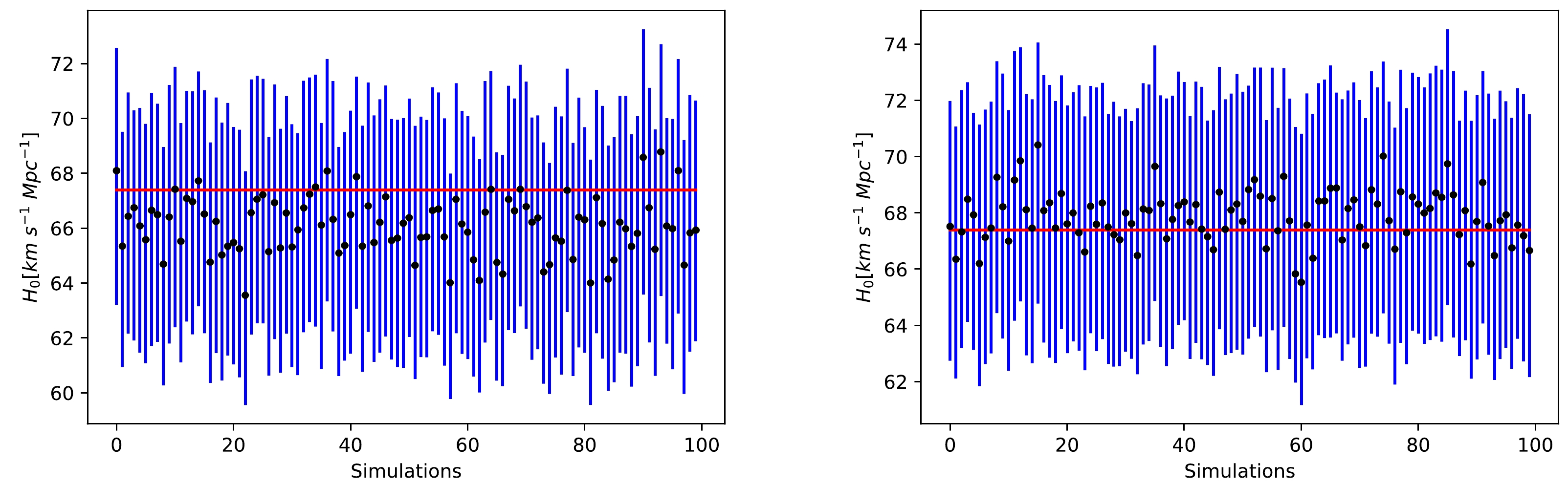

Figure 5.  (color online) Distribution of the best-fitting value for the Hubble constant shown for quasi-Gaussian (left panel) and Gaussian (right panel) distributions of $ \rm DM_{IGM} $ in 100 simulations, with $ N=100 $ FRBs in each simulation. The black dots and blue lines represent the median values of the Hubble constant and their corresponding 1σ uncertainties, respectively. The red lines represent the fiducial values.

In this study, we employed the Bayesian inference method to constrain the Hubble constant $ H_0 $, together with three FRB-related parameters ($ e^\mu $, $ \sigma_{\rm{host}} $, F) using 35 well-localized FRBs. We found that 35 FRBs could not tightly constrain four parameters simultaneously. Specifically, although the Hubble constant could be constrained, the best-fitting value $H_0=49.34^{+4.39}_{-3.83}\; {\rm{km\; s^{-1}}\; Mpc^{-1}}$ is significantly lower than that value measured by CMB. Additionally, the FRB-related parameter F was found to be much larger than expected. Subsequently, we addressed this discrepancy by fixing the parameter $ F=0.2 $ according to other observations. The three-parameter fit yielded $ H_0=60.99^{+4.57}_{-4.90}\ {\rm{km\ s^{-1}}\ Mpc^{-1}} $, a value that is still smaller than the results from CMB measurements. The relatively small median value of the Hubble constant may be attributed to the limited size of the FRB sample or the correlation between $ H_0 $ and FRB-related parameters.

Considering the anticipated growth in the number of well-located FRBs in the future, we conducted Monte Carlo simulations to assess the efficiency of the proposed method. We found that for 100 mock FRBs, $ H_0 $ was effectively constrained; however, the best-fitting value of $ H_0 $ is still lower than the fiducial value. This situation persists even if the number of FRBs is increased to 500, and the precision of the results did not significantly improve owing to the uncertainty of $ f_{\rm{IGM}} $. Further simulations revealed a systematic bias in the estimation of the Hubble constant using FRBs, although the best-fitting value of $ H_0 $ is consistent with the fiducial value within $ 1\sigma $ uncertainty. This is mainly due to the quasi-Gaussian distribution of $ \rm DM_{IGM} $, which is correlated with the Hubble constant. The bias in $ \rm DM_{IGM} $ causes a biased estimation of $ H_0 $.

The quasi-Gaussian distribution of $ \rm DM_{IGM} $ accounts for the large skew resulting from a few large-scale structures in the universe. However, the non-Gaussianity may impact the fitting results of cosmological parameters, especially the Hubble constant. To prove our hypothesis, we simulated a set of FRB samples whose $ \rm DM_{IGM} $ values were drawn from a Gaussian distribution. We then used a mock sample to constrain the Hubble constant, and compared the results with the quasi-Gaussian case, as shown in Fig. 5. We found that in the Gaussian case, the best-fitting value of $ H_0 $ correctly recovers the fiducial value. However, in the quasi-Gaussian case, the estimation of $ H_0 $ is significantly systematically biased toward a lower value than the fiducial value. Recognizing and addressing this bias is crucial for refining the fitting results of the Hubble constant.

Recently, Wu et al. [26] also used well-localized FRBs to constrain $ H_0 $ employing a quasi-Gaussian distribution of $ \rm DM_{IGM} $. They obtained values of $H_0=68.81^{+4.99}_{-4.33} {\rm{km\; s^{-1}}\; Mpc^{-1}}$ for a fixed value of $ f_{\rm{IGM}}=0.83 $, and $H_0= 69.31^{+6.21}_{-6.63}\; {\rm{km\; s^{-1}}\; Mpc^{-1}}$ if $ f_{\rm{IGM}} $ follows a uniform distribution $ U(0.747,0.913) $. The median values of both results are relatively higher than ours. The reasons for this difference are diverse. First, the FRB sample employed in the present study was much larger than theirs. Second, for other cosmological parameters, such as $ \Omega_bh^2 $ and $ \Omega_m $, Wu et al. [26] treated them as free parameters but with a uniform prior limited to a very small range. This is approximately equivalent to fixing these two parameters, as done in our study. Third, for the $ \rm DM_{halo} $ term, we set it as a constant, while Wu et al. [26] described it using a Gaussian distribution. Finally, the main difference is the treatment of FRB-related parameters. For parameters (A, $ C_0 $, $ e^{\mu},\ \sigma_{\rm{host}} $, F) in the probability functions of $ \rm DM_{host} $ and $ \rm DM_{IGM} $, Wu et al. [26] set their values according to the results of the state-of-the-art IllustrisTNG simulation. This approach may introduce a loop problem due to the fiducial parameter settings in the IllustrisTNG simulation. The method employed by Wu et al. [26] is equivalent to fixing the FRB-related parameters in the MCMC analysis. In the present study, the FRB-related parameters were set free. Given that the FRB-related parameters are correlated with the Hubble constant, the estimation on $ H_0 $ in this study is biased and has large uncertainty.