Quasi-normal modes, emission rate, and shadow of charged AdS black holes with perfect fluid dark matter

Hao Chen; Shi-Hai Dong; Sepehr Hassanabadi; Narges Heidari; Hassan Hassanabadi

doi:10.1088/1674-1137/ad4af4

Chinese Physics C> 2024, Vol. 48> Issue(8) : 085105 DOI: 10.1088/1674-1137/ad4af4

Quasi-normal modes, emission rate, and shadow of charged AdS black holes with perfect fluid dark matter

Hao Chen ^{1,,

,} ,
Shi-Hai Dong ^{2,3,
,} ,
Sepehr Hassanabadi ^4, ,
Narges Heidari ^5, ,
Hassan Hassanabadi ^5,6,

1.
School of Physics and Electronic Science, Zunyi Normal University, Zunyi 563006, China
2.
Research Center for Quantum Physics, Huzhou University, Huzhou 313000, China
3.
Centro de Investigación en Computación, Instituto Politécnico Nacional, UPALM, Mexico City 07700, Mexico
4.
Department of Physics, University of Tehran, North Karegar Avenue, Tehran 14395-547, Iran
5.
Faculty of Physics, Shahrood University of Technology, Shahrood, Iran
6.
Department of Physics, University of Hradec Králové, Rokitanského 62, 500 03 Hradec Králové, Czechia

Abstract
HTML
Reference
Related

PDF

Abstract：
In this study, we comprehensively investigated charged AdS black holes surrounded by a distinct form of dark matter. In particular, we focused on key elements including the Hawking temperature, quasi-normal modes (QNMs), emission rate, and shadow. We first calculated the Hawking temperature, thereby identifying critical values such as the critical radius and maximum temperature of the black hole, essential for determining its phase transition. Further analysis focused on the QNMs of charged AdS black holes immersed in perfect fluid dark matter (PFDM) within the massless scalar field paradigm. Employing the Wentzel-Kramers-Brillouin (WKB) method, we accurately derived the frequencies of these QNMs. Additionally, we conducted a meticulous assessment of how the intensity of the PFDM parameter α influences the partial absorption cross sections of the black hole, along with a detailed study of the frequency variation of the energy emission rate. The pivotal role of geodesics in understanding astrophysical black hole characteristics is highlighted. Specifically, we examined the influence of the dark matter parameter on photon evolution by computing the shadow radius of the black hole. Our findings distinctly demonstrate the significant impact of the PFDM parameter α on the boundaries of this shadow, providing crucial insights into its features and interactions. We also provide profound insights into the intricate dynamics between a charged AdS black hole, novel dark matter, and various physical phenomena, elucidating their interplay and contributing valuable knowledge to the understanding of these cosmic entities.
- black hole ,
- dark matter ,
- quasi-normal modes ,
- greybody factor ,
- shadow radius

I. INTRODUCTION

I. INTRODUCTION
II. THERMODYNAMICS OF A CHARGED ADS BLACK HOLE WITH PFDM
III. QNMs AND EMISSION RATE OF THE CHARGED AdS BLACK HOLE WITH PFDM
IV. SHADOW OF A CHARGED ADS BLACK HOLE WITH PFDM
V. CONCLUSION
ACKNOWLEDGMENTS

The General Theory of Relativity, introduced in 1915, is the foremost comprehensive explanation of gravitational phenomena. Notably, Einstein's field equations, formulated within this theory, predicted the existence of one of the most enigmatic entities in the cosmos: the black hole. Originating from the collapse and subsequent extinguishment of massive stars, black holes manifest as exceedingly compact regions with gravitational forces so intense that even light cannot escape their grasp. The oscillations of black holes have been observed to emit gravitational radiation, carrying pivotal information about their internal characteristics [1, 2]. Observations of supermassive black holes, such as those in M87* [3−5] and Sagittarius A* [6, 7], provide compelling evidence supporting the existence of these enigmatic entities within our universe. The formation of the shadow of a black hole primarily arises from the gravitational deflection of light [8, 9]. Accurate measurement and analysis of this shadow offer valuable insights into the gravitational field surrounding the black hole [10−14].

The study of black hole oscillations when subjected to external perturbations is central in the analysis of the stability of the spacetime of black holes. This study primarily examined the evolution of the background field or black hole mergers. When an external field is present, it triggers the generation of QNMs in scalar [15], electromagnetic [16], and gravitational fields [17] surrounding the black hole. These QNMs, characterized by complex frequencies, dominate the gravitational waves emitted during perturbation processes. The real component of the frequency represents the oscillation frequency exhibited by the black hole, while the imaginary part denotes its decay rate. The study of these QNMs offers valuable insights into properties within the event horizon radius of a black hole [18]. Gravitational waves are emitted during the merger phase when black holes collide. The first detection of these waves from black hole mergers was announced by LIGO/VIRGO in 2016 [19]. The phenomenon known as ringdown in gravitational wave signals is intriguing, providing essential insights into the complexities of black hole physics. Ring decay refers to the rapid attenuation of oscillations observed towards the end of the waveform, representing QNMs exhibited by remnants of black holes during this phase. These QNMs can be conceptualized as characteristic vibrations or resonances arising when perturbations disrupt the event horizon of a black hole. QNMs in black holes have attracted significant attention from the academia. In Ref. [20], the authors explored the pseudo-spectra of non-horizon exotic compact objects (ECOs) with reflective surfaces situated near Schwarzschild radii. Their findings revealed that the QNMs of ECOs are influenced by their spectral instability, offering valuable insights into the dynamic behavior of peculiar entities surrounding black holes and the mechanism behind gravitational wave signals. Moreover, in Ref. [21], researchers discovered that, despite the distinct QNM spectra exhibited by black holes, very compact objects with rings demonstrate a similar decay phase in their rings. Therefore, precise observation of the late-time decay signal becomes crucial to eventually distinguish differences in QNM spectra. The WKB method is widely acknowledged as one of the primary mathematical tools for studying QNMs. Konoplya and Zhidenko proposed a more precise sixth-order WKB method to accurately compute the QNMs and grey factors of various black holes [22−29].

The primary objective of this study was to explore the Hawking temperature, QNMs, shadow formation, and emission rate of charged AdS black holes encompassed by perfect fluid dark matter. In the context of the standard cosmological model, astronomical observations have led to conclude that dark energy constitutes approximately 73% of the cosmos, while dark matter accounts for approximately 23%, with baryonic matter making up a mere 4% [30]. Theoretical models, such as the quintessence and quintom models, have been proposed to explain these empirical findings [31−33]. Interestingly, the quintessence model focuses on elucidating the relationship between the pressure of dark energy and its energy density. Understanding the interplay between quintessence and black holes holds significant importance in the realm of cosmology. Building upon Kiselev's groundbreaking work [34], this study further investigated the Schwarzschild black hole solution enveloped by quintessence. Extensive research has been carried out on various black holes immersed in quintessence matter [35−39]. Although real dark matter or dark energy could not satisfy the perfect fluid condition, perfect fluid is a good approximation to describe their behaviour. PFDM has attracted considerable research attention as a novel dark matter model owing to its efficacy in explaining the asymptotically flat rotation curve observed in spiral galaxies [40−42]. Despite manifesting gravitational effects across diverse systems, the true nature of PFDM remains enigmatic [43−45]. Another important difference between black holes in AdS space and flat or de Sitter space-time is that the horizon of black holes in flat or de Sitter space must have a spherical structure, while the horizon topology of black holes in AdS spacetime could be a zero or exhibits a negative constant curvature surface, except for the case with a positive constant curvature surface. These types of black holes with zero or negative constant curvature horizon have been studied in the literature [46−59].

Recently, Abbas and Ali conducted a detailed analysis on the thermodynamic properties concerning the stability of phase transitions in charged AdS black holes immersed in PFDM [60]. In this study, we aimed to provide pivotal insights into the horizon structure of charged AdS black holes hosting PFDM through a comprehensive analysis of their stability. Our investigation explored the Hawking temperature and QNMs of these black holes and evaluated the energy emission rate akin to Hawking radiation using grey-body factors. Additionally, we aimed at computing the shadow radius of the black hole to offer valuable insights for astronomical observations focused on charged AdS black holes featuring PFDM.

The structure of this paper is as follows. Section II provides a concise review of the solution representing a charged AdS black hole immersed in PFDM. This section also includes an analysis of the critical radius and maximum temperature associated with the phase transition of the black hole. In Sec. III, our focus shifts to analyzing the real and imaginary components within the spectrum of QNM frequencies pertaining to the black hole. Additionally, we examine the grey-body factor of the black hole and the energy emission rate akin to the Hawking radiation of the black hole. In Sec. IV, we elaborate on the shadow radius of the black hole. This section aims to provide insights into the observational aspects related to the shadow of the black hole. Lastly, Sec. V concludes the paper by summarizing our findings and the implications drawn from the outcomes obtained.

II. THERMODYNAMICS OF A CHARGED ADS BLACK HOLE WITH PFDM

I. INTRODUCTION
II. THERMODYNAMICS OF A CHARGED ADS BLACK HOLE WITH PFDM
III. QNMs AND EMISSION RATE OF THE CHARGED AdS BLACK HOLE WITH PFDM
IV. SHADOW OF A CHARGED ADS BLACK HOLE WITH PFDM
V. CONCLUSION
ACKNOWLEDGMENTS

The electromagnetic and PFDM fields are widely acknowledged to exhibit minimal coupling with gravity and the cosmological constant [61]. The solution for a charged AdS black hole with PFDM results in an expression for the metric as follows [60]:

$N(r) = 1 - \frac{{2m}}{r} + \frac{{{Q^2}}}{{{r^2}}} - \frac{1}{3}\Lambda {r^2} + \frac{\alpha }{r}\ln\frac{r}{|\alpha| }.$

(1)

Based on this metric, we can explore the distinct properties and traits of black holes. As the strength parameter α tends toward zero, the black hole undergoes a transition into an RN AdS black hole. This specific type of black hole retains both the charge Q and mass m, existing within an antisymmetric space. Furthermore, in a scenario where the charge Q is absent, the black hole transforms into a Schwarzschild AdS black hole.

The subsequent step entails evaluating the Hawking temperature of the black hole, a crucial parameter that determines its inherent thermodynamic properties:

$T_H= \frac{1}{4\pi} \left. {\frac{\mathrm{d}N(r)}{\mathrm{d}r}} \right|_{r = {r_{h}}}.$

(2)

We calculate the outer horizon by setting the lapse function to be zero:

$N(r_h) = 1 - \frac{{2M}}{r_h} + \frac{{{Q^2}}}{{{r_h^2}}} - \frac{1}{3}\Lambda {r_h^2} + \frac{\alpha }{r_h}\ln\frac{r_h}{|\alpha| }=0.$

(3)

According to Eq. (3), the mass can be expressed as a function of the horizon radius as

$M=\frac{1}{2}\left[\frac{r_h^3}{\bar{l}^2}+\frac{Q^2}{r_h}+\alpha \ln \left(\frac{r_h}{|\alpha|}\right)+r_h\right],$

(4)

where we use $\Lambda=-3/\bar{l}^{2}$ . Therefore, the Hawking temperature is expressed by the following equation:

$T_H=\frac{\bar{l}^{2} \left(r_{h} (\alpha +r_{h}-Q^2)\right)+3 r_{h}^4}{4 \pi \bar{l}^2 r_{h}^3}.$

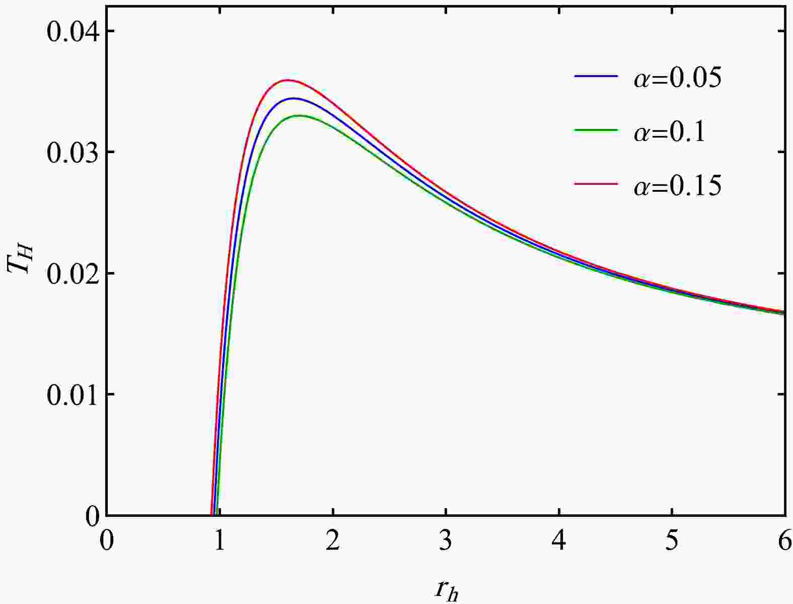
(5)

Figure 1 shows the Hawking temperature versus the horizon radius. The analysis demonstrates that the evaporation of the black hole gives rise to a residual mass that emerges in the final stage, contingent upon the α parameter. By setting Eq. (5) to zero, we can calculate this residual mass, which is listed for various α values alongside their associated radii ( $r_{\rm rem}$ ) in Table 1. Additionally, the critical radius ( $r_{\rm cr}$ ) and maximum temperature ( $T_{\rm max}$ ), indicative of the phase transition, have also been determined.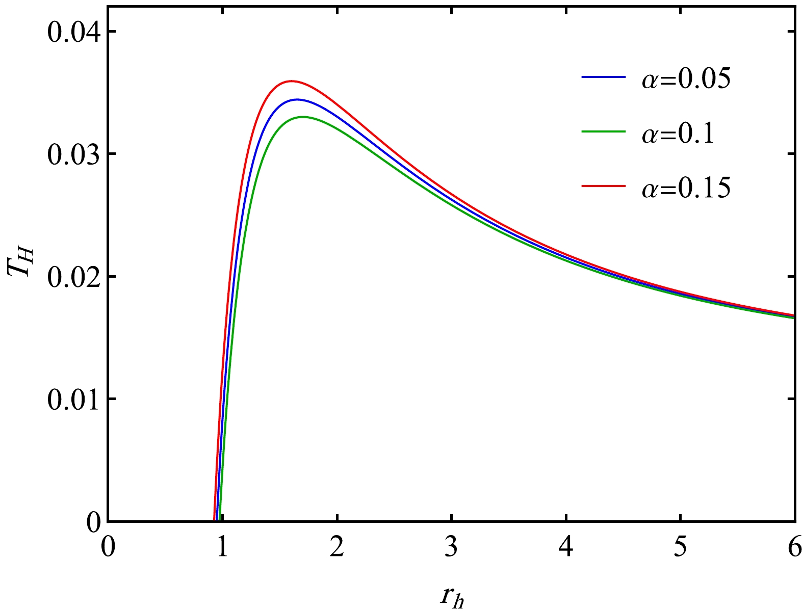

Figure 1

Figure 1. (color online) Hawking temperature for

$Q=1$ ,

$\bar{l}=20$ and various values of α.

DownLoad: Full-Size Img PowerPoint

Table 1

Table 1.

$Q=1$ ,

$\bar{l}=20$ and various values of parameter α.

α	$r_{\rm cr}$	$r_{\rm rem}$	$M_{\rm rem}$	$T_{\rm max}$
0.10	1.65092	0.948217	1.11495	0.0344216
0.15	1.60271	0.925066	1.14047	0.0359256
0.20	1.55613	0.902509	1.15687	0.0375213
0.25	1.51114	0.880543	1.16634	0.0392136
0.30	1.46771	0.859165	1.17016	0.0410079
0.35	1.42581	0.838371	1.16918	0.0429096
0.40	1.38539	0.818155	1.16401	0.0449242
0.45	1.34643	0.798512	1.1551	0.0470577
0.50	1.30887	0.779433	1.14279	0.0493158

DownLoad: CSV

Show Table

III. QNMs AND EMISSION RATE OF THE CHARGED AdS BLACK HOLE WITH PFDM

I. INTRODUCTION
II. THERMODYNAMICS OF A CHARGED ADS BLACK HOLE WITH PFDM
III. QNMs AND EMISSION RATE OF THE CHARGED AdS BLACK HOLE WITH PFDM
IV. SHADOW OF A CHARGED ADS BLACK HOLE WITH PFDM
V. CONCLUSION
ACKNOWLEDGMENTS

The perturbation caused by the scalar field interacting with the black hole is mathematically expressed through the covariant Klein-Gordon equation in curved space-time,

$\frac{1}{{\sqrt { - g} }}{\partial _\mu }(\sqrt { - g} {g^{\mu \nu }}{\partial _\nu }\Psi _{\omega lm} ) = 0,$

(6)

where we use the metric

${\rm d}{s^2} = - N(r){\rm d}{t^2} + N ^{ - 1}(r){\rm d}{t^2} + {r^2}{\rm d}{\Omega ^2},$

(7)

with $N(r)$ being determined by Eq. (1).

Next, we proceed by assuming that the wave function within this spherically symmetric system can be decomposed into the following form:

${\Psi _{\omega lm}}(\mathbf{r}, t) = \frac{{{R_{\omega l}}(r)}}{r}{Y_{lm}}(\theta , \varphi ) {{\rm e}^{- {\rm i}\omega t}},$

(8)

where $Y_{lm}(\theta, \varphi)$ represents the spherical harmonics, and ω denotes the complex QNM frequency. Upon substituting the decomposed wave function $\Psi_{\omega lm}(\mathbf{r}, t)$ into Eq. (6), we derive the radial wave function $R_{\omega l}(r)$ as follows:

$N(r)\frac{\rm d}{{{\rm d}r}}\left(N(r)\frac{{{\rm d}{R_{\omega l}}}}{{{\rm d}r}}\right)+ ({\omega ^2} - {V_{\rm eff.}}){R_{\omega l}} = 0.$

(9)

Here, $V_{\rm eff.}(r)$ , which is called the effective potential, has the following form:

$V_{\rm eff.}(r) = N(r)\frac{{l(l + 1)}}{{{r^2}}}+ \frac{{N(r)}}{r}\frac{{\mathrm{d}N}}{{\mathrm{d}r}}.$

(10)

Then, by employing a tortoise coordinate defined as ${\rm d}r^* ={\rm d}r/N(r)$ in Eq. (9), we transform the equation into a Schrödinger-like form:

$\left[\frac{{{{\rm d}^2}}}{{{\rm d}{{r^*}^2}}} + {\omega ^2} - {{V}_{\rm eff.}}\right]R_{\omega l} (r^*) = 0.$

(11)

Various approaches have been employed to explore the wave function and scattering properties [62−67]. One frequently used method for QNM analysis, initially suggested by Schutz and Will [68], is the WKB method [22, 23]. Notably, higher-order corrections for this method have been proposed by Konoplya [24, 25]. In our investigation, we aimed to assess the influence of the parameter α associated with a charged AdS black hole featuring PFDM on its QNMs. These QNMs can be computed by solving the wave equation presented in Eq. (11) using the sixth-order WKB approximation method. Within this approach, the QNMs are determined based on boundary conditions that mandate outgoing waves extending to infinity and incoming waves reaching the event horizon exclusively. The expression for the QNMs is given by

$\frac{{\rm i}(\omega^2-V_{0})}{\sqrt{-2 V^{''}_{0}}} - \sum\limits^{6}_{j=2} \Omega_{j} = n + \frac{1}{2}.$

(12)

Here, $V^{''}_{0}$ denotes the second derivative of the potential evaluated at its maximum point $r_{0}^*$ , while $\Omega_{j}$ represents correction terms dependent on the effective potential and its derivatives at this maximum. The QNMs are denoted by ω, having a form $\omega=\omega_R-{\rm i} \omega_I$ . Figures 2−5 show the real and imaginary parts of the QNMs, computed using the sixth-order WKB method, for various values of the parameter α. These figures are categorized based on the multipole number l, as shown in Figs. 2, 3, 4, and 5, corresponding to $l=0, 1, 2$ , and $3$ , respectively. The results presented in the tables indicate a trend in which both the real frequency and magnitude of the imaginary components of the QNMs increase with higher values of the α parameter. Our findings suggest that higher α values lead to higher propagating frequencies and faster damping of scalar waves.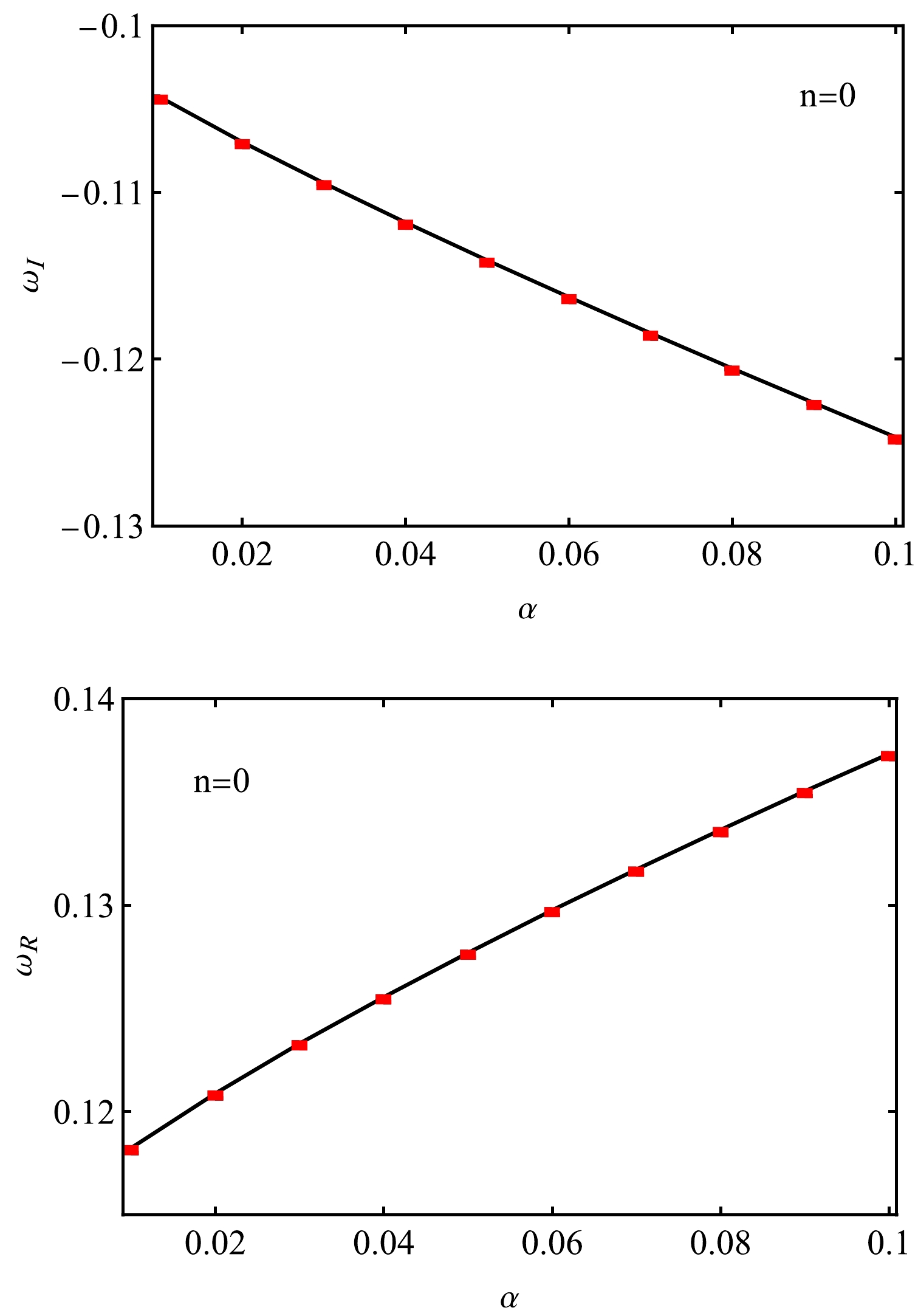

Figure 2

Figure 2. (color online) Variation of real

$\omega_R$ and imaginary

$\omega_R$ QNMs with α, using

$M = 1$ ,

$Q = 0. 2$ ,

$\bar{l} = 20$ ,

$l=0$ , and its related monopole

$n\leq l$ .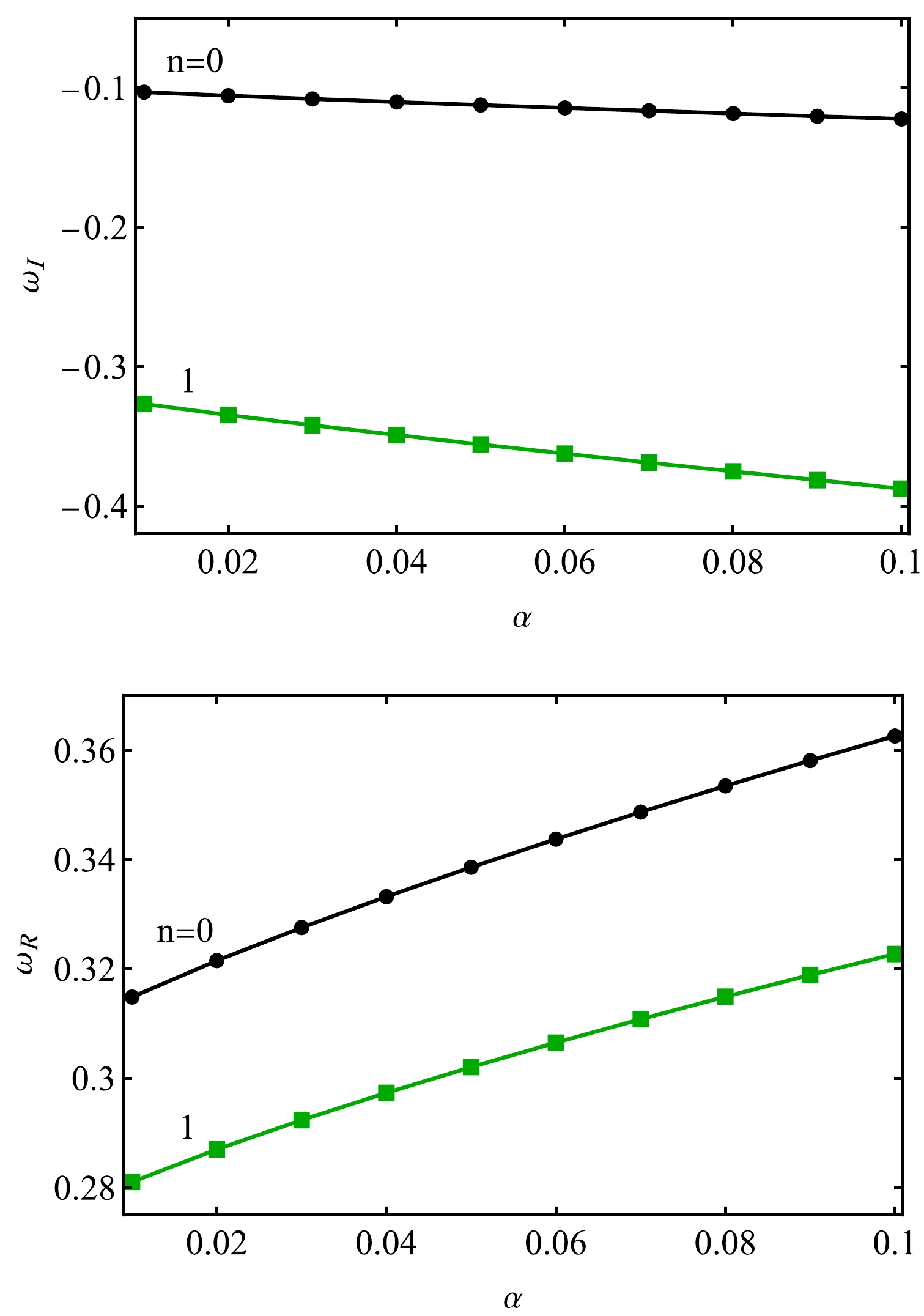

DownLoad: Full-Size Img PowerPoint

Figure 3

Figure 3. (color online) Variation of real

$\omega_R$ and imaginary

$\omega_R$ QNMs with α, using

$M = 1$ ,

$Q = 0. 2$ ,

$\bar{l} =20$ ,

$l=1$ , and its related monopole

$n\leq l$ .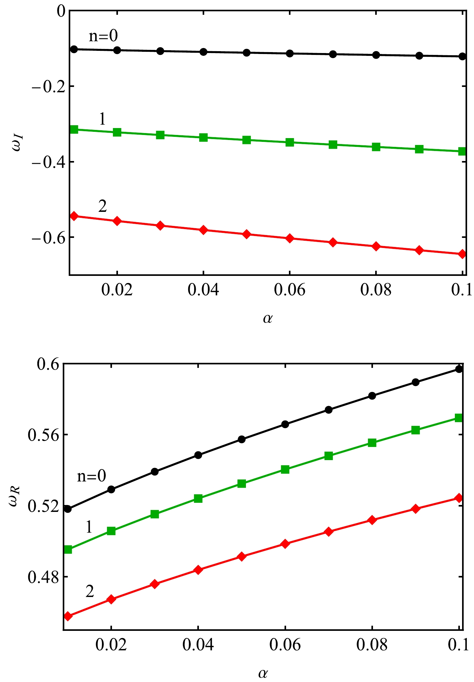

DownLoad: Full-Size Img PowerPoint

Figure 4

Figure 4. (color online) Variation of real

$\omega_R$ and imaginary

$\omega_R$ QNMs with α, using

$M = 1$ ,

$Q = 0. 2$ ,

$\bar{l} =20$ ,

$l=2$ , and its related monopole

$n\leq l$ .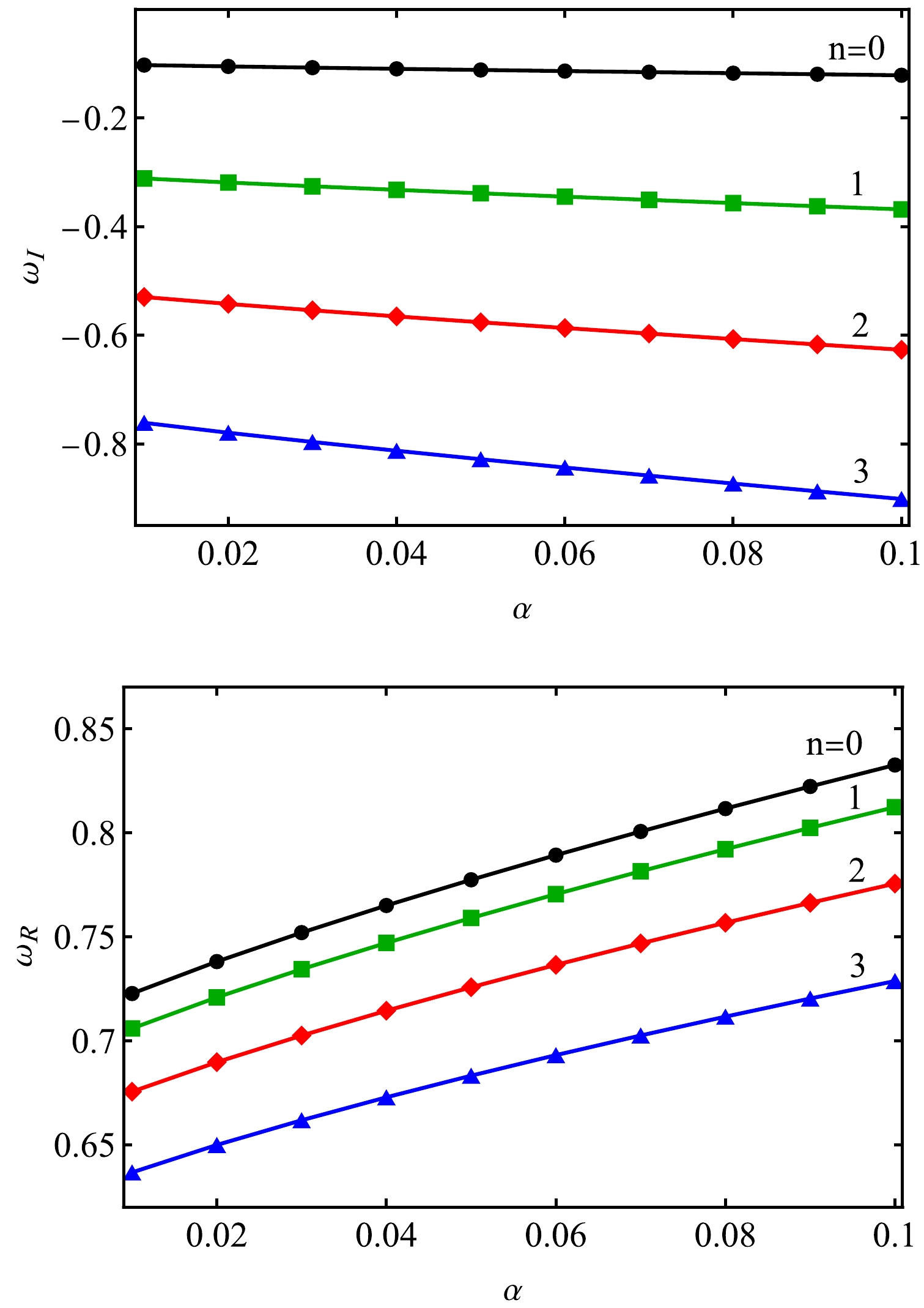

DownLoad: Full-Size Img PowerPoint

Figure 5

Figure 5. (color online) Variation of real

$\omega_R$ and imaginary

$\omega_R$ QNMs with α, using

$M = 1$ ,

$Q = 0. 2$ ,

$\bar{l} = 20$ ,

$l=3$ , and its related monopole

$n\leq l$ .

DownLoad: Full-Size Img PowerPoint

Furthermore, the WKB method has demonstrated its efficacy in analyzing wave scattering and absorption cross-sections within black hole spacetimes. The grey-body factor, a critical element in determining the tunneling probability through the potential of a black hole [69−71], relies on the probability of either incoming waves being absorbed or outgoing waves reaching infinity. This factor can be determined via the WKB method by imposing appropriate boundary conditions expected near the horizon and at infinity [27]:

$\begin{array}{*{20}{l}} R_{\omega l}= \begin{cases} {{{\rm e}^{ - {\rm i}\omega {r^*}}} + R{{\rm e}^{{\rm i}\omega {r^*}}}} \quad {\rm if}\ {r^*} \to -\infty \; (r \to {r_{h}}),\\ {T{{\rm e}^{ - {\rm i}\omega {r^*}}}} \quad \quad \quad \quad {\rm if} \ {r^*} \to +\infty \; (r \to \infty ), \end{cases} \end{array}$

(13)

The reflection coefficient is symbolized as R, while the transmission coefficient is defined as T. When employing the WKB method to investigate the influence of the PFDM parameter α on the scattering problem [24, 27, 72], it can be expressed more precisely as follows:

$|R|^{2} = \frac{1}{1+{\rm e}^{-2{\rm i}\pi \Upsilon}},$

(14)

$|T|^{2} = \frac{1}{1+{\rm e}^{+2{\rm i}\pi \Upsilon}}=1-|R|^{2},$

(15)

where $\Upsilon$ is the phase factor; $\Upsilon$ can be expressed as [73]

$\Upsilon= \frac{{\rm i}({\omega}^{2}-V_{0})}{\sqrt{-2 V''_{0}}} - \sum\limits_{j=2}^{6} \Omega_{j}(\Upsilon).$

(16)

The coefficients $\Omega_{j}(\Upsilon)$ represent functions of the effective potential, its derivatives, and the quantity $\Upsilon$ . With this information, we can calculate the grey-body factor using the following expression:

${\left| A_l \right|^2} =1-{\left| R_l \right|^2}= \frac{1}{{1 + {{\rm e}^{ + 2{\rm i}\pi {\rm \Upsilon}}}}},$

(17)

Figure 6 presents the grey-body factors of the scalar field computed using the WKB method for different values of the dark matter parameter α ( $l=1$ ). The graphical representation demonstrates that an increase in the α value results in a reduction of the grey-body factors. This decrease means that a smaller portion of the scalar field can traverse through the potential barrier. The computation of the partial absorption cross-section involves utilizing the transmission coefficient [73−75], which is defined as follows: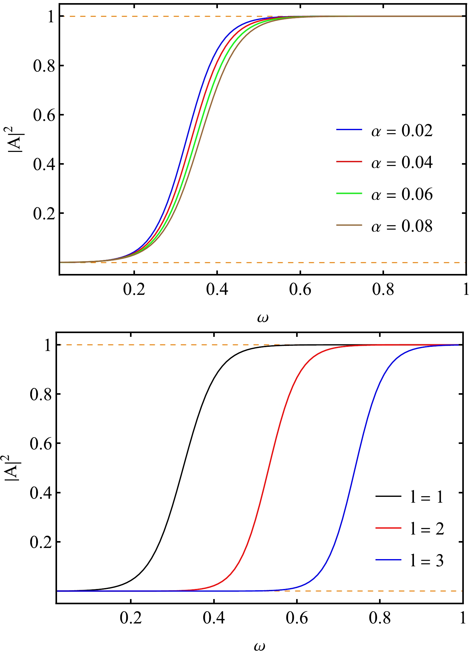

Figure 6

Figure 6. (color online) Grey-body factors of the scalar field obtained by the WKB method for

$M=1$ ,

$Q=0. 2$ , and

$\bar{l}=20$ . In the upper panel,

$l=1$ and

$\alpha=0.02, 0.04, 0.06, 0.08$ ; the lower panel shows plots for

$\alpha=0.02$ and

$l=1, 2, 3$ .

DownLoad: Full-Size Img PowerPoint

${\sigma _l} = \frac{{\pi (2l + 1)}}{{{{\omega}^2}}}{\left| {{T_l}({\omega} )} \right|^2},$

(18)

and the total absorption cross-section is derived by aggregating the partial absorption cross-sections, where l denotes the number of modes and ${\omega}$ denotes the frequency. Hence, it can be expressed as follows:

${\sigma _{abs}} = \sum\limits_l {{\sigma _l}}.$

(19)

Figure 7 depicts the partial absorption cross-sections as a function of the frequency for $l=1$ , showing variations for different values of the dark matter parameter.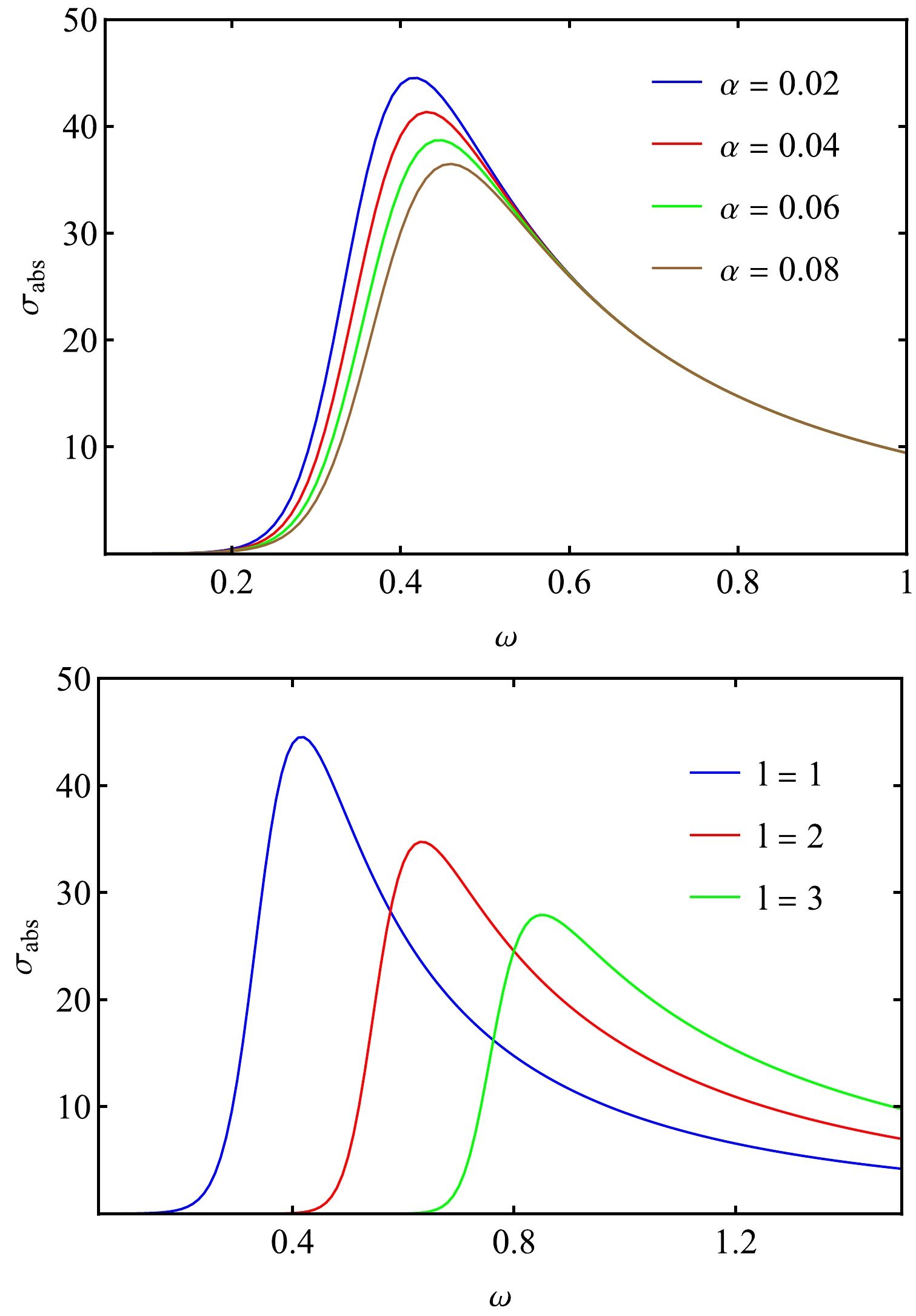

Figure 7

Figure 7. (color online) Partial absorption cross-section of the scalar field obtained from the WKB method for

$M=1$ and

$Q=0. 2$ , and

$\bar{l}=20$ . The upper panel presents plots for

$l=1$ and various values of α, whereas the lower panel shows plots for

$\alpha=0.02$ and different l values.

DownLoad: Full-Size Img PowerPoint

The plots show that higher values of the dark matter parameter correspond to lower partial absorption cross-sections. Furthermore, we analyzed the behavior of the energy emission rate with respect to the frequency.

Near black hole horizons, certain particle pairs can be generated by quantum fluctuations. Pairs with positive energy can escape from the black hole via tunneling, leading to the phenomenon known as Hawking radiation. This process is responsible for the eventual evaporation of black holes within a specific timeframe. It is important to mention that, in many scenarios, the final mass of the black hole is not considered zero owing to the existence of a residual mass in the final phase. This residual mass holds significant importance because it ensures that not all information within the black hole is lost.

According to Ref. [76], the energy emission rates are calculated as

$\frac{{{{\rm d}^2}E}}{{{\rm d}\omega {\rm d}t}} = \frac{{2{\pi ^2}\sigma {\omega ^3}}}{{{{\rm e}^{\frac{\omega }{T}}}-1}},$

(20)

where ω symbolizes the frequency of a photon, and T denotes the Hawking temperature corresponding to the outer event horizon.

Figure 8 shows the emission rate versus the frequency ω for different values of α. Note that the maximum emission rate can be determined by setting the derivative of the emission rate with respect to the frequency to zero. Additionally, according to the emission rate equation, when frequencies tend towards zero or infinity, the emission rate diminishes. Figure 8 clearly shows that, as the parameter α increases, the peak of the emission rate, representing the maximum energy emission, decreases. This escalation in α also leads to a shift of the peak of the emission rate towards lower frequencies.

Figure 8

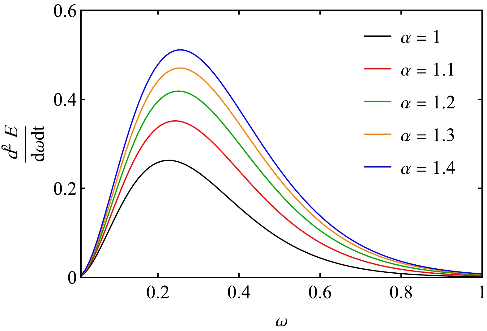
Figure 8. (color online) Emission rate for

$M=1$ ,

$Q=1$ , and

$\bar{l}=20$ for various values of α.

DownLoad: Full-Size Img PowerPoint

IV. SHADOW OF A CHARGED ADS BLACK HOLE WITH PFDM

I. INTRODUCTION
II. THERMODYNAMICS OF A CHARGED ADS BLACK HOLE WITH PFDM
III. QNMs AND EMISSION RATE OF THE CHARGED AdS BLACK HOLE WITH PFDM
IV. SHADOW OF A CHARGED ADS BLACK HOLE WITH PFDM
V. CONCLUSION
ACKNOWLEDGMENTS

Considering the initial image of a black hole revealed by the Event Horizon Telescope [3], exploring shadows and geodesics becomes profoundly significant for understanding the physical attributes of black holes [77−91]. This study aimed to investigate the equation of null geodesics and analyze the influence of the dark matter parameter on photon evolution. Assuming a spherically symmetric spacetime metric as that presented in Eq. (7), the Hamilton-Jacobi action is employed following the methodology proposed in [92]:

$\frac{{\partial S}}{{\partial \tau }} = - \frac{1}{2}{g^{\mu \nu }}\frac{{\partial S}}{{\partial {\tau ^\mu }}}\frac{{\partial S}}{{\partial {\tau ^\nu }}}.$

(21)

In this context, the Jacobi action S and the arbitrary affine parameter τ are utilized. We assume the variables to be separable, allowing us to obtain

$S = \frac{1}{2}{m^2}\tau - Et + L\phi + {S_r}(r) + {S_\theta }(\theta ).$

(22)

We express $S_r(r)$ and $S_{\theta}(\theta)$ as functions solely dependent on r and θ, respectively. Additionally, we consider a photon with zero mass ( $m=0$ ) and introduce the constants of motion—energy denoted as E and angular momentum as L—along the trajectory of the photon [92]. We can derive the null geodesic equations using Eqs. (21) and (22) as follows:

$\begin{aligned}[b] & \frac{{\mathrm{d}t}}{{\mathrm{d}\tau }} = \frac{E}{{N(r)}}, \; \; \; \frac{{\mathrm{d}r}}{{\mathrm{d}\tau }} = \frac{{\sqrt {\mathcal{R}(r)} }}{{{r^2}}},\\ & \frac{{\mathrm{d}\theta }}{{\mathrm{d}\tau }} =\pm \frac{{\sqrt {\mathcal{Q} (\theta)} }}{{{r^2}}}, \; \; \; \frac{{\mathrm{d}\varphi }}{{\mathrm{d}\tau }} = \frac{{L\, {{\csc }^2}\theta }}{{{r^2}}}, \end{aligned}$

(23)

where $\mathcal{R}(r)$ and $\mathcal{Q}(\theta)$ are defined as

$\begin{array}{*{20}{l}} \mathcal{R}(r) = {E^2}{r^4} - (\mathcal{K} + {L^2}{r^2}N(r)) \end{array}$

(24)

$\begin{array}{*{20}{l}} \mathcal{Q} (\theta ) = \mathcal{K} - {L^2}{\cot ^2}\theta, \end{array}$

(25)

and $\mathcal{K}$ is the Carter constant [93]. In this study, we only consider the equatorial plane ( $\theta=\pi/2$ ). Now, we concentrate on the radial equation:

${\left(\frac{{\mathrm{d}r}}{{\mathrm{d}\tau }}\right)^2} + {\mathcal{V}_{\rm eff.}}(r) = 0.$

(26)

Here, the effective potential is expressed as

${\mathcal{V}_{\rm eff.}}(r) = (L^2+\mathcal{K} \frac{N(r)}{{{r^2}}} - {E^2})$

(27)

and two impact parameters are introduced

$\xi = \frac{L}{E},\; \; \; \; \eta = \frac{\mathcal{K}}{{E^2}}.$

(28)

The critical radius of a photon can be determined by applying the unstable condition to the effective potential:

${\mathcal{V}_{\rm eff.}} = \frac{{\mathrm{d}{\mathcal{V}_{\rm eff.}}}}{{\mathrm{d}r}} = 0,$

(29)

which leads to

$\begin{aligned}[b] &2 - \frac{{rN'(r)}}{{N(r)}}{\uparrowvert_{r = {r_{c}}}} \equiv \\ &2- \frac{r \Big(-\dfrac{2Q^2}{r^3}+\dfrac{2m}{r^2}+\dfrac{\alpha }{r^2}-\dfrac{2 r \Lambda}{3}-\dfrac{\alpha \ln \left(\dfrac{r}{\left| \alpha \right| }\right)}{r^2}\Big)}{1 - \dfrac{{2m}}{r} + \dfrac{{{Q^2}}}{{{r^2}}} - \dfrac{1}{3}\Lambda {r^2} + \dfrac{\alpha }{r}\ln\dfrac{r}{|\alpha |}}{\uparrowvert_{r = {r_{c}}}}=0. \end{aligned}$

(30)

By applying both Eqs. (27) and (28) to the above expression, we obtain [92]

${\xi ^2} + \eta = \frac{{r_{c}^2}}{{N({r_{c}})}}.$

(31)

The shadow radius for an AdS black hole can be expressed as

$\begin{split} {R_{sh}} &= {r_{c}}\sqrt{\frac{N(r_o)}{N(r_c)}}\\ &= r_c\sqrt{\frac{1 - \dfrac{{2m}}{r_o} + \dfrac{{{Q^2}}}{{{r_o^2}}} - \dfrac{1}{3}\Lambda {r_o^2} + \dfrac{\alpha }{r_o}\ln\dfrac{r_o}{|\alpha| }}{1 - \dfrac{{2m}}{r_c} + \dfrac{{{Q^2}}}{{{r_c^2}}} - \dfrac{1}{3}\Lambda {r_c^2} + \dfrac{\alpha }{r_c}\ln\dfrac{r_c}{|\alpha| }}}, \end{split}$

(32)

where ${r_{c}}$ represents the radius of the photon sphere obtained from Eq. (30), and ${r_{o}}$ denotes the distance between the observer and black hole. By employing this formula, we can now establish constraints on the values of Λ and α based on the EHT data. Next, we examine the observational restriction on the parameters Λ and α by analyzing the data acquired from ${\rm Sgr\,A}^{*}$ in connection with the black hole shadow. According to the findings reported in Ref. [6] regarding ${\rm Sgr\,A}^{*}$ , the observational data include the distance of ${\rm Sgr\,A}^{*}$ from Earth, which is determined to be $D = 8277 \pm 33\, {\rm pc}$ , and the mass of the black hole, which is calculated to be $M_{\rm Sgr\, A^{*}}=4.3\pm 0.013 \times 10^{6}M_{\odot}$ [94, 95].

Figure 9 shows the shadow shape for different values of α. Note that, when α decreases, the radius of the shadow increases. This indicates that the shadow radius is reduced as the effect of the PFDM parameter increases.

Figure 9

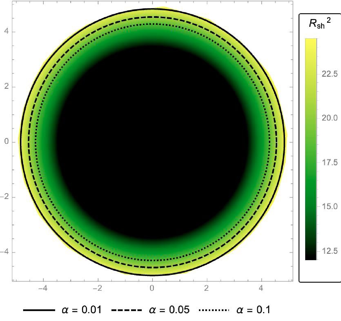
Figure 9. (color online) Shadow shape for

$M=1$ ,

$Q=1$ , and

$\bar{l}=20$ for various values of α.

DownLoad: Full-Size Img PowerPoint

Figure 10 shows the shadow shape for different values of $\bar{l}$ . Note that an increase in $\bar{l}$ results in a reduction in the radius of the shadow. However, as the value of $\bar{l}$ increases, the discrepancy in the shadow radius becomes negligible, albeit not entirely absent.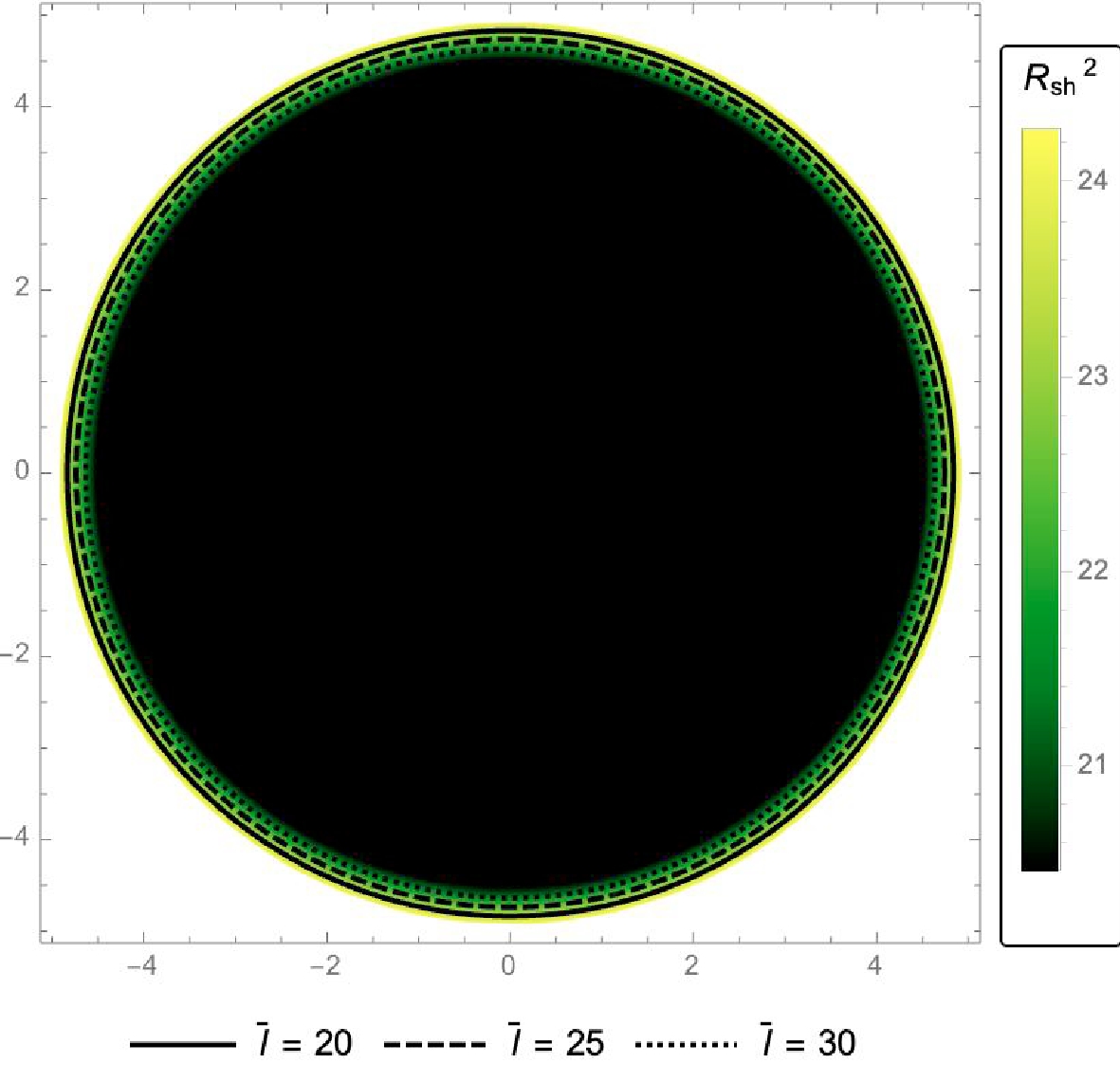

Figure 10

Figure 10. (color online) Shadow shape for

$M=1$ ,

$Q=0.1$ and

$\alpha=0.01$ for various values of

$\bar{l}$ .

DownLoad: Full-Size Img PowerPoint

The uncertainty at $1\sigma$ and $2\sigma$ levels is illustrated in Fig. 11, which depicts the variation of the shadow radius with the PFDM parameter α and cosmological constant Λ for ${\rm Sgr\,A}^{*}$ .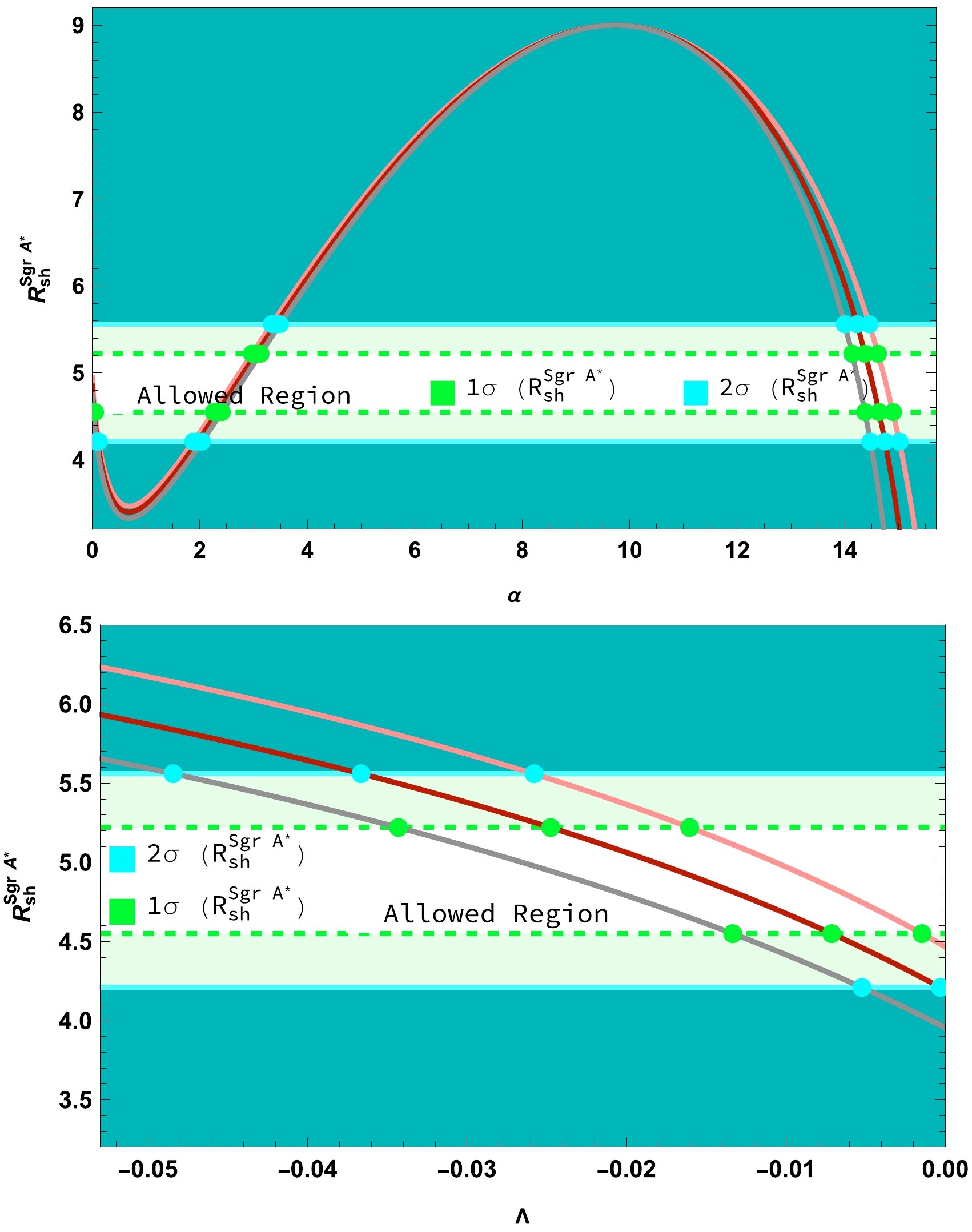

Figure 11

Figure 11. (color online) The upper panel shows the shadow radius of the black hole as a function of the parameter α for three Λ values:

$-0.007$ ,

$-0.005$ , and

$-0.003$ , represented by pink, dark red, and gray lines, respectively. In the lower panel, the shadow radius is plotted as a function of Λ, with α values of

$0.01$ ,

$0.05$ , and

$0.1$ , represented by pink, dark red, and gray lines, respectively. The black hole mass is set to

$M=1$ . The dark cyan regions indicate α and Λ values inconsistent with observations of stellar dynamics for

${\rm Sgr\,A}^{*}$ . The white and light green shaded areas correspond to the EHT horizon-scale images of Sgr A* at

$1\sigma$ and

$2\sigma$ confidence levels, respectively. In both panels, these shaded regions represent α and Λ values consistent with the averaged Keck and VLTI mass-to-distance ratio priors for

${\rm Sgr\,A}^{*}$ .

DownLoad: Full-Size Img PowerPoint

We list the upper and lower limits of the acceptable parameter values in Tables 2 and 3.

Table 2

Table 2. Acceptable values for α can be determined based on three different values of

$\Lambda = -0.007, -0.005,$ and

$-0.003$ , represented in Fig. 11 by pink, dark red, and gray lines, respectively. These values correspond to the shadow radius of the black hole that matches the EHT horizon-scale image of

${\rm Sgr\,A}^{*}$ within

$1\sigma$ and

$2\sigma$ confidence levels.

α	$1\sigma$		$2\sigma$
α	Upper	Lower	Upper	Lower
	−	$0.05$	−	$0.12$
$\Lambda = -0.007$	$2.97$	$2.26$	$3.34$	$1.88$
	$14.62$	$14.90$	$14.46$	$15.02$
	−	$0.03$	−	$0.10$
$\Lambda = -0.005$	$3.05$	$2.33$	$3.41$	$1.96$
	$14.38$	$14.64$	$14.23$	$14.75$
	−	$0.02$	−	$0.08$
$\Lambda = -0.003$	$3.13$	$2.41$	$3.49$	$2.04$
	$14.14$	$14.38$	$14.00$	$14.48$

DownLoad: CSV

Show Table

Table 3

Table 3. Acceptable values for Λ can be determined based on three different values of

$\alpha = 0.01, 0.05,$ and

$0.1$ , represented in Fig. 11 by pink, dark red, and gray lines, respectively. These values correspond to the shadow radius of the black hole that matches the EHT horizon-scale image of

${\rm Sgr\,A}^{*}$ within

$1\sigma$ and

$2\sigma$ confidence levels.

Λ	$1\sigma$		$2\sigma$
Λ	Upper	Lower	Upper	Lower
$\alpha = 0.01$	$-0.01604$	$-0.00147$	$-0.02585$	−
$\alpha = 0.05$	$-0.02476$	$-0.00713$	$-0.03665$	$-0.00031$
$\alpha = 0.1\,\,\,$	$-0.03430$	$-0.01334$	$-0.04843$	$-0.00523$

DownLoad: CSV

Show Table

We conclude that, considering various potential ranges of α and Λ at both $1\sigma$ and $2\sigma$ uncertainty levels, ${\rm Sgr\,A}^{*}$ could be a charged AdS-PFDM black hole within the current precision of astrophysical observations.

V. CONCLUSION

I. INTRODUCTION
II. THERMODYNAMICS OF A CHARGED ADS BLACK HOLE WITH PFDM
III. QNMs AND EMISSION RATE OF THE CHARGED AdS BLACK HOLE WITH PFDM
IV. SHADOW OF A CHARGED ADS BLACK HOLE WITH PFDM
V. CONCLUSION
ACKNOWLEDGMENTS

In summary, this study focused on charged AdS black holes with PFDM as the primary research subject. Our exploration involved probing the Hawking temperature of this type of black holes and analyzing the massless scalar field equation. Additionally, we employed the WKB method to determine the frequencies of the QNMs associated with the black hole while examining its partial absorption cross-section. Using the grey-body factor, we aimed at understanding how the energy emission rate varies according to frequency. Lastly, we aimed at determining the shadow radius of this particular type of black hole. Our findings encompass crucial insights into these aspects of charged AdS black holes with PFDM.

$({\rm i})$ During the final phase of black hole evaporation, a residual mass is observed, with a maximum remnant mass of $1. 17016 \;\; (Q=20, l=1, \alpha=0.3)$ . The Hawking temperature increases with the dark matter parameter α. Additionally, we provide insights into the critical radius and maximum temperature associated with the phase transition of black holes.

$({\rm ii})$ Utilizing the WKB method, we calculated the QNM frequency of the black hole. The results reveal that an increase in PFDM parameter α enhances both the real and absolute values of the imaginary part of the QNMs. Higher PFDM values lead to higher frequencies for propagating scalar waves and a faster damping rate.

$({\rm iii})$ We observed a decrease in the partial absorption cross-section as the PFDM parameter α increases. The energy emission rate diminishes as the frequency approaches zero and infinity, causing the maximum energy emission to decrease with higher parameter values. Consequently, the peak of the emission rate shifts towards lower frequencies in this scenario.

$({\rm iv})$ Figure 11 shows constraints on α and Λ based on EHT data. The upper panel displays two upper bounds and three lower bounds for both $1\sigma$ and $2\sigma$ levels. Additionally, the upper panel in Fig. 11 shows changes in the behavior of the shadow radius before and after two extremum points. Specifically, before $\alpha = 0.68$ and after $\alpha = 9.73$ , the shadow size decreases with increasing values of α; in the range $(0.68,9.73)$ , the shadow size increases with increasing values of α. In the lower panel, both upper and lower bounds are presented for the lines corresponding to $\alpha =0.05,~ 0.1$ , while for the line corresponding to $\alpha =0.01$ at the $2\sigma$ level, only one upper bound exists without a lower bound. However, at the $1\sigma$ level, both upper and lower bounds are provided. This finding may be valuable for astronomical observations of AdS black holes filled with PFDM.

ACKNOWLEDGMENTS

I. INTRODUCTION
II. THERMODYNAMICS OF A CHARGED ADS BLACK HOLE WITH PFDM
III. QNMs AND EMISSION RATE OF THE CHARGED AdS BLACK HOLE WITH PFDM
IV. SHADOW OF A CHARGED ADS BLACK HOLE WITH PFDM
V. CONCLUSION
ACKNOWLEDGMENTS

We are grateful to the referees for their insightful comments and suggestions, which have allowed us to improve this paper significantly.

References

[1]	W. Israel, Phys. Rev 164, 1776 (1967) doi: 10.1103/PhysRev.164.1776
[2]	B. Carter, Phys. Rev. Lett. 26, 331 (1971) doi: 10.1103/PhysRevLett.26.331
[3]	K. Akiyama et al. (Event Horizon Telescope Collaboration), Astrophys. J. Lett. 875, L1 (2019) doi: 10.3847/2041-8213/ab0ec7
[4]	K. Akiyama et al. (Event Horizon Telescope Collaboration), Astrophys. J. Lett. 875, L4 (2019) doi: 10.3847/2041-8213/ab0e85
[5]	K. Akiyama et al. (Event Horizon Telescope Collaboration), Astrophys. J. Lett. 875, L6 (2019) doi: 10.3847/2041-8213/ab1141
[6]	K. Akiyama et al. (Event Horizon Telescope Collaboration), Astrophys. J. Lett. 930, L12 (2022) doi: 10.3847/2041-8213/ac6674
[7]	K. Akiyama et al. (Event Horizon Telescope Collaboration), Astrophys. J. Lett. 930, L14 (2022) doi: 10.3847/2041-8213/ac6429
[8]	J. M. Bardeen, W. H. Press, and S. A. Teukolsky, Astrophys. J. 178, 347 (1972) doi: 10.1086/151796
[9]	X. J. Gao, J. M. Chen, H. Zhang et al., Phys. Lett. B 822, 136683 (2021) doi: 10.1016/j.physletb.2021.136683
[10]	Y. Mizuno, Z. Younsi, C. M. Fromm et al., Nature Astron. 2, 585 (2018) doi: 10.1038/s41550-018-0449-5
[11]	V. Perlick and O.Y. Tsupko, Phys. Rep. 947, 39 (2022) doi: 10.1016/j.physrep.2021.10.004
[12]	X. J. Gao, X. K. Yan, Y. Yin et al., Eur. Phys. J. C 83, 281 (2023) doi: 10.1140/epjc/s10052-023-11414-0
[13]	D. Anish, A. Saha, and S. Gangopadhyay, Class. Quant. Grav. 38, 065015 (2021) doi: 10.1088/1361-6382/abd95b
[14]	C. K. Qiao and M. Zhou, JCAP 12, 005 (2023) doi: 10.1088/1475-7516/2023/12/005
[15]	R. Moderski and M. Rogatko, Phys. Rev. D 64, 044024 (2001) doi: 10.1103/PhysRevD.64.044024
[16]	M. Bouhmadi-Lopez, S. Brahma, C. Y. Chen et al., arXiv: 1902.07874 [gr-qc]
[17]	C. Y. Chen and P. Chen, Phys. Rev. D 99, 104003 (2019) doi: 10.1103/PhysRevD.99.104003
[18]	C. V. Vishveshwara, Nature 227, 936 (1970) doi: 10.1038/227936a0
[19]	B. P. Abbott et al. (LIGO Scientific, Virgo Collaboration), Phys. Rev. Lett. 116, 061102 (2016) doi: 10.1103/PhysRevLett.116.061102
[20]	V. Boyanov, K. Destounis, R. Panosso Macedo et al., Phys. Rev. D 107, 064012 (2023) doi: 10.1103/PhysRevD.107.064012
[21]	V. Cardoso, E. Franzin, and P. Pani, Phys. Rev. Lett. 116, 171101 (2016) doi: 10.1103/PhysRevLett.116.171101
[22]	R. A. Konoplya and A. Zhidenko, Rev. Mod. Phys. 83, 793 (2011) doi: 10.1103/RevModPhys.83.793
[23]	R. A. Konoplya, Phys. Rev. D 66, 044009 (2002) doi: 10.1103/PhysRevD.66.044009
[24]	R. A. Konoplya, A. Zhidenko, and A F Zinhailo, Class. Quant. Grav. 36, 155002 (2019) doi: 10.1088/1361-6382/ab2e25
[25]	R. A. Konoplya, Phys. Rev. D 68, 024018 (2003) doi: 10.1103/PhysRevD.68.024018
[26]	R. A. Konoplya and A. Zinhailo, Phys. Rev. D 99, 104060 (2019) doi: 10.1103/PhysRevD.99.104060
[27]	R. A. Konoplya, Phys. Lett. B 804, 135363 (2020) doi: 10.1016/j.physletb.2020.135363
[28]	R. A. Konoplya and A. Zhidenko, JCAP 08, 008 (2023) doi: 10.1088/1475-7516/2023/08/008
[29]	R. A. Konoplya and A. Zhidenko, Phys. Rev. D 107, 044009 (2023) doi: 10.1103/PhysRevD.107.044009
[30]	D. Kastor et al., Class. Quant. Grav. 27, 235014 (2010) doi: 10.1088/0264-9381/27/23/235014
[31]	Ė. Komatsu et al. (WMAP Collaboration), Astrophys. J. Suppl. 192, 18 (2011) doi: 10.1088/0067-0049/192/2/18
[32]	R. Pantig and A. Övgün , Eur. Phys. J. C 82, 391 (2022) doi: 10.1140/epjc/s10052-022-10319-8
[33]	A. G. Riess, L. G. Strolger, J. Tonry et al., Astrophys. J. 607, 665 (2004) doi: 10.1086/383612
[34]	V. V. Kiselev, Class. Quantum Grav 20, 1187 (2003) doi: 10.1088/0264-9381/20/6/310
[35]	S. B. Chen, B. Wang, and R. Su, Phys. Rev. D 77, 124011 (2008) doi: 10.1103/PhysRevD.77.124011
[36]	G. Q. Li, Phys. Lett. B 735, 256 (2014) doi: 10.1016/j.physletb.2014.06.047
[37]	A. Younas, M. Jamil, and S. Hussain, Phys. Rev. D 92, 084042 (2015) doi: 10.1103/PhysRevD.92.084042
[38]	H. Chen, B. C. Lütfüolu, H. Hassanabadi et al., Phys. Lett. B 827, 136994 (2022) doi: 10.1016/j.physletb.2022.136994
[39]	B. Hamil and B.C. Lütfüoğlu , Nucl. Phys. B 990, 116191 (2023) doi: 10.1016/j.nuclphysb.2023.116191
[40]	G. Siddhartha, T. Matos, D. Nunez et al., arXiv: astro-ph/0003105
[41]	H. X. Zhang, Y. Chen, T. C. Ma et al., Chin. Phys. C 45, 055103 (2021) doi: 10.1088/1674-1137/abe84c
[42]	S. Qi, Q. Li, Y. Zhang et al., Mod. Phys. Lett. A 38, 2350102 (2023) doi: 10.1142/S021773232350102X
[43]	K. Saurabh and K. Jusufi, Eur. Phys. J. C 81, 490 (2021) doi: 10.1140/epjc/s10052-021-09280-9
[44]	S. Shaymatov, B. Ahmedov, and M. Jamil, Eur. Phys. J. C 81, 588 (2021) doi: 10.1140/epjc/s10052-021-09398-w
[45]	A. Das, A. R. Chowdhury, and S. Gangopadhyay, Class. Quant. Grav. 41, 015018 (2024) doi: 10.1088/1361-6382/ad0fb7
[46]	J. P.S. Lemos, Class. Quant. Grav. 12, 1081 (1995) doi: 10.1088/0264-9381/12/4/014
[47]	C.-G. Huang and C.-B. Liang, Phys. Lett. A 201, 27 (1995) doi: 10.1016/0375-9601(95)00229-V
[48]	Jose P.S. Lemos and Vilson T. Zanchin, Phys. Rev. D 54, 3840 (1996) doi: 10.1103/PhysRevD.54.3840
[49]	R.-G. Cai and Y.-Z. Zhang, Phys. Rev. D 54, 4891 (1996) doi: 10.1103/physrevd.54.4891
[50]	R.-G. Cai, J.-Y. Ji, and K.-S. Soh, Phys. Rev. D 57, 6547 (1998) doi: 10.1103/PhysRevD.57.6547
[51]	S. Aminneborg, I. Bengtsson, S. Holst et al., Class. Quant. Grav. 13, 2707 (1996) doi: 10.1088/0264-9381/13/10/010
[52]	R. B. Mann, Class. Quant. Grav., 14, L109 (1997) doi: 10.1088/0264-9381/14/5/007
[53]	L. Vanzo, Phys. Rev. D 56, 6475 (1997) doi: 10.1103/PhysRevD.56.6475
[54]	D. R. Brill, J. Louko, and P. Peldan, Phys. Rev. D 56, 3600 (1997) doi: 10.1103/PhysRevD.56.3600
[55]	D. Klemm, V. Moretti, and L. Vanzo, Phys. Rev. D 57, 6127 (1998) doi: 10.1103/PhysRevD.57.6127
[56]	R.-G. Cai and K.-S. Soh, Phys. Rev. D 59, 044013 (1999) doi: 10.1103/PhysRevD.59.044013
[57]	D. Birmingham, Class. Quant. Grav. 16, 1197 (1999) doi: 10.1088/0264-9381/16/4/009
[58]	R.-G. Cai, Phys. Rev. D 65, 084014 (2002) doi: 10.1103/PhysRevD.65.084014
[59]	M.-Y. Zhang, H. Chen, H. Hassanabadi et al., Eur. Phys. J. C 83, 773 (2023) doi: 10.1140/epjc/s10052-023-11933-w
[60]	G. Abbas and R. H. Ali, Eur. Phys. J. C 83, 407 (2023) doi: 10.1140/epjc/s10052-023-11580-1
[61]	M. H. Li and K. C. Yang, Phys. Rev. D 86, 123015 (2012) doi: 10.1103/PhysRevD.86.123015
[62]	V. Ferrari and B. Mashhoon, Phys. Rev. D 30, 295 (1984) doi: 10.1103/PhysRevD.30.295
[63]	E. W. Leaver, Proc. Roy. Soc. Lond. A 402, 285 (1985) doi: 10.1098/rspa.1985.0119
[64]	N. Heidari and H. Hassanabadi, Phys. Lett. B 839, 137814 (2023) doi: 10.1016/j.physletb.2023.137814
[65]	L. Dong, Y. Yang, A. Övgün et al., Eur. Phys. J. C 83, 565 (2023) doi: 10.1140/epjc/s10052-023-11739-w
[66]	A. Baruah, A. Övgün, and A. Deshamukhya , Ann. Phys. 455, 169393 (2023) doi: 10.1016/j.aop.2023.169393
[67]	E. Berti, V. Cardoso, and A. O. Starinets, Class. Quant. Grav. 26, 163001 (2009) doi: 10.1088/0264-9381/26/16/163001
[68]	B. F. Schutz and C. M. Will, Astrophys. J. 291, L33 (1985) doi: 10.1086/184453
[69]	i. Sakalli and S. Kanzi, Turk. J. Phys. 46, 51 (2022) doi: 10.55730/1300-0101.2691
[70]	L. C. Crispino, A. Higuchi, E. S. Oliveira et al., Phys. Rev. D 87, 104034 (2013) doi: 10.1103/PhysRevD.87.104034
[71]	V. Cardoso, M. Cavaglia, and L. Gualtieri, Phys. Rev. Lett. 96, 071301 (2006) doi: 10.1103/PhysRevLett.96.071301
[72]	J. A. V Campos, M. A. Anacleto, F.A. Brito et al., Sci. Rep. 12, 8516 (2022) doi: 10.1038/s41598-022-12343-w
[73]	S. Iyer and C. M. Will, Phys. Rev. D 35, 3621 (1987) doi: 10.1103/PhysRevD.35.3621
[74]	S. Dey and S. Chakrabarti, Eur. Phys. J. C 79, 504 (2019) doi: 10.1140/epjc/s10052-019-7004-0
[75]	H. Chen, H. Hassanabadi, B. C. Lütfüolu et al., Gen. Rel. Grav. 54, 143 (2022) doi: 10.1007/s10714-022-03037-9
[76]	S. Hawking, Commun. Math. Phys. 43, 199 (1975) doi: 10.1007/BF02345020
[77]	K. Jusufi, Phys. Rev. D 101, 124063 (2020) doi: 10.1103/PhysRevD.101.124063
[78]	H. Falcke, F. Melia, and E. Agol, Astrophys. J. 528, L13 (1999) doi: 10.1086/312423
[79]	F. Atamurotov, A. Abdujabbarov, and B. Ahmedov, Phys. Rev. D 88, 064004 (2013) doi: 10.1103/PhysRevD.88.064004
[80]	L. Amarilla and E. F. Eiroa, Phys. Rev. D 85, 064019 (2012) doi: 10.1103/PhysRevD.85.064019
[81]	P. C. Li, M. Y. Guo, and B. Chen, Phys. Rev. D 101, 084041 (2020) doi: 10.1103/PhysRevD.101.084041
[82]	I. Cimdiker, D. Demir, and A. Övgün , Phys. Dark Univ. 34, 100900 (2021) doi: 10.1016/j.dark.2021.100900
[83]	A. F. Zakharov, F. Paolis, G. Ingrosso et al., New Astron. Rev. 56, 64 (2012) doi: 10.1016/j.newar.2011.09.002
[84]	S. Vagnozzi, R. Roy, Y. D. Tsai et al., Class. Quant. Grav. 40, 16 (2023) doi: 10.1088/1361-6382/acd97b
[85]	R. Kumar and S. G. Ghosh, Astrophys. J. 892, 78 (2020) doi: 10.3847/1538-4357/ab77b0
[86]	B. Cuadros-Melgar, R. Fontana, and J. Oliveira, Phys. Lett. B 811, 135966 (2020) doi: 10.1016/j.physletb.2020.135966
[87]	R. Pantig, P. K. Yu, E. T. Rodulfo et al., Ann. Phys. 436, 168722 (2022) doi: 10.1016/j.aop.2021.168722
[88]	G. Mustafa, F. Atamurotov, I. Hussain et al., Chin. Phys. C 46, 125107 (2022) doi: 10.1088/1674-1137/ac917f
[89]	B. Hamil and B. C. Lütfüoğlu, Phys. Dark Univ. 42, 101293 (2023) doi: 10.1016/j.dark.2023.101293
[90]	Y. Yang, D. Liu, A. Övgün et al., Eur. Phys. J. C 84, 63 (2024) doi: 10.1140/epjc/s10052-024-12412-6
[91]	Y. Yang, D. Liu, A. Övgün et al., Phys. Rev. D 109, 024002 (2024) doi: 10.1103/PhysRevD.109.024002
[92]	K. Jusufi, Phys. Rev. D 101, 084055 (2020) doi: 10.1103/PhysRevD.101.084055
[93]	B. Carter, Phys. Rev. 174, 1559 (1968) doi: 10.1103/PhysRev.174.1559
[94]	E. González, K. Jusufi, G. Leon et al., Phys. Dark Univ. 42, 101304 (2023) doi: 10.1016/j.dark.2023.101304
[95]	S. Capozziello, S. Zare, D. F. Mota et al., J. Cosmol. Astropart. Phys. 05, 027 (2023) doi: 10.1088/1475-7516/2023/05/027

References

[1]	W. Israel, Phys. Rev 164, 1776 (1967) doi: 10.1103/PhysRev.164.1776
[2]	B. Carter, Phys. Rev. Lett. 26, 331 (1971) doi: 10.1103/PhysRevLett.26.331
[3]	K. Akiyama et al. (Event Horizon Telescope Collaboration), Astrophys. J. Lett. 875, L1 (2019) doi: 10.3847/2041-8213/ab0ec7
[4]	K. Akiyama et al. (Event Horizon Telescope Collaboration), Astrophys. J. Lett. 875, L4 (2019) doi: 10.3847/2041-8213/ab0e85
[5]	K. Akiyama et al. (Event Horizon Telescope Collaboration), Astrophys. J. Lett. 875, L6 (2019) doi: 10.3847/2041-8213/ab1141
[6]	K. Akiyama et al. (Event Horizon Telescope Collaboration), Astrophys. J. Lett. 930, L12 (2022) doi: 10.3847/2041-8213/ac6674
[7]	K. Akiyama et al. (Event Horizon Telescope Collaboration), Astrophys. J. Lett. 930, L14 (2022) doi: 10.3847/2041-8213/ac6429
[8]	J. M. Bardeen, W. H. Press, and S. A. Teukolsky, Astrophys. J. 178, 347 (1972) doi: 10.1086/151796
[9]	X. J. Gao, J. M. Chen, H. Zhang et al., Phys. Lett. B 822, 136683 (2021) doi: 10.1016/j.physletb.2021.136683
[10]	Y. Mizuno, Z. Younsi, C. M. Fromm et al., Nature Astron. 2, 585 (2018) doi: 10.1038/s41550-018-0449-5
[11]	V. Perlick and O.Y. Tsupko, Phys. Rep. 947, 39 (2022) doi: 10.1016/j.physrep.2021.10.004
[12]	X. J. Gao, X. K. Yan, Y. Yin et al., Eur. Phys. J. C 83, 281 (2023) doi: 10.1140/epjc/s10052-023-11414-0
[13]	D. Anish, A. Saha, and S. Gangopadhyay, Class. Quant. Grav. 38, 065015 (2021) doi: 10.1088/1361-6382/abd95b
[14]	C. K. Qiao and M. Zhou, JCAP 12, 005 (2023) doi: 10.1088/1475-7516/2023/12/005
[15]	R. Moderski and M. Rogatko, Phys. Rev. D 64, 044024 (2001) doi: 10.1103/PhysRevD.64.044024
[16]	M. Bouhmadi-Lopez, S. Brahma, C. Y. Chen et al., arXiv: 1902.07874 [gr-qc]
[17]	C. Y. Chen and P. Chen, Phys. Rev. D 99, 104003 (2019) doi: 10.1103/PhysRevD.99.104003
[18]	C. V. Vishveshwara, Nature 227, 936 (1970) doi: 10.1038/227936a0
[19]	B. P. Abbott et al. (LIGO Scientific, Virgo Collaboration), Phys. Rev. Lett. 116, 061102 (2016) doi: 10.1103/PhysRevLett.116.061102
[20]	V. Boyanov, K. Destounis, R. Panosso Macedo et al., Phys. Rev. D 107, 064012 (2023) doi: 10.1103/PhysRevD.107.064012
[21]	V. Cardoso, E. Franzin, and P. Pani, Phys. Rev. Lett. 116, 171101 (2016) doi: 10.1103/PhysRevLett.116.171101
[22]	R. A. Konoplya and A. Zhidenko, Rev. Mod. Phys. 83, 793 (2011) doi: 10.1103/RevModPhys.83.793
[23]	R. A. Konoplya, Phys. Rev. D 66, 044009 (2002) doi: 10.1103/PhysRevD.66.044009
[24]	R. A. Konoplya, A. Zhidenko, and A F Zinhailo, Class. Quant. Grav. 36, 155002 (2019) doi: 10.1088/1361-6382/ab2e25
[25]	R. A. Konoplya, Phys. Rev. D 68, 024018 (2003) doi: 10.1103/PhysRevD.68.024018
[26]	R. A. Konoplya and A. Zinhailo, Phys. Rev. D 99, 104060 (2019) doi: 10.1103/PhysRevD.99.104060
[27]	R. A. Konoplya, Phys. Lett. B 804, 135363 (2020) doi: 10.1016/j.physletb.2020.135363
[28]	R. A. Konoplya and A. Zhidenko, JCAP 08, 008 (2023) doi: 10.1088/1475-7516/2023/08/008
[29]	R. A. Konoplya and A. Zhidenko, Phys. Rev. D 107, 044009 (2023) doi: 10.1103/PhysRevD.107.044009
[30]	D. Kastor et al., Class. Quant. Grav. 27, 235014 (2010) doi: 10.1088/0264-9381/27/23/235014
[31]	Ė. Komatsu et al. (WMAP Collaboration), Astrophys. J. Suppl. 192, 18 (2011) doi: 10.1088/0067-0049/192/2/18
[32]	R. Pantig and A. Övgün , Eur. Phys. J. C 82, 391 (2022) doi: 10.1140/epjc/s10052-022-10319-8
[33]	A. G. Riess, L. G. Strolger, J. Tonry et al., Astrophys. J. 607, 665 (2004) doi: 10.1086/383612
[34]	V. V. Kiselev, Class. Quantum Grav 20, 1187 (2003) doi: 10.1088/0264-9381/20/6/310
[35]	S. B. Chen, B. Wang, and R. Su, Phys. Rev. D 77, 124011 (2008) doi: 10.1103/PhysRevD.77.124011
[36]	G. Q. Li, Phys. Lett. B 735, 256 (2014) doi: 10.1016/j.physletb.2014.06.047
[37]	A. Younas, M. Jamil, and S. Hussain, Phys. Rev. D 92, 084042 (2015) doi: 10.1103/PhysRevD.92.084042
[38]	H. Chen, B. C. Lütfüolu, H. Hassanabadi et al., Phys. Lett. B 827, 136994 (2022) doi: 10.1016/j.physletb.2022.136994
[39]	B. Hamil and B.C. Lütfüoğlu , Nucl. Phys. B 990, 116191 (2023) doi: 10.1016/j.nuclphysb.2023.116191
[40]	G. Siddhartha, T. Matos, D. Nunez et al., arXiv: astro-ph/0003105
[41]	H. X. Zhang, Y. Chen, T. C. Ma et al., Chin. Phys. C 45, 055103 (2021) doi: 10.1088/1674-1137/abe84c
[42]	S. Qi, Q. Li, Y. Zhang et al., Mod. Phys. Lett. A 38, 2350102 (2023) doi: 10.1142/S021773232350102X
[43]	K. Saurabh and K. Jusufi, Eur. Phys. J. C 81, 490 (2021) doi: 10.1140/epjc/s10052-021-09280-9
[44]	S. Shaymatov, B. Ahmedov, and M. Jamil, Eur. Phys. J. C 81, 588 (2021) doi: 10.1140/epjc/s10052-021-09398-w
[45]	A. Das, A. R. Chowdhury, and S. Gangopadhyay, Class. Quant. Grav. 41, 015018 (2024) doi: 10.1088/1361-6382/ad0fb7
[46]	J. P.S. Lemos, Class. Quant. Grav. 12, 1081 (1995) doi: 10.1088/0264-9381/12/4/014
[47]	C.-G. Huang and C.-B. Liang, Phys. Lett. A 201, 27 (1995) doi: 10.1016/0375-9601(95)00229-V
[48]	Jose P.S. Lemos and Vilson T. Zanchin, Phys. Rev. D 54, 3840 (1996) doi: 10.1103/PhysRevD.54.3840
[49]	R.-G. Cai and Y.-Z. Zhang, Phys. Rev. D 54, 4891 (1996) doi: 10.1103/physrevd.54.4891
[50]	R.-G. Cai, J.-Y. Ji, and K.-S. Soh, Phys. Rev. D 57, 6547 (1998) doi: 10.1103/PhysRevD.57.6547
[51]	S. Aminneborg, I. Bengtsson, S. Holst et al., Class. Quant. Grav. 13, 2707 (1996) doi: 10.1088/0264-9381/13/10/010
[52]	R. B. Mann, Class. Quant. Grav., 14, L109 (1997) doi: 10.1088/0264-9381/14/5/007
[53]	L. Vanzo, Phys. Rev. D 56, 6475 (1997) doi: 10.1103/PhysRevD.56.6475
[54]	D. R. Brill, J. Louko, and P. Peldan, Phys. Rev. D 56, 3600 (1997) doi: 10.1103/PhysRevD.56.3600
[55]	D. Klemm, V. Moretti, and L. Vanzo, Phys. Rev. D 57, 6127 (1998) doi: 10.1103/PhysRevD.57.6127
[56]	R.-G. Cai and K.-S. Soh, Phys. Rev. D 59, 044013 (1999) doi: 10.1103/PhysRevD.59.044013
[57]	D. Birmingham, Class. Quant. Grav. 16, 1197 (1999) doi: 10.1088/0264-9381/16/4/009
[58]	R.-G. Cai, Phys. Rev. D 65, 084014 (2002) doi: 10.1103/PhysRevD.65.084014
[59]	M.-Y. Zhang, H. Chen, H. Hassanabadi et al., Eur. Phys. J. C 83, 773 (2023) doi: 10.1140/epjc/s10052-023-11933-w
[60]	G. Abbas and R. H. Ali, Eur. Phys. J. C 83, 407 (2023) doi: 10.1140/epjc/s10052-023-11580-1
[61]	M. H. Li and K. C. Yang, Phys. Rev. D 86, 123015 (2012) doi: 10.1103/PhysRevD.86.123015
[62]	V. Ferrari and B. Mashhoon, Phys. Rev. D 30, 295 (1984) doi: 10.1103/PhysRevD.30.295
[63]	E. W. Leaver, Proc. Roy. Soc. Lond. A 402, 285 (1985) doi: 10.1098/rspa.1985.0119
[64]	N. Heidari and H. Hassanabadi, Phys. Lett. B 839, 137814 (2023) doi: 10.1016/j.physletb.2023.137814
[65]	L. Dong, Y. Yang, A. Övgün et al., Eur. Phys. J. C 83, 565 (2023) doi: 10.1140/epjc/s10052-023-11739-w
[66]	A. Baruah, A. Övgün, and A. Deshamukhya , Ann. Phys. 455, 169393 (2023) doi: 10.1016/j.aop.2023.169393
[67]	E. Berti, V. Cardoso, and A. O. Starinets, Class. Quant. Grav. 26, 163001 (2009) doi: 10.1088/0264-9381/26/16/163001
[68]	B. F. Schutz and C. M. Will, Astrophys. J. 291, L33 (1985) doi: 10.1086/184453
[69]	i. Sakalli and S. Kanzi, Turk. J. Phys. 46, 51 (2022) doi: 10.55730/1300-0101.2691
[70]	L. C. Crispino, A. Higuchi, E. S. Oliveira et al., Phys. Rev. D 87, 104034 (2013) doi: 10.1103/PhysRevD.87.104034
[71]	V. Cardoso, M. Cavaglia, and L. Gualtieri, Phys. Rev. Lett. 96, 071301 (2006) doi: 10.1103/PhysRevLett.96.071301
[72]	J. A. V Campos, M. A. Anacleto, F.A. Brito et al., Sci. Rep. 12, 8516 (2022) doi: 10.1038/s41598-022-12343-w
[73]	S. Iyer and C. M. Will, Phys. Rev. D 35, 3621 (1987) doi: 10.1103/PhysRevD.35.3621
[74]	S. Dey and S. Chakrabarti, Eur. Phys. J. C 79, 504 (2019) doi: 10.1140/epjc/s10052-019-7004-0
[75]	H. Chen, H. Hassanabadi, B. C. Lütfüolu et al., Gen. Rel. Grav. 54, 143 (2022) doi: 10.1007/s10714-022-03037-9
[76]	S. Hawking, Commun. Math. Phys. 43, 199 (1975) doi: 10.1007/BF02345020
[77]	K. Jusufi, Phys. Rev. D 101, 124063 (2020) doi: 10.1103/PhysRevD.101.124063
[78]	H. Falcke, F. Melia, and E. Agol, Astrophys. J. 528, L13 (1999) doi: 10.1086/312423
[79]	F. Atamurotov, A. Abdujabbarov, and B. Ahmedov, Phys. Rev. D 88, 064004 (2013) doi: 10.1103/PhysRevD.88.064004
[80]	L. Amarilla and E. F. Eiroa, Phys. Rev. D 85, 064019 (2012) doi: 10.1103/PhysRevD.85.064019
[81]	P. C. Li, M. Y. Guo, and B. Chen, Phys. Rev. D 101, 084041 (2020) doi: 10.1103/PhysRevD.101.084041
[82]	I. Cimdiker, D. Demir, and A. Övgün , Phys. Dark Univ. 34, 100900 (2021) doi: 10.1016/j.dark.2021.100900
[83]	A. F. Zakharov, F. Paolis, G. Ingrosso et al., New Astron. Rev. 56, 64 (2012) doi: 10.1016/j.newar.2011.09.002
[84]	S. Vagnozzi, R. Roy, Y. D. Tsai et al., Class. Quant. Grav. 40, 16 (2023) doi: 10.1088/1361-6382/acd97b
[85]	R. Kumar and S. G. Ghosh, Astrophys. J. 892, 78 (2020) doi: 10.3847/1538-4357/ab77b0
[86]	B. Cuadros-Melgar, R. Fontana, and J. Oliveira, Phys. Lett. B 811, 135966 (2020) doi: 10.1016/j.physletb.2020.135966
[87]	R. Pantig, P. K. Yu, E. T. Rodulfo et al., Ann. Phys. 436, 168722 (2022) doi: 10.1016/j.aop.2021.168722
[88]	G. Mustafa, F. Atamurotov, I. Hussain et al., Chin. Phys. C 46, 125107 (2022) doi: 10.1088/1674-1137/ac917f
[89]	B. Hamil and B. C. Lütfüoğlu, Phys. Dark Univ. 42, 101293 (2023) doi: 10.1016/j.dark.2023.101293
[90]	Y. Yang, D. Liu, A. Övgün et al., Eur. Phys. J. C 84, 63 (2024) doi: 10.1140/epjc/s10052-024-12412-6
[91]	Y. Yang, D. Liu, A. Övgün et al., Phys. Rev. D 109, 024002 (2024) doi: 10.1103/PhysRevD.109.024002
[92]	K. Jusufi, Phys. Rev. D 101, 084055 (2020) doi: 10.1103/PhysRevD.101.084055
[93]	B. Carter, Phys. Rev. 174, 1559 (1968) doi: 10.1103/PhysRev.174.1559
[94]	E. González, K. Jusufi, G. Leon et al., Phys. Dark Univ. 42, 101304 (2023) doi: 10.1016/j.dark.2023.101304
[95]	S. Capozziello, S. Zare, D. F. Mota et al., J. Cosmol. Astropart. Phys. 05, 027 (2023) doi: 10.1088/1475-7516/2023/05/027

[1]	Saira Yasmin , Khadije Jafarzade , Mubasher Jamil . Shadow cast by the Kerr MOG black hole under the influence of plasma and constraints from EHT observations. Chinese Physics C, 2025, 49(6): 065107. doi: 10.1088/1674-1137/adb9c5
[2]	Ming Zhang , Rui-Hong Yue , De-Cheng Zou . Quasinormal modes of a black hole surrounded by a fluid of strings in Rastall gravity. Chinese Physics C, 2025, 49(2): 025104. doi: 10.1088/1674-1137/ad9453
[3]	Vitalii Vertogradov , Ali Övgün , Daniil Shatov . Formation of regular black hole from baryonic matter. Chinese Physics C, 2025, 49(11): 1-13.
[4]	Farruh Atamurotov , Mubasher Jamil , Kimet Jusufi . Quantum effects on the black hole shadow and deflection angle in the presence of plasma. Chinese Physics C, 2023, 47(3): 035106. doi: 10.1088/1674-1137/acaef7
[5]	Jiayi Liu , Songbai Chen , Jiliang Jing . Tidal effects of a dark matter halo around a galactic black hole. Chinese Physics C, 2022, 46(10): 105104. doi: 10.1088/1674-1137/ac7856
[6]	Chikun Ding , Xiongwen Chen . Slowly rotating Einstein-bumblebee black hole solution and its greybody factor in a Lorentz violation model. Chinese Physics C, 2021, 45(2): 025106. doi: 10.1088/1674-1137/abce51
[7]	Kun Wang , Fei Wang , Jingya Zhu , Quanlin Jie . The semi-constrained NMSSM in light of muon g-2, LHC, anddark matter constraints. Chinese Physics C, 2018, 42(10): 103109. doi: 10.1088/1674-1137/42/10/103109
[8]	Ali Övgün , Izzet Sakalli , Joel Saavedra . Quasinormal modes of a Schwarzschild black hole immersed in an electromagnetic universe. Chinese Physics C, 2018, 42(10): 105102. doi: 10.1088/1674-1137/42/10/105102
[9]	Andrea Addazi , Antonino Marcianò . Gravitational waves from dark first order phase transitions and dark photons. Chinese Physics C, 2018, 42(2): 023107. doi: 10.1088/1674-1137/42/2/023107
[10]	Guoli Liu , Fei Wang , Wenyu Wang , Jin-Min Yang . Explaining DAMPE results by dark matter with hierarchical lepton-specific Yukawa interactions. Chinese Physics C, 2018, 42(3): 035101. doi: 10.1088/1674-1137/42/3/035101
[11]	Andrea Addazi , Stephon Alexander , Yi-Fu Cai , Antonino Marcianó . Dark matter and baryogenesis in the Fermi-bounce curvaton mechanism. Chinese Physics C, 2018, 42(6): 065101. doi: 10.1088/1674-1137/42/6/065101
[12]	Peyman Zakeri , Mohammad Moosavi , Mohammadreza Zakeri , Yaser Ayazi . A minimal model for two-component FIMP dark matter: A basic search. Chinese Physics C, 2018, 42(7): 073101. doi: 10.1088/1674-1137/42/7/073101
[13]	Andrea Addazi , Pietro Donà , Antonino Marcianò . Dynamical interactions of dark energy and dark matter: Yang-Mills condensate and QCD axions. Chinese Physics C, 2018, 42(7): 075102. doi: 10.1088/1674-1137/42/7/075102
[14]	Liuyuan Shen , Yicen Mou , Yunlong Zheng , Mingzhe Li . Direct couplings of mimetic dark matter and their cosmological effects. Chinese Physics C, 2018, 42(1): 015101. doi: 10.1088/1674-1137/42/1/015101
[15]	null . Acceleration of particles in Einstein-Maxwell-dilaton black holes. Chinese Physics C, 2017, 41(6): 065101. doi: 10.1088/1674-1137/41/6/065101
[16]	Shivaramakrishna Singirala . Implications of fermionic dark matter on recent neutrino oscillation data. Chinese Physics C, 2017, 41(4): 043102. doi: 10.1088/1674-1137/41/4/043102
[17]	Gu-Qiang Li . Hawking radiation and entropy of a black hole in Lovelock-Born-Infeld gravity from the quantum tunneling approach. Chinese Physics C, 2017, 41(4): 045103. doi: 10.1088/1674-1137/41/4/045103
[18]	Yi-Ming Hu , Jin Chang , Deng-Yi Chen , Jian-Hua Guo , Yun-Long Zhang , Chang-Qing Feng . Environmental test of the BGO calorimeterfor DArk Matter Particle Explorer. Chinese Physics C, 2016, 40(11): 116003. doi: 10.1088/1674-1137/40/11/116003
[19]	S. A. Alavi , F. S. Kazemian . Photonic dark matter portal and quantum physics. Chinese Physics C, 2016, 40(2): 025101. doi: 10.1088/1674-1137/40/2/025101
[20]	HAN Yi-Wen , BAO Zhi-Qing , HONG Yun . Unruh-Verlinde temperature and energy of (2+1)-dimensional matter coupled black hole via entropic force. Chinese Physics C, 2011, 35(7): 612-615. doi: 10.1088/1674-1137/35/7/003

Access

Figures(11) / Tables(3)

Get Citation

Hao Chen, Shi-Hai Dong, Sepehr Hassanabadi, Narges Heidari and Hassan Hassanabadi. Quasi-normal modes, Emission rate and Shadow of the charged AdS black hole with perfect fluid dark matter[J]. Chinese Physics C. doi: 10.1088/1674-1137/ad4af4

RIS(for EndNote,Reference Manager,ProCite)

BibTex

Txt

Milestone

Received: 2024-03-13

Article Metric

Article Views(1610)
PDF Downloads(57)
Cited by(0)

Policy on re-use

To reuse of subscription content published by CPC, the users need to request permission from CPC, unless the content was published under an Open Access license which automatically permits that type of reuse.

通讯作者: 陈斌, bchen63@163.com

1.
沈阳化工大学材料科学与工程学院沈阳 110142

HTML

I. INTRODUCTION

The General Theory of Relativity, introduced in 1915, is the foremost comprehensive explanation of gravitational phenomena. Notably, Einstein's field equations, formulated within this theory, predicted the existence of one of the most enigmatic entities in the cosmos: the black hole. Originating from the collapse and subsequent extinguishment of massive stars, black holes manifest as exceedingly compact regions with gravitational forces so intense that even light cannot escape their grasp. The oscillations of black holes have been observed to emit gravitational radiation, carrying pivotal information about their internal characteristics [1, 2]. Observations of supermassive black holes, such as those in M87* [3−5] and Sagittarius A* [6, 7], provide compelling evidence supporting the existence of these enigmatic entities within our universe. The formation of the shadow of a black hole primarily arises from the gravitational deflection of light [8, 9]. Accurate measurement and analysis of this shadow offer valuable insights into the gravitational field surrounding the black hole [10−14].

The study of black hole oscillations when subjected to external perturbations is central in the analysis of the stability of the spacetime of black holes. This study primarily examined the evolution of the background field or black hole mergers. When an external field is present, it triggers the generation of QNMs in scalar [15], electromagnetic [16], and gravitational fields [17] surrounding the black hole. These QNMs, characterized by complex frequencies, dominate the gravitational waves emitted during perturbation processes. The real component of the frequency represents the oscillation frequency exhibited by the black hole, while the imaginary part denotes its decay rate. The study of these QNMs offers valuable insights into properties within the event horizon radius of a black hole [18]. Gravitational waves are emitted during the merger phase when black holes collide. The first detection of these waves from black hole mergers was announced by LIGO/VIRGO in 2016 [19]. The phenomenon known as ringdown in gravitational wave signals is intriguing, providing essential insights into the complexities of black hole physics. Ring decay refers to the rapid attenuation of oscillations observed towards the end of the waveform, representing QNMs exhibited by remnants of black holes during this phase. These QNMs can be conceptualized as characteristic vibrations or resonances arising when perturbations disrupt the event horizon of a black hole. QNMs in black holes have attracted significant attention from the academia. In Ref. [20], the authors explored the pseudo-spectra of non-horizon exotic compact objects (ECOs) with reflective surfaces situated near Schwarzschild radii. Their findings revealed that the QNMs of ECOs are influenced by their spectral instability, offering valuable insights into the dynamic behavior of peculiar entities surrounding black holes and the mechanism behind gravitational wave signals. Moreover, in Ref. [21], researchers discovered that, despite the distinct QNM spectra exhibited by black holes, very compact objects with rings demonstrate a similar decay phase in their rings. Therefore, precise observation of the late-time decay signal becomes crucial to eventually distinguish differences in QNM spectra. The WKB method is widely acknowledged as one of the primary mathematical tools for studying QNMs. Konoplya and Zhidenko proposed a more precise sixth-order WKB method to accurately compute the QNMs and grey factors of various black holes [22−29].

The primary objective of this study was to explore the Hawking temperature, QNMs, shadow formation, and emission rate of charged AdS black holes encompassed by perfect fluid dark matter. In the context of the standard cosmological model, astronomical observations have led to conclude that dark energy constitutes approximately 73% of the cosmos, while dark matter accounts for approximately 23%, with baryonic matter making up a mere 4% [30]. Theoretical models, such as the quintessence and quintom models, have been proposed to explain these empirical findings [31−33]. Interestingly, the quintessence model focuses on elucidating the relationship between the pressure of dark energy and its energy density. Understanding the interplay between quintessence and black holes holds significant importance in the realm of cosmology. Building upon Kiselev's groundbreaking work [34], this study further investigated the Schwarzschild black hole solution enveloped by quintessence. Extensive research has been carried out on various black holes immersed in quintessence matter [35−39]. Although real dark matter or dark energy could not satisfy the perfect fluid condition, perfect fluid is a good approximation to describe their behaviour. PFDM has attracted considerable research attention as a novel dark matter model owing to its efficacy in explaining the asymptotically flat rotation curve observed in spiral galaxies [40−42]. Despite manifesting gravitational effects across diverse systems, the true nature of PFDM remains enigmatic [43−45]. Another important difference between black holes in AdS space and flat or de Sitter space-time is that the horizon of black holes in flat or de Sitter space must have a spherical structure, while the horizon topology of black holes in AdS spacetime could be a zero or exhibits a negative constant curvature surface, except for the case with a positive constant curvature surface. These types of black holes with zero or negative constant curvature horizon have been studied in the literature [46−59].

Recently, Abbas and Ali conducted a detailed analysis on the thermodynamic properties concerning the stability of phase transitions in charged AdS black holes immersed in PFDM [60]. In this study, we aimed to provide pivotal insights into the horizon structure of charged AdS black holes hosting PFDM through a comprehensive analysis of their stability. Our investigation explored the Hawking temperature and QNMs of these black holes and evaluated the energy emission rate akin to Hawking radiation using grey-body factors. Additionally, we aimed at computing the shadow radius of the black hole to offer valuable insights for astronomical observations focused on charged AdS black holes featuring PFDM.

The structure of this paper is as follows. Section II provides a concise review of the solution representing a charged AdS black hole immersed in PFDM. This section also includes an analysis of the critical radius and maximum temperature associated with the phase transition of the black hole. In Sec. III, our focus shifts to analyzing the real and imaginary components within the spectrum of QNM frequencies pertaining to the black hole. Additionally, we examine the grey-body factor of the black hole and the energy emission rate akin to the Hawking radiation of the black hole. In Sec. IV, we elaborate on the shadow radius of the black hole. This section aims to provide insights into the observational aspects related to the shadow of the black hole. Lastly, Sec. V concludes the paper by summarizing our findings and the implications drawn from the outcomes obtained.

II. THERMODYNAMICS OF A CHARGED ADS BLACK HOLE WITH PFDM

III. QNMs AND EMISSION RATE OF THE CHARGED AdS BLACK HOLE WITH PFDM

IV. SHADOW OF A CHARGED ADS BLACK HOLE WITH PFDM

V. CONCLUSION

In summary, this study focused on charged AdS black holes with PFDM as the primary research subject. Our exploration involved probing the Hawking temperature of this type of black holes and analyzing the massless scalar field equation. Additionally, we employed the WKB method to determine the frequencies of the QNMs associated with the black hole while examining its partial absorption cross-section. Using the grey-body factor, we aimed at understanding how the energy emission rate varies according to frequency. Lastly, we aimed at determining the shadow radius of this particular type of black hole. Our findings encompass crucial insights into these aspects of charged AdS black holes with PFDM.

$({\rm i})$ During the final phase of black hole evaporation, a residual mass is observed, with a maximum remnant mass of $1. 17016 \;\; (Q=20, l=1, \alpha=0.3)$ . The Hawking temperature increases with the dark matter parameter α. Additionally, we provide insights into the critical radius and maximum temperature associated with the phase transition of black holes.

$({\rm ii})$ Utilizing the WKB method, we calculated the QNM frequency of the black hole. The results reveal that an increase in PFDM parameter α enhances both the real and absolute values of the imaginary part of the QNMs. Higher PFDM values lead to higher frequencies for propagating scalar waves and a faster damping rate.

$({\rm iii})$ We observed a decrease in the partial absorption cross-section as the PFDM parameter α increases. The energy emission rate diminishes as the frequency approaches zero and infinity, causing the maximum energy emission to decrease with higher parameter values. Consequently, the peak of the emission rate shifts towards lower frequencies in this scenario.

$({\rm iv})$ Figure 11 shows constraints on α and Λ based on EHT data. The upper panel displays two upper bounds and three lower bounds for both $1\sigma$ and $2\sigma$ levels. Additionally, the upper panel in Fig. 11 shows changes in the behavior of the shadow radius before and after two extremum points. Specifically, before $\alpha = 0.68$ and after $\alpha = 9.73$ , the shadow size decreases with increasing values of α; in the range $(0.68,9.73)$ , the shadow size increases with increasing values of α. In the lower panel, both upper and lower bounds are presented for the lines corresponding to $\alpha =0.05,~ 0.1$ , while for the line corresponding to $\alpha =0.01$ at the $2\sigma$ level, only one upper bound exists without a lower bound. However, at the $1\sigma$ level, both upper and lower bounds are provided. This finding may be valuable for astronomical observations of AdS black holes filled with PFDM.

ACKNOWLEDGMENTS

We are grateful to the referees for their insightful comments and suggestions, which have allowed us to improve this paper significantly.

Reference (95)

Quasi-normal modes, emission rate, and shadow of charged AdS black holes with perfect fluid dark matter

Abstract：

I. INTRODUCTION

I. INTRODUCTION
II. THERMODYNAMICS OF A CHARGED ADS BLACK HOLE WITH PFDM
III. QNMs AND EMISSION RATE OF THE CHARGED AdS BLACK HOLE WITH PFDM
IV. SHADOW OF A CHARGED ADS BLACK HOLE WITH PFDM
V. CONCLUSION
ACKNOWLEDGMENTS

II. THERMODYNAMICS OF A CHARGED ADS BLACK HOLE WITH PFDM

I. INTRODUCTION
II. THERMODYNAMICS OF A CHARGED ADS BLACK HOLE WITH PFDM
III. QNMs AND EMISSION RATE OF THE CHARGED AdS BLACK HOLE WITH PFDM
IV. SHADOW OF A CHARGED ADS BLACK HOLE WITH PFDM
V. CONCLUSION
ACKNOWLEDGMENTS

Figure 1

Table 1

III. QNMs AND EMISSION RATE OF THE CHARGED AdS BLACK HOLE WITH PFDM

I. INTRODUCTION
II. THERMODYNAMICS OF A CHARGED ADS BLACK HOLE WITH PFDM
III. QNMs AND EMISSION RATE OF THE CHARGED AdS BLACK HOLE WITH PFDM
IV. SHADOW OF A CHARGED ADS BLACK HOLE WITH PFDM
V. CONCLUSION
ACKNOWLEDGMENTS

Figure 2

Figure 3

Figure 4

Figure 5

Figure 6

Figure 7

Figure 8

IV. SHADOW OF A CHARGED ADS BLACK HOLE WITH PFDM

I. INTRODUCTION
II. THERMODYNAMICS OF A CHARGED ADS BLACK HOLE WITH PFDM
III. QNMs AND EMISSION RATE OF THE CHARGED AdS BLACK HOLE WITH PFDM
IV. SHADOW OF A CHARGED ADS BLACK HOLE WITH PFDM
V. CONCLUSION
ACKNOWLEDGMENTS

Figure 9

Figure 10

Figure 11

Table 2

Table 3

V. CONCLUSION

I. INTRODUCTION
II. THERMODYNAMICS OF A CHARGED ADS BLACK HOLE WITH PFDM
III. QNMs AND EMISSION RATE OF THE CHARGED AdS BLACK HOLE WITH PFDM
IV. SHADOW OF A CHARGED ADS BLACK HOLE WITH PFDM
V. CONCLUSION
ACKNOWLEDGMENTS

ACKNOWLEDGMENTS

I. INTRODUCTION
II. THERMODYNAMICS OF A CHARGED ADS BLACK HOLE WITH PFDM
III. QNMs AND EMISSION RATE OF THE CHARGED AdS BLACK HOLE WITH PFDM
IV. SHADOW OF A CHARGED ADS BLACK HOLE WITH PFDM
V. CONCLUSION
ACKNOWLEDGMENTS

References

References

Access

Article Metrics

Metrics

通讯作者: 陈斌, bchen63@163.com

Email This Article