


 Abstract
 HTML
HTML Reference
 Related
 PDF
PDF


-
The top quark was discovered in 1995 by a set of D0 and CDF experiments conducted at the Fermi National Accelerator Laboratory (Fermilab), located in the United States [1, 2]. This discovery was important for the validation of the Standard Model (SM) and the study of particle physics. The study of the nature and behavior of the top quark helps us understand physical processes such as the origin of the mass of elementary particles, and weak and strong interactions. The existence and properties of the top quark have been experimentally verified several times, including the D0 and CDF experiments at Fermilab, and the ATLAS [3] and CMS [4] experiments at the Large Hadron Collider (LHC) in Geneva, Switzerland. These experiments investigate aspects of the nature, decay modes, and interactions of the top quark through high-energy collisions and particle detection techniques. The next generation of LHC will produce top quarks in large quantities. At the upgraded Fermilab, an integrated luminosity of 10 fb–1 will produce approximately
$ 8\times{10^4} $ top quarks, while at the same luminosity, the LHC will produce approximately 100 times as many [5−7].Top quark decays with flavor violation refer to the decay processes of the top quark that violate the flavor conservation, specifically the violation of the lepton or quark flavor. While the SM predicts that the top quark predominantly decays into a W boson and a bottom quark, extensions beyond the SM allow for additional decay modes that involve different quarks or leptons [8, 9]. It is worth noting that specific details about the nature and extent of flavor violation during top quark decays require more in-depth analysis. The study of heavy particle decays via flavor-changing neutral-currents (FCNC) has played an important role in testing the SM and exploring new physics beyond the SM [10−12]. In the SM, branching ratios of the FCNC of the top quarks,
$ t\rightarrow c\gamma $ ,$ t\rightarrow cg $ ,$ t\rightarrow cZ $ , and$ t\rightarrow ch $ , are highly suppressed and beyond the detection capabilities of the LHC in the near future [13−15]. However, exotic mechanisms from new physics can greatly increase these branching ratios [16], which may be detected in the future. The SM predictions [14] and latest upper bounds on the branching ratios of$ t\rightarrow c\gamma $ ,$ t\rightarrow cg $ ,$ t\rightarrow cZ $ , and$ t\rightarrow ch $ at 95% confidence level (C.L.) [17] are listed in Table 1. Note that the current experimental bounds are much higher than the SM predictions.Decay $ Br(t\rightarrow c\gamma) $ 

$ Br(t\rightarrow cg) $ 

$ Br(t\rightarrow cZ) $ 

$ Br(t\rightarrow ch) $ 

SM $ 4.6\times10^{-14} $ 

$ 4.6\times10^{-12} $ 

$ 1\times10^{-14} $ 

$ 3\times10^{-15} $ 

Upper Limit (95%C.L.) $ 1.8\times10^{-4} $ 

$ 2\times10^{-4} $ 

$ 5\times10^{-4} $ 

$ 1.1\times10^{-3}$ 

Table 1. SM predictions and experimental bounds on the decays
$t\rightarrow cV, ch.$ As the heaviest elementary particle in the SM with mass on the electroweak scale, the top quark is likely to be more sensitive to new physics. Kinematically, it can reach many FCNC decay modes such as
$ t\rightarrow c\gamma $ ,$ t\rightarrow cg $ ,$ t\rightarrow cZ $ , and$ t\rightarrow ch $ , where h is the lightest CP-even Higgs boson. In the SM, these FCNC decay modes are highly suppressed by the GIM mechanism, with branching ratios typically of the order of$ 10^{-15}-10^{-12} $ [5−7, 18−24], which is a relatively small order of magnitude. The observation of any of such FCNC top-quark decays would be strong evidence of new physics. Therefore, the detection of those top-quark rare decays at the LHC will provide a suitable window to search for new physics beyond the SM. Some theoretical predictions for the branching ratios of top-quark rare decays in new physics extensions are known, such as those from supersymmetric (SUSY) models with R-parity conservation. These branching ratios can reach the following values:$ Br(t\rightarrow c\gamma)\sim 10^{-6} $ ,$Br(t\rightarrow cg)\sim 10^{-5}$ , and$ Br(t\rightarrow cZ)\sim 10^{-6} $ [25, 26]. The branching ratios from SUSY without R-parity conservation can reach the following values:$ Br(t\rightarrow c\gamma)\sim 10^{-6} $ ,$Br(t\rightarrow cg)\sim 10^{-4}$ ,$ Br(t\rightarrow cZ)\sim 10^{-7} $ , and$ Br(t\rightarrow ch)\sim 10^{-4} $ [27, 28]. The branching ratios in the two Higgs doublet models can reach the following values:$ Br(t\rightarrow c\gamma)\sim 10^{-6} $ ,$Br(t\rightarrow cg) \sim 10^{-4}$ ,$ Br(t\rightarrow cZ)\sim 10^{-7} $ , and$Br(t\rightarrow ch)\sim 10^{-3}$ [29−32]. In the extension of the MSSM with additional local$ U(1)_{B-L} $ gauge symmetry (B-LSSM), the branching ratios can reach the following values:$ Br(t\rightarrow c\gamma)\sim 5\times10^{-7} $ ,$ Br(t\rightarrow cg)\sim 2\times10^{-6} $ ,$Br(t\rightarrow cZ)\sim 4\times 10^{-7}$ , and$ Br(t\rightarrow ch)\sim 3\times10^{-9} $ [33].In this study, we explored top-quark decays with flavor violation under the
$ U(1)_X $ SSM. The$ U(1)_X $ SSM is an extension of the MSSM that incorporates an extra$ U(1)_X $ gauge symmetry. Its local gauge group is$SU(3)_C\times SU(2)_L \times U(1)_Y\times U(1)_X$ [34−36]. Compared to the MSSM, in the$ U(1)_X $ SSM three new Higgs singlets,$ \hat{\eta},\; \hat{\bar{\eta}},\; \hat{S} $ , and three-generation right-handed neutrinos,$ \hat{\nu}_i $ , are added. The right-handed neutrinos generate an extremely small mass for light neutrinos via a see-saw mechanism; light sneutrinos constitute a new dark matter candidate. The presence of right-handed neutrinos, sneutrinos, and additional Higgs singlets alleviates the so-called small hierarchy problem arising in the MSSM, where the μ problem exists. In the$ U(1)_X $ SSM [37], this problem can be alleviated by the S field after vacuum spontaneous breaking.This paper is organized as follows. In Sec. II, we briefly introduce the
$ U (1)_X $ SSM, including its superpotential, general soft breaking terms, and the rotations and interactions of the eigenstates "EWSB". In Sec. III, we provide analytical expressions for the branching ratios of the$ t\rightarrow cV, ch $ ($ V = \gamma,\; Z,\; g $ ) decays in the$ U(1)_X $ SSM. In Sec. IV, we report on the corresponding parameters and numerical analysis. Finally, in Sec. V, we present a summary of this study. -
In this section, we overview the
$ U(1)_X $ SSM. The$ U(1)_X $ SSM includes a local gauge group of$S U(3)_C\times S U(2)_L \times U(1)_Y$ with the same gauge group as those of the SM and MSSM. It is a$ U(1)_X $ extension of the MSSM that has a local gauge group of$S U(3)_C\times SU (2)_L \times U(1)_Y \times U(1)_X$ [38−40]. In addition to the MSSM, the field spectrum in the$ U(1)_X $ SSM contains new superfields: the right-handed neutrinos, denoted as$ \hat{\nu}_i $ , and three Higgs singlets:$ \hat{\eta},\; \hat{\bar{\eta}},\; \hat{S} $ . Through the see-saw mechanism, the lighter neutrinos gain extremely small masses at the tree level. The formation of the$ 5\times5 $ mass-squared matrix is due to the mixing of the neutral CP-even parts of$ H_u $ ,$ H_d $ , η,$ \bar{\eta} $ , and S. To obtain the 125.25 GeV Higgs particle mass [41, 42], loop corrections must be considered. These sneutrinos are decomposed into CP-even sneutrinos and CP-odd sneutrinos, and their mass-squared matrices are both expanded to$ 6\times6 $ .The superpotential in the
$ U(1)_X $ SSM is expressed as follows:$ \begin{aligned}[b] W =\;& l_W\hat{S}+\mu\hat{H}_u\hat{H}_d+M_S\hat{S}\hat{S}-Y_d\hat{d}\hat{q}\hat{H}_d-Y_e\hat{e}\hat{l}\hat{H}_d+\lambda_H\hat{S}\hat{H}_u\hat{H}_d \\ & +M_{\hat{\eta}} \hat{\eta}\hat{\bar{\eta}}+\lambda_C\hat{S}\hat{\eta}\hat{\bar{\eta}}+\frac{\kappa}{3}\hat{S}\hat{S}\hat{S} +Y_u\hat{u}\hat{q}\hat{H}_u+Y_X\hat{\nu}\hat{\bar{\eta}}\hat{\nu} +Y_\nu\hat{\nu}\hat{l}\hat{H}_u. \end{aligned} $

(1) In Eq. (1), the vacuum expectation value of
$ \hat{\bar{\eta}} $ produces the Majorana mass of the right-handed neutrino through$ Y_X\hat{\nu}\hat{\bar{\eta}}\hat{\nu} $ . The right-handed neutrino mixes with the left-handed neutrino through$ Y_\nu\hat{\nu}\hat{l}\hat{H}_u $ .The vacuum expectation values (VEVs) of the Higgs superfields, i.e.,
$ H_u $ ,$ H_d $ , η,$ \bar{\eta} $ , and S, are denoted by$ v_u $ ,$ v_d $ ,$ v_\eta $ ,$ v_{\bar{\eta}} $ , and$ v_S $ , respectively. Two angles are defined as$ \tan\beta = v_u/v_d $ and$ \tan\beta_\eta = v_{\bar{\eta}}/v_{\eta} $ . The explicit forms of the two Higgs doublets and three Higgs singlets are expressed as follows:$ \begin{aligned}[b]& \eta = {1\over\sqrt{2}}\Big(v_{\eta}+\phi_{\eta}^0+{\rm i} P_{\eta}^0\Big),\\&\bar{\eta} = {1\over\sqrt{2}}\Big(v_{\bar{\eta}}+\phi_{\bar{\eta}}^0+{\rm i}P_{\bar{\eta}}^0\Big),\\& S = {1\over\sqrt{2}}\Big(v_{S}+\phi_{S}^0+iP_{S}^0\Big), \\& H_{u} = \left(\begin{array}{c}H_{u}^+\\{\dfrac{1}{\sqrt{2}}}\Big(v_{u}+H_{u}^0+ {\rm i} P_{u}^0\Big)\end{array}\right), \\& H_{d} = \left(\begin{array}{c}{\dfrac{1}{\sqrt{2}}}\Big(v_{d}+H_{d}^0+ {\rm i} P_{d}^0\Big)\\H_{d}^-\end{array}\right). \end{aligned} $

(2) The soft SUSY breaking terms of the
$ U(1)_X $ SSM are expressed as follows:$ \begin{aligned}[b] {\cal{L}}_{\rm soft} =\;& {\cal{L}}_{{\rm soft}}^{\rm {MSSM}}-B_SS^2-L_SS-\frac{T_\kappa}{3}S^3-T_{\lambda_C}S\eta\bar{\eta} +\epsilon_{ij}T_{\lambda_H}SH_d^iH_u^j\\& -T_X^{IJ}\bar{\eta}\tilde{\nu}_R^{*I}\tilde{\nu}_R^{*J} +\epsilon_{ij}T^{IJ}_{\nu}H_u^i\tilde{\nu}_R^{I*}\tilde{l}_j^J -m_{\eta}^2|\eta|^2-m_{\bar{\eta}}^2|\bar{\eta}|^2-m_S^2S^2\\& -(m_{\tilde{\nu}_R}^2)^{IJ}\tilde{\nu}_R^{I*}\tilde{\nu}_R^{J} -\frac{1}{2}\Big(M_S\lambda^2_{\tilde{X}}+2M_{BB^\prime}\lambda_{\tilde{B}}\lambda_{\tilde{X}}\Big)+ {\rm h.c.}\, . \end{aligned}$

(3) ${\cal{L}}_{\rm soft}^{\rm MSSM}$ are soft breaking terms of the MSSM. The particle content and charge assignments for the$ U(1)_X $ SSM are listed in Table 2. In a previous study of ours, we showed that the$ U(1)_X $ SSM is anomaly free [39]. In the$ U(1)_X $ SSM,$ U(1)_Y $ and$ U(1)_X $ are two Abelian groups. We denote the$ U(1)_Y $ charge by$ Y^Y $ and the$ U(1)_X $ charge by$ Y^X $ . The presence of these two Abelian groups gives rise to a new effect that is not found in the MSSM or other SUSY models with only one Abelian gauge group: the gauge kinetic mixing.Superfields $ \hat{q}_i $ 

$ \hat{u}^c_i $ 

$ \hat{d}^c_i $ 

$ \hat{l}_i $ 

$ \hat{e}^c_i $ 

$ \hat{\nu}_i $ 

$ \hat{H}_u $ 

$ \hat{H}_d $ 

$ \hat{\eta} $ 

$ \hat{\bar{\eta}} $ 

$ \hat{S} $ 

$S U(3)_C$ 

3 $ \bar{3} $ 

$ \bar{3} $ 

1 1 1 1 1 1 1 1 $S U(2)_L$ 

2 1 1 2 1 1 2 2 1 1 1 $ U(1)_Y $ 

1/6 -2/3 1/3 -1/2 1 0 1/2 -1/2 0 0 0 $ U(1)_X $ 

0 -1/2 1/2 0 1/2 -1/2 1/2 -1/2 -1 1 0 Table 2. Superfields in the
$ U(1)_X $ SSM.This effect can be caused by RGEs.
$ A_\mu^{'Y} $ and$ A_\mu^{'X} $ denote the gauge fields of$ U(1)_Y $ and$ U(1)_X $ , respectively. The form of the covariant derivative of the$ U(1)_X $ SSM can be expressed as follows:$ {D_\mu } = {\partial _\mu } - {\rm i}\left( {\begin{array}{*{20}{c}} {{Y^Y},}&{{Y^X}} \end{array}} \right)\left( {\begin{array}{*{20}{c}} {{g_Y},}&{{{g'}_{YX}}}\\ {{{g'}_{XY}},}&{{{g'}_X}} \end{array}} \right)\left( {\begin{array}{*{20}{c}} {A_\mu ^{\prime Y}}\\ {A_\mu ^{\prime X}} \end{array}} \right)\;. $

(4) We redefine the following expression [43, 44]:
$\begin{aligned}[b]& \left( {\begin{array}{*{20}{c}} {{g_Y},}&{{{g'}_{YX}}}\\ {{{g'}_{XY}},}&{{{g'}_X}} \end{array}} \right){R^T} = \left( {\begin{array}{*{20}{c}} {{g_1},}&{{g_{YX}}}\\ {0,}&{{g_X}} \end{array}} \right)\;,\\&R\left( {\begin{array}{*{20}{c}} {A_\mu ^{\prime Y}}\\ {A_\mu ^{\prime X}} \end{array}} \right) = \left( {\begin{array}{*{20}{c}} {A_\mu ^Y}\\ {A_\mu ^X} \end{array}} \right)\;.\end{aligned} $

(5) Finally, the gauge derivative of the
$ U(1)_X $ SSM is transformed into${D_\mu } = {\partial _\mu } - {\rm i}\left( {\begin{array}{*{20}{c}} {{Y^Y},}&{{Y^X}} \end{array}} \right)\left( {\begin{array}{*{20}{c}} {{g_1},}&{{g_{YX}}}\\ {0,}&{{g_X}} \end{array}} \right)\left( {\begin{array}{*{20}{c}} {A_\mu ^Y}\\ {A_\mu ^X} \end{array}} \right)\;. $

(6) The term
$ g_X $ denotes the gauge coupling constant for the$ U(1)_X $ group;$ g_{YX} $ is the mixed gauge coupling constant for the$ U(1)_Y $ and$ U(1)_X $ groups.In the
$ U(1)_X $ SSM, the gauge bosons$ A_\mu^{'Y} $ ,$ A_\mu^{'X} $ , and$ V_\mu^3 $ are mixed together at the tree level. The mass matrix of gauge bosons can be found in [39]. We use two mixing angles,$ \theta_{W} $ and$ \theta_{W}' $ , to obtain the mass eigenvalues of the matrix;$ \theta_{W} $ is the Weinberg angle whereas$ \theta_{W}' $ is the new mixing angle. We define$ v = \sqrt{v_u^2+v_d^2} $ and$ \xi = \sqrt{v_\eta^2+v_{\bar{\eta}}^2} $ . The new mixing angle is expressed as follows:$ \begin{aligned}[b]\\ \sin^2\theta_{W}' = \frac{1}{2} - \frac{[(g_{{YX}}+g_{X})^2-g_{1}^2-g_{2}^2]v^2+ 4g_{X}^2\xi^2}{2\sqrt{[(g_{{YX}}+g_{X})^2+g_{1}^2+g_{2}^2]^2v^4+8g_{X}^2[(g_{{YX}}+g_{X})^2-g_{1}^2-g_{2}^2]v^2\xi^2+16g_{X}^4\xi^4}}. \\\end{aligned} $ 
(7) We next derive the eigenvalues of the mass-squared matrix of the neutral gauge bosons. One is the zero mass corresponding to the photon whereas the other two values are Z and
$ Z' $ :$ \begin{aligned}[b]& m_\gamma^2 = 0, \\& m^2_{Z,Z'} = \frac{1}{8} \Big((g_1^2+g_2^2+(g_{YX}+g_X)^2)v^2+4g_X^2\xi^2\Big) \mp\sqrt{(g_1^2+g_2^2+(g_{YX}+g_X)^2)^2v^4+8((g_{YX}+g_X)^2-g_1^2-g_2^2)g_X^2v^2\xi^2+16g_X^2\xi^4}. \end{aligned} $

(8) The mass matrix for the chargino is
$ {m_{{{\tilde \chi }^ - }}} = \left( {\begin{array}{*{20}{c}} {{M_2}}&{\dfrac{1}{{\sqrt 2 }}{g_2}{v_\mu }}\\ {\dfrac{1}{{\sqrt 2 }}{g_2}{v_d}}&{\dfrac{1}{{\sqrt 2 }}{\lambda _H}{v_S} + \mu } \end{array}} \right). $

(9) This matrix is diagonalized by U and V:
$ U^{*} m_{\tilde{\chi}^-} V^{\dagger} = m_{\tilde{\chi}^-}^{\rm diag}. $

(10) The mass matrix for the neutrino is
$ {m_\nu } = \left( {\begin{array}{*{20}{c}} 0&{\dfrac{1}{{\sqrt 2 }}{v_u}Y_\nu ^T}\\ {\dfrac{1}{{\sqrt 2 }}{v_u}{Y_\nu }}&{\;\sqrt 2 {v_{\bar \eta }}{Y_X}} \end{array}} \right). $

(11) This matrix is diagonalized by
$ U^V $ :$ U^{V,*}m_\nu U^{V,\dagger} = m_\nu^{dia}. $

(12) Additional mass matrices are required in the calculations [38, 39].
-
In this section, we focus on the theoretical study of the top-quark processes
$ t\rightarrow c\gamma $ ,$ t\rightarrow cg $ ,$ t\rightarrow cZ $ , and$ t\rightarrow ch $ with flavor violation under the$ U(1)_X $ SSM. The relevant Feynman diagrams contributing to$ t\rightarrow c\gamma $ ,$t\rightarrow cg$ ,$ t\rightarrow cZ $ , and$ t\rightarrow ch $ in the$ U(1)_X $ SSM are presented in Figs. 1 and 2.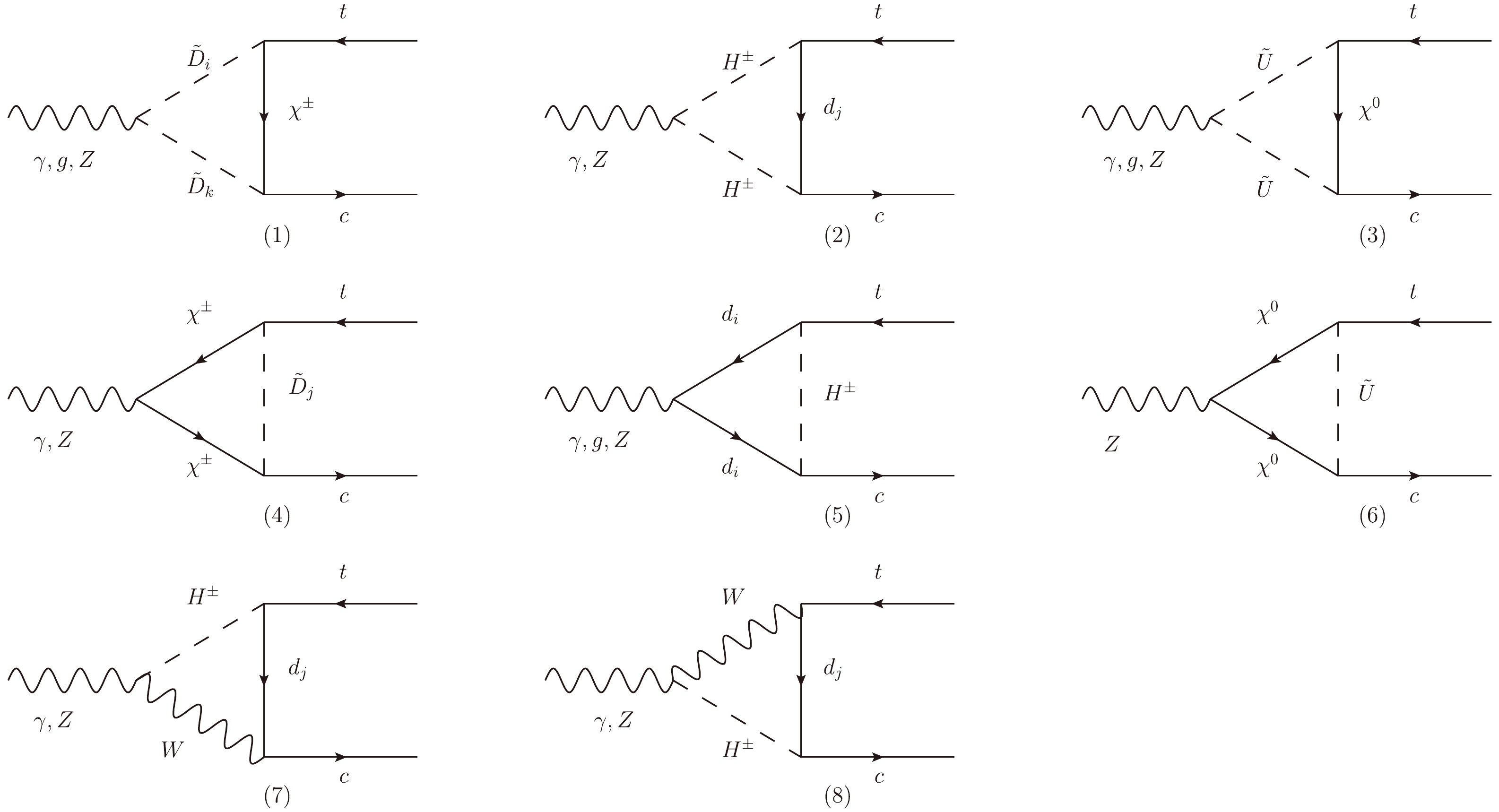
Figure 1. Feynman diagrams for the
$ t\rightarrow c\gamma $ ,$ t\rightarrow cg $ ,$ t\rightarrow cZ $ processes in the$ U(1)_X $ SSM.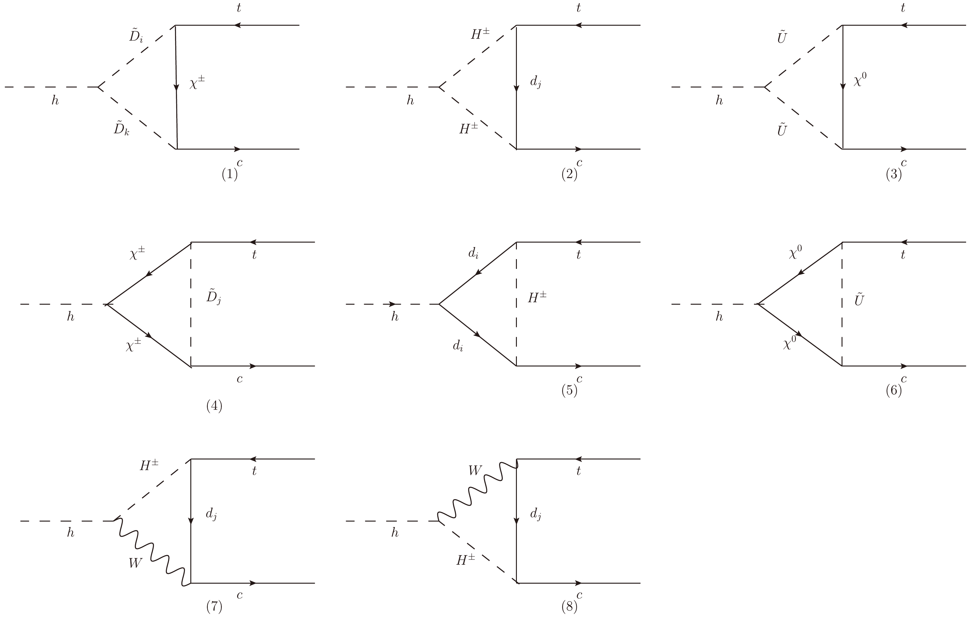
Figure 2. Feynman diagrams for the
$ t\rightarrow ch $ process in the$ U(1)_X $ SSM.In the
$ U(1)_X $ SSM, the flavor violating amplitude corresponding to the decay process$ t\rightarrow cV $ ($ V = \gamma, Z $ ) is expressed as follows:$ {\cal{M}}_{t\rightarrow cV} = \varepsilon^\mu\bar{u}_c(p')\Big(A_V\gamma_\mu P_L+iB_V\sigma_{\mu\nu}q^\nu P_L+(L\rightarrow R)\Big)u_t(p). $

(13) To better explain how the calculations of the above equation and Feynman diagrams in Fig. 1 are done, Fig. 1(1) is selected as an example. The corresponding amplitude can be expressed as follows:
$ \begin{aligned}[b] {\cal{M}}_{t\rightarrow cV} =\;& \sum\limits_{i,j,k,n}\varepsilon^\mu\bar{u}_c(p')\int\frac{{\rm d}^Dk}{(2\pi)^D} {\rm i} (A_{\bar{c}\tilde{D}_k\chi^\pm_n }^LP_L+A_{\bar{c}\tilde{D}_k\chi_n^\pm}^RP_R)\\&\times\frac{\rm i}{{\not {p}}-{\not {k}}-m_{\chi_n^\pm}} {\rm i} (A_{\bar{\chi}_n^\pm\tilde{D}_it}^LP_L+A_{\bar{\chi}_n^\pm\tilde{D}_it}^RP_R)\frac{\rm i}{k^2-m_{\tilde{D}_i}^2} {\rm i} B_{V\tilde{D}_i\tilde{D}_k}\\&\times(-2k_\mu+q_\mu) \frac{\rm i}{(k-q)^2-m_{\tilde{D}_k}^2}u_t(p). \end{aligned} $

(14) Here,
$ \varepsilon_\mu $ denotes the polarization vectors of the photon and Z boson;$ u_t $ and$ u_c $ denote the wave functions of the top and charm quarks; p is the momentum of the top quark;$ p' $ is the momentum of the charm quark; q is the momentum of the vector boson; and$ m_{\tilde{D}_i} $ ,$ m_{\tilde{D}_k} $ , and$ m_{\chi^\pm} $ are the mass eigenvalues from Eq. (9). Correspondingly,$ A_{\bar{c}\tilde{D}\chi^\pm}^L $ ,$ A_{\bar{c}\tilde{D}\chi^\pm}^R $ ,$ A_{\bar{\chi}^\pm\tilde{D}t}^L $ ,$ A_{\bar{\chi}^\pm\tilde{D}t}^R $ , and$ B_{V\tilde{D}\tilde{D}} $ are the coupling vertices [39, 40, 45, 46]. L and R in the subscripts denote the left-handed and right-handed parts, respectively. They can be derived from SARAH.Next, we solve the Feynman integral. The formula employed for the integration of the denominator is [47]
$ \frac{1}{ABC} = \int^1_0{\rm d}x\int^1_02y{\rm d}y\frac{1}{[(Ax+B(1-x))y+C(1-y)]^3}. $

(15) Calculating the integral in this manner can greatly increase the efficiency of numerical calculations. According to Eq. (15), we obtain:
$ \begin{aligned}[b]& \int^1_0{\rm d}x\int^1_02y{\rm d}y\Big\{\Big([({\not {p}}-{\not {k}})^2-m_{\chi^\pm_n}^2]x+(k^2-m_{\tilde{D}_i}^2)(1-x)\Big)y +\Big(({\not{ k}}-{\not{ q}})^2-m_{\tilde{D}_k}^2\Big)(1-y)\Big\}^{-3} \\ =\;& \int^1_0{\rm d}x\int^1_02y{\rm d}y\Big\{[k-pxy-q(1-y)]^2-[pxy+q(1-y)]^2+(p^2-m_{\chi^\pm_n}^2)xy -m_{\tilde{D}_i}^2(1-x)y+(q^2-m_{\tilde{D}_k}^2)(1-y)\Big\}^{-3}, \end{aligned} $ 
(16) where we apply
${\not {b}} = -{\not {p}} xy-{\not {q}}(1-y)$ ,${\not {k'}} = {\not {k}}+{\not {b}}$ , and J =$-[p^2(xy-x^2y^2)+q^2((1-y)-(1-y)^2)-2p\cdot qxy(1-y)-m_{\chi^\pm_n}^2xy-$ $ m_{\tilde{D}_i}^2(1-x)y- m_{\tilde{D}_k}^2(1-y)] $ to obtain the final form of the denominator in Eq. (14):$ \int^1_0{\rm d}x\int^1_02y{\rm d}y\frac{1}{(k^{'2}-J)^3}. $

(17) This type of substitution is also performed for the numerator in Eq. (14). We take all the diagrams in Fig. 1 and calculate the Feynman amplitudes for
$ t\rightarrow c\gamma $ ,$ t\rightarrow cg $ , and$ t\rightarrow cZ $ . Finally, we calculate the respective mode squares for the three processes.In the MSSM, the top quark decay
$ t\rightarrow ch $ is flavor-changing, where h is the lightest CP-even Higgs boson. Note that in Fig. 2, the new contribution of the down-type quarks, the mixing between the Higgs doublet and exotic single-line states$ \tilde{\eta}_{1,2} $ also affects$ t\rightarrow ch $ decay channel. We use the following calculation related to Fig. 2(4) as an example. The amplitude can be expressed as follows:$ \begin{aligned}[b] &{\cal{M}}_{t\rightarrow ch} \\=\;& -\bar{u}_c(p')\int\frac{{\rm d}^Dk}{(2\pi)^D}\frac{1}{[(k-q)^2-m_{\chi^\pm}^2](k^2-m_{\chi^\pm}^2)[(p-k)^2-m_{\tilde{D}_j}^2]} ,\\ &\cdot (A_{\bar{c}\chi^\pm\tilde{D}_j}^LP_L+A_{\bar{c}\chi^\pm\tilde{D}_j }^RP_R)({\not{ k}}-{\not{ q}}+m_{\chi^\pm})(A_{\bar{\tilde{D}}_j^\dagger\chi^\pm t}^LP_L+A_{\bar{\tilde{D}}_j^\dagger\chi^\pm t}^RP_R)\\&\cdot({\not{ k}}+m_{\chi^\pm})(A_{h\chi^\pm\chi^\pm }^LP_L+A_{h\chi^\pm\chi^\pm }^RP_R)u_t(p). \\[-15pt]\end{aligned} $

(18) Other graphs of the
$ t\rightarrow ch $ process can be calculated similarly.We use dimensional regularization to treat the divergences with
$ d = 4-2\epsilon $ and the limit$ d\rightarrow4 $ . To obtain finite results, the divergences are canceled by the modified minimal substraction$ (\overline{MS}) $ scheme. The terms proportional to$ \frac{1}{\epsilon}-\gamma_E+\log(4\pi) $ are deleted. Here,$ \gamma_E\approx0.5772 $ is an Euler constant.Based on the above calculations, the branching ratios of the top-quark rare decays are respectively:
$ \begin{aligned}[b]& Br(t\rightarrow cV) = \frac{|{\cal{M}}_{tcV}|^2 \sqrt{((m_t+m_V)^2-m_c^2)((m+t-m_V)^2-m_c^2)}}{32\pi m_t^3\Gamma_{\rm total}},\\& Br(t\rightarrow ch) = \frac{|{\cal{M}}_{tch}|^2 \sqrt{((m_t+m_h)^2-m_c^2)((m+t-m_h)^2-m_c^2)}}{32\pi m_t^3\Gamma_{\rm total}}, \end{aligned} $

(19) where
$\Gamma_{\rm total}$ =$ 1.42_{-0.15}^{+0.19} $ $ {\rm{GeV}} $ [17] is the total decay width of the top quark. -
In this section, we study the numerical results of flavor violation for the top-quark
$ t\rightarrow cV, ch $ processes. According to the latest LHC data [48−52], our values are subject to certain constraints. Thus, we consider the following individual experimental constraints:1. The lightest CP-even Higgs mass is approximately 125.25 GeV [17, 53−55].
2. The updated experimental data show that the mass of the
$ Z' $ boson at the 95% confidence level (CL) [56] satisfies$ M_{Z'}> $ 5.15 TeV. Eq. (15) yields an approximate result of$ M_{Z'} $ as$ M_{Z'}\approx g_X\xi> $ 5.15 TeV.3. The ratio between
$ M_{Z'} $ and its gauge coupling constant is$ \dfrac{M_{Z'}}{g_X} \geqslant $ 6${\rm{TeV}} $ [57, 58]. Thus,$ g_X $ is restricted in the region 0$ <g_X\leqslant $ 0.85.4. The new angle
$ \beta_\eta $ is constrained by LHC as$ \tan\beta_\eta<1.5 $ [59].5. The limitations for the particle masses according to the PDG [17] data and the specific contents are as follows. The neutralino mass mandatorily exceeds 116 GeV, the chargino mass mandatorily exceeds 1000 GeV, and the scalar quark mass is greater than 1300 GeV.
The relevant SM input parameters in the numerical program were selected as follows:
$ m_Z $ = 91.188$ {\rm{GeV}} $ ,$ m_W $ = 80.385$ {\rm{GeV}} $ ,$ m_c $ = 1.27$ {\rm{GeV}} $ , and$ m_t $ = 172.69$ {\rm{GeV}} $ . In conjunction with the aforementioned experimental requirements, we obtained a wealth of data, and used graphs to analyze and process the data. We generally set the values of new particle masses ($ M_{BB'},\; M_{BL} $ ) in the order of$ 10^3 $ GeV, which is approximately the energy scale of new physics.$ T_{\lambda_C} $ and$ T_{\lambda_H} $ are trilinear coupling coefficients whose values are in the order of magnitude of the mass, and can be varied up or down to the order of$ 10^2 $ $ \sim $ $ 10^4 $ GeV.$ M_{Uii}^2 $ ,$ M_{Qii}^2 $ ,$ M_{Dii}^2 $ ,$ B_S $ , and$ B_\mu $ are all of mass square dimension, and can reach the order of$ 10^6 $ GeV$ ^2 $ . The dimensionless parameters$ \lambda_C $ and$ \lambda_H $ are generally set to values less than 1. Considering the constraints just described, we set the values of parameters as follows:$ \begin{aligned}[b]& M_{BB'} = 400\; {{\rm{GeV}}},\; M_{Uii}^2 = 6\times10^6\; {{\rm{GeV}}^2} (i = 1,2,3),\\& T_{\lambda_C} = -100\; {{\rm{GeV}}},\; M_{BL} = 1000\; {{\rm{GeV}}},\; \\&\lambda_C = -0.08,\; T_{\lambda_H} = 300\; {{\rm{GeV}}},\; \kappa = 0.1,\\& l_W = 4\times10^6\; {{\rm{GeV}}^2},\; B_\mu = B_S = 1\times10^6\; {{\rm{GeV}}^2}. \end{aligned}$

(20) We set the non-diagonal elements of the mass matrix to zero unless otherwise specified. In the
$ U(1)_X $ SSM,$ g_{YX} $ denotes the mixing gauge coupling constant of the$ U(1)_Y $ and$ U(1)_X $ groups; it is the parameter beyond MSSM. The mass matrices of neutralino, down type squark, and up type squark all contain$ g_{YX} $ . Furthermore,$ g_{YX} $ appears in the vertex and can enlarge its coupling constant.$ M_{BB'} $ is the mass of the$ U(1)_Y $ and$ U(1)_X $ gaugino mixings; it is present in the mass matrix of the neutralino. Moreover,$ \tan\beta $ appears in almost all the mass matrices of fermions, scalars, and Majoranas. It must be a sensitive parameter that affects the masses of particles and vertex couplings by directly influencing$ v_u $ and$ v_d $ ,$ M_{BL} $ is the mass of the new gaugino. It influences the mass matrix of the neutralino. Finally,$ \lambda_H $ relates to the strength of the self-interaction coupling of the Higgs field, which affects the VEV and Higgs boson mass. -
To determine the parameters affecting the top-quark flavor violation, some sensitive parameters need to be studied. To show the numerical results clearly, the parameters were set as follows:
$ M_{Dii}^2 = 6\times10^6\; {{\rm{GeV}}^2} $ ,$ M_{Qii}^2 = 6\times 10^6\; {{\rm{GeV}}^2} $ (i = 1,2,3),$ \mu = 1000\; {{\rm{GeV}}} $ ,$ M_1 = 1200\; {{\rm{GeV}}} $ . We next show plots depicting the relationship between Br($ t\rightarrow c\gamma $ ) and different parameters.First, we show one-dimensional diagrams of
$ Br(t\rightarrow c\gamma) $ versus$ M_{Q23}^2 $ ,$ M_2 $ in Fig. 3. The gray shaded area is the experimental limit satisfied by the$ Br(t\rightarrow c\gamma) $ process. Fig. 3(a) shows$ Br(t\rightarrow c\gamma) $ versus$ M_{Q23}^2 $ , with$ \tan\beta = 20 $ ,$ M_2 = 1200\; {{\rm{GeV}}} $ ,$ g_{YX} = 0.2 $ , and$ \lambda_H = 0.1 $ . The solid line corresponds to$ g_{X} $ = 0.3 whereas the dashed line corresponds to$ g_{X} $ = 0.6. Overall, both lines show a decreasing trend in the range of$ 0-4\times10^5\; {{\rm{GeV}}^2} $ for$ M_{Q23}^2 $ owing to the fact that the contribution of the lower-type squarks is canceled by the contribution of the charged Higgs boson at the turning point. Then, it is followed by an upward trend, which means that$ Br(t\rightarrow c\gamma) $ increases as$ M_{Q23}^2\geq4\times10^5\; {{\rm{GeV}}^2} $ . From bottom to top in Fig. 3 (a),$ Br(t\rightarrow c\gamma) $ increases as the value of$ g_{X} $ increases. Fig. 3 (c) shows the differential distribution of Fig. 3 (a). Figure 3 (c) further evidences the trend and pattern of the values in Fig. 3 (a). Moreover, in Fig. 3 (c), the differential increases linearly, and the speed of variable change is relatively smooth. This means that$ M_{Q23}^2 $ is a parameter that influences$ Br(t\rightarrow c\gamma) $ .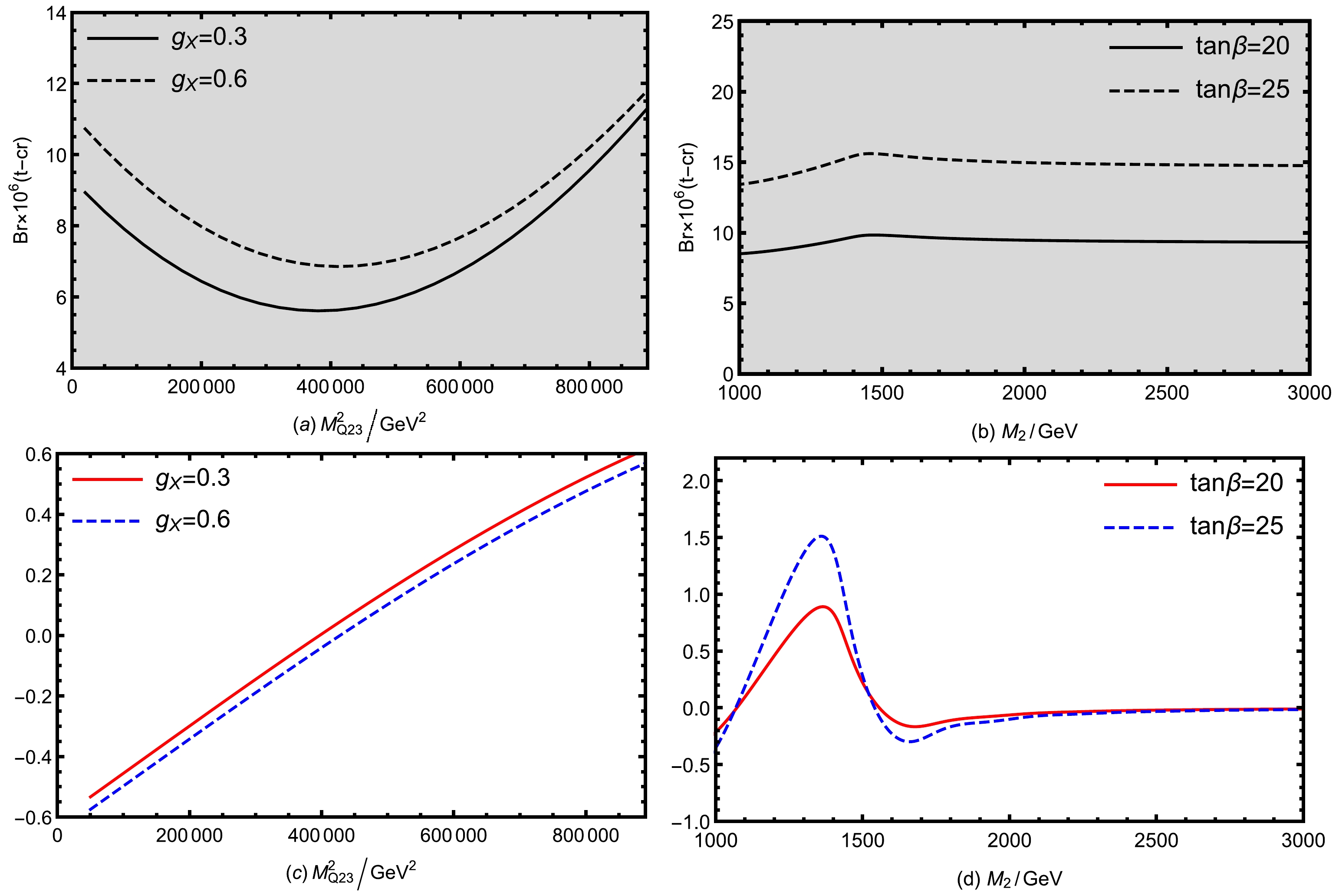
Figure 3. (color online) Diagrams of Br(
$ t\rightarrow c\gamma $ ) affected by different parameters. The gray area represents a reasonable value range where Br($ t\rightarrow c\gamma $ ) is lower than the upper limit. The solid and dashed lines in Fig. 3(a) correspond to$ g_{X} = 0.3 $ and$ g_{X} = 0.6 $ . The solid and dashed lines in Fig. 3(b) correspond to$ \tan\beta = 20 $ and$ \tan\beta = 25 $ , as$ M_{Qij} = 10^5 \; {{\rm{GeV}}^2} $ $ (i = j = 1,2,3, i\neq j) $ . Fig. 3(c) shows the differential distribution of (a) and Fig. 3(d) shows the differential distribution of (b).Figure 3 (b) represents
$ Br(t\rightarrow c\gamma) $ versus$ M_2 $ , with$ M_{Qij}^2 = 10^5\; {{\rm{GeV}}^2} $ $ (i,j = 1,2,3, i\neq j) $ ,$ g_X = 0.3 $ ,$ \lambda_H = 0.1 $ , and$ g_{YX} = 0.2 $ . The solid line corresponds to$ \tan\beta = 20 $ , whereas the dashed line corresponds to$ \tan\beta = 25 $ . There is a slight bulge in the$ Br(t\rightarrow c\gamma) $ value at$M_2 = 1400 {{\rm{GeV}}}$ , followed by a slight downward trend. It can be seen that the overall value satisfies this limit and follows a decreasing trend. As the line in the graph goes from bottom to top, i.e., as$ \tan\beta $ increases,$ Br(t\rightarrow c\gamma) $ also increases gradually. Figure 3 (d) shows the differential distribution of Fig. 3 (b). In Fig. 3 (d), there is a maximum of the differential value at$ M_2 $ = 1400 GeV; at this point,$ Br(t\rightarrow c\gamma) $ reaches its maximum value. The differential value is negative for$ M_2> $ 1600 GeV. That is to say,$ Br(t\rightarrow c\gamma) $ decreses, but very slightly.For a deeper exploration of the parameter space at
$ M_2 = 1200\; {{\rm{GeV}}} $ , we scanned some parameters randomly. In particular, in the$ Br(t\rightarrow c\gamma) $ process, we swept some parameters as follows:$ \begin{aligned}[b]& 5\leq\tan\beta\leq50,\; \; 0.3\leq g_X\leq0.7,\; \; \\&0.01\leq g_{YX}\leq0.5,\; \; 0.1\leq \lambda_H\leq0.4. \end{aligned} $

(21) In Fig. 4(a), we set
$ \lambda_H = 0.1 $ and$ g_{YX} = 0.2 $ to explore the effects of$ \tan\beta $ and$ g_{X} $ on$ Br(t\rightarrow c\gamma) $ . It is clear from this figure that the value of$ Br(t\rightarrow c\gamma) $ increases as$ \tan\beta $ increases. When$ \tan\beta $ reaches its maximum value of 50,$ Br(t\rightarrow c\gamma) $ reaches an order of magnitude of$ 10^{-4} $ , very close to the experimental upper limit. This indicates that$ \tan\beta $ is a crucial parameter. The value of$ Br(t\rightarrow c\gamma) $ becomes large as$ g_{X} $ increases; however, the effect of$ g_{X} $ on$ Br(t\rightarrow c\gamma) $ is small and hardly noticeable.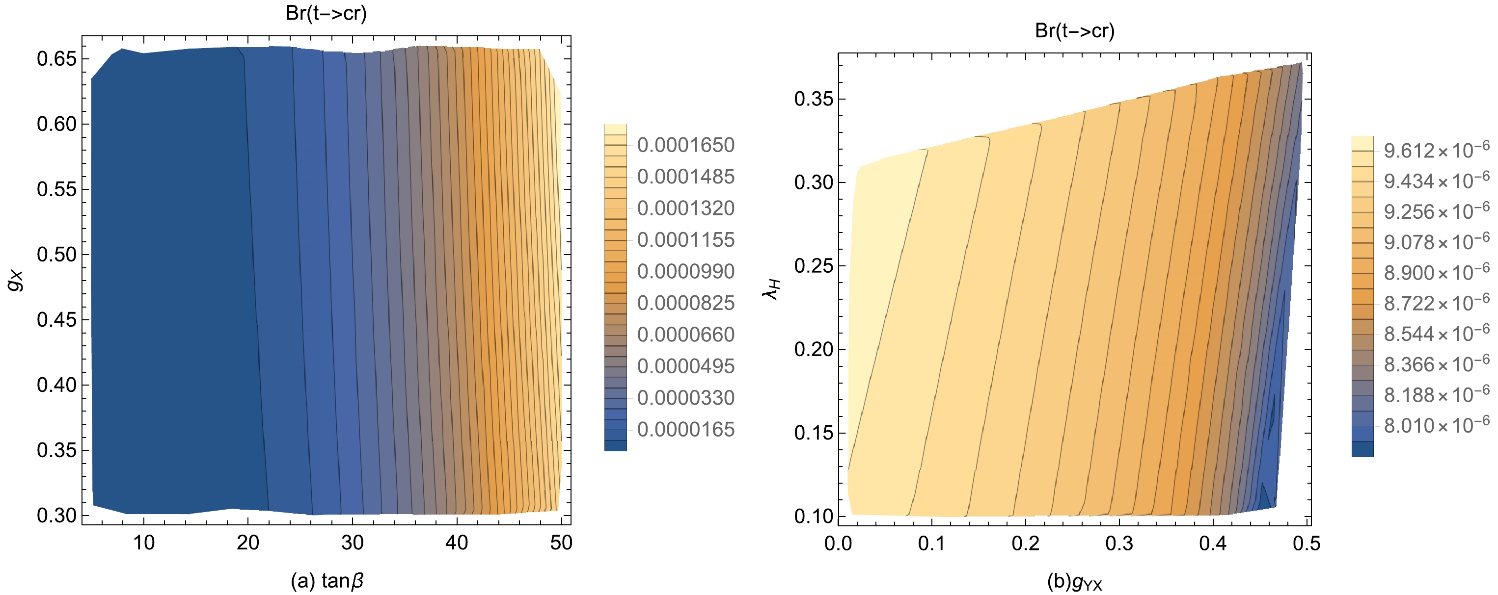
Figure 4. (color online) (a) Effects of
$ \tan\beta $ and$ g_X $ on$ Br(t\rightarrow c\gamma) $ . The horizontal coordinate indicates the range$ 5\leq\tan\beta\leq50 $ whereas the vertical coordinate indicates the range$ 0.3\leq g_X\leq0.7 $ . (b) Effects of$ g_{YX} $ and$ \lambda_H $ on$ Br(t\rightarrow c\gamma) $ . The horizontal coordinate indicates the range$ 0.01\leq g_{YX}\leq0.5 $ whereas the vertical coordinate indicates$ 0.1\leq \lambda_H\leq0.4 $ . The icons on the right side indicate the colors corresponding to the values of$ Br(t\rightarrow c\gamma) $ .In Fig. 4(b), we set
$ \tan\beta = 20 $ and$ g_{X} = 0.3 $ to explore the effects of$ \lambda_H $ and$ g_{YX} $ on$ Br(t\rightarrow c\gamma) $ . Note that both$ \lambda_H $ and$ g_{YX} $ have effects on$ Br(t\rightarrow c\gamma) $ . The value of$ Br(t\rightarrow c\gamma) $ decreases with the increase of$ g_{YX} $ . The smaller the value of$ g_{YX} $ , the closer to the upper limit of$ Br(t\rightarrow c\gamma) $ . There is a slight increase in the value of$ Br(t\rightarrow c\gamma) $ with$ \lambda_H $ , but the impact of$ \lambda_H $ is relatively small compared to that of$ g_{YX} $ . Figure 4(b) shows the presence of a white area in the upper left corner. This is due to the limitation established by the masses of Higgs and other particles. -
In this section, we continue our exploration of the branching ratio of
$ t\rightarrow cg $ with respect to certain parameters. In this case, we set$ M_1 = 1200\; {{\rm{GeV}}} $ ,$ M_2 = 1200\; {{\rm{GeV}}} $ ,$ M_{Dii}^2 = 6\times10^6\; {{\rm{GeV}}^2} $ , and$ M_{Qii}^2 = 6\times10^6\; {{\rm{GeV}}^2} $ . One-dimensional diagrams of Br($ t\rightarrow cg $ ) are shown in Fig. 5. The gray shaded portion indicates the experimental limit that is satisfied by the Br($ t\rightarrow cg $ ) process. Figure 5 (a) shows Br($ t\rightarrow cg $ ) versus$ M_{U23}^2 $ for$ \tan\beta = 20 $ ,$ \lambda_H $ = 0.1,$ g_{X} = 0.3 $ , and$ g_{YX} = 0.2 $ ; the solid and dashed lines correspond to$ \mu = 1000\; {{\rm{GeV}}} $ and$ \mu = 1100\; {{\rm{GeV}}} $ , respectively. Note that Br($ t\rightarrow cg $ ) increases with$ M_{U23}^2 $ and the value approaches the experimental upper limit as$ M_{U23}^2 $ further increases. Note also that Br($ t\rightarrow cg $ ) decreases as μ increases. Figure 5 (c) shows the differential distribution of Fig. 5 (a). According to Fig. 5 (c), the variation of Fig. 5(a) is mostly regular. Note that$ t\rightarrow cg $ increases with$ M_{U23}^2 $ .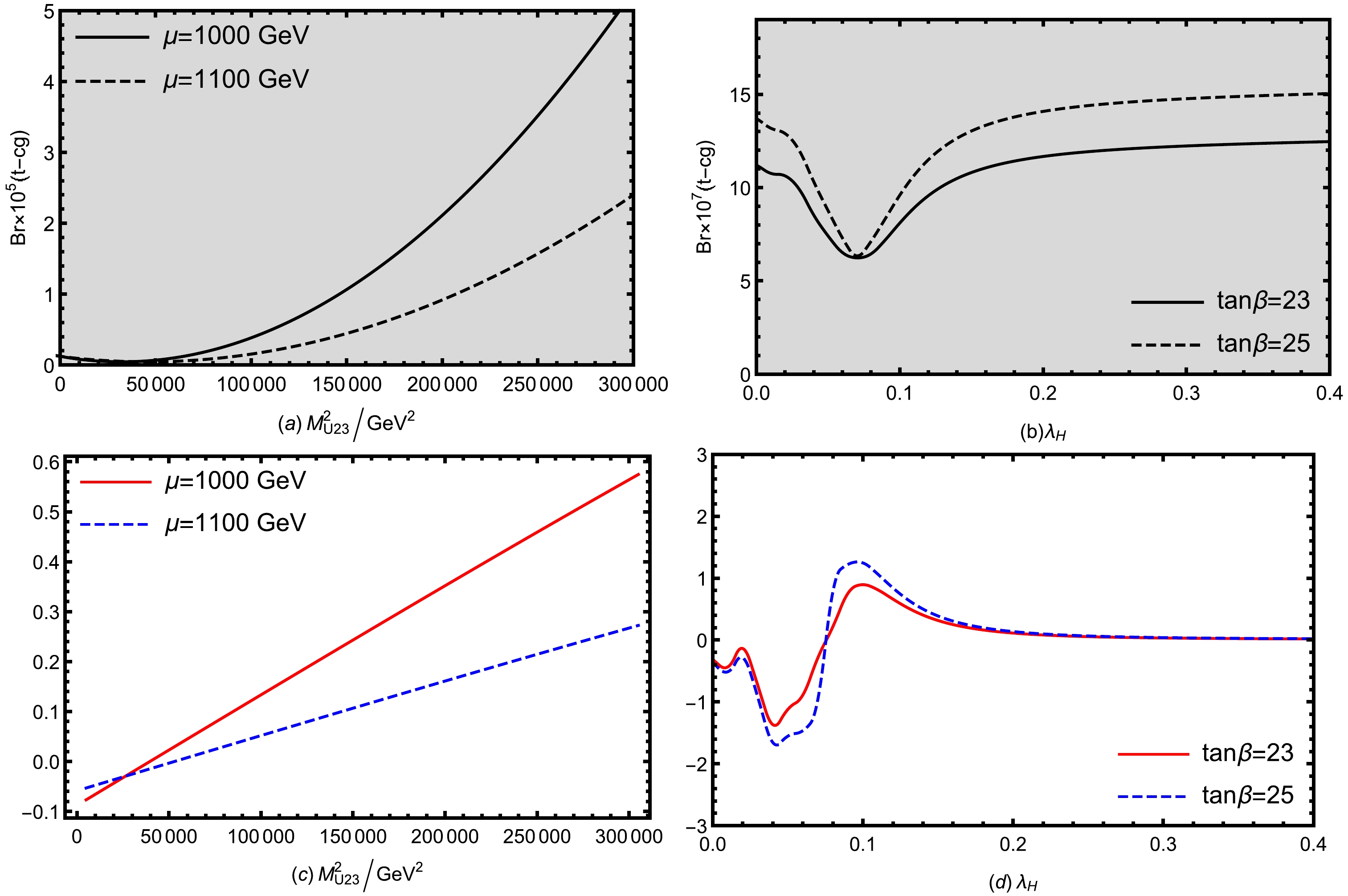
Figure 5. (color online) Br(
$ t\rightarrow cg $ ) diagrams affected by different parameters. The gray area represents a reasonable value range where Br($ t\rightarrow cg $ ) is lower than the upper limit. The solid and dashed lines in Fig. 5(a) correspond to$ \mu = 1000\; {{\rm{GeV}}} $ and$ \mu = 1100\; {{\rm{GeV}}} $ . The solid and dashed lines in Fig. 5(b) correspond to$ \tan\beta = 23 $ and$ \tan\beta = 25 $ . Fig. 5(c) shows the differential distribution of (a) and Fig. 5(d) shows the differential distribution of (b).Figure 5 (b) shows Br(
$ t\rightarrow cg $ ) versus$ \lambda_H $ with$M_{Q23} = 10^5 {{\rm{GeV}}^2}$ ,$ \mu = 1000\; {{\rm{GeV}}} $ ,$ g_{X} = 0.3 $ ,$ g_{YX} = 0.2 $ ,$ \tan\beta = 23 $ (solid line), and$ \tan\beta = 25 $ (dashed line). Note that the value of Br($ t\rightarrow cg $ ) shows a minimum at$ \lambda_H = 0.08 $ , which is due to the mixing of several parameters. Its overall value satisfies the experimental limit of the process; it is from five to six orders of magnitude higher than the SM prediction. As$ \tan\beta $ increases from 23 to 25, the Br($ t\rightarrow cg $ ) value also increases. However, note that the Br($ t\rightarrow cg $ ) values almost coincide at$ \lambda_H = 0.07 $ . Figure 5 (d) shows the differential distribution of Fig. 5 (b). In Fig. 5 (d), the differential values are negative for$ \lambda_H< $ 0.08, and Br($ t\rightarrow cg $ ) decreases as$ \lambda_H $ becomes larger. In the range$0.08\leq \lambda_H < 0.11$ , the slope is the largest, and Br($ t\rightarrow cg $ ) changes more quickly than the others. For$ \lambda_H\geq $ 0.11, the differential values are all positive, but the value variation is small. Moreover, Br($ t\rightarrow cg $ ) becomes larger, although the magnitude of the increase is smaller.Let us assume that
$ \mu = 1000\; {{\rm{GeV}}} $ and$ \lambda_H = 0.1 $ . We randomly scanned the parameters$ \tan\beta $ ,$ g_X $ ,$ g_{YX} $ as follows:$ 5\leq\tan\beta\leq50,\; \; 0.3\leq g_X\leq0.7,\; \; 0.01\leq g_{YX}\leq0.5. $

(22) In Fig. 6 (a), we set
$ g_X = 0.3 $ to explore the effects of$ \tan\beta $ and$ g_{YX} $ on$ Br(t\rightarrow cg) $ . Note that as$ \tan\beta $ increases,$ Br(t\rightarrow cg) $ gradually changes from blue to yellow, i.e., a significant increase in$ Br(t\rightarrow cg) $ occurs. The larger the value of$ \tan\beta $ , the closer the value of$ Br(t\rightarrow cg) $ to the experimental upper limit. Note that$ g_{YX} $ has some minor effect on the results, and this effect is hardly noticeable. In Fig. 6 (b), we set$ \tan\beta = 20 $ to explore the effects of$ g_{X} $ and$ g_{YX} $ on$ Br(t\rightarrow cg) $ ; note that the larger the value of$ g_{X} $ , the larger the value of$ Br(t\rightarrow cg) $ . Note also that the larger the value of$ g_{YX} $ , the smaller the value of$ Br(t\rightarrow cg) $ .$ Br(t\rightarrow cg) $ is maximized at$ g_{X} = 0.7 $ and$ g_{YX} = 0.01 $ , and$ Br(t\rightarrow cg) $ becomes closer to the upper limit of the experiment. When$ g_{YX} $ tends to zero, the dependence of the branching ratio on$ g_{X} $ is strong.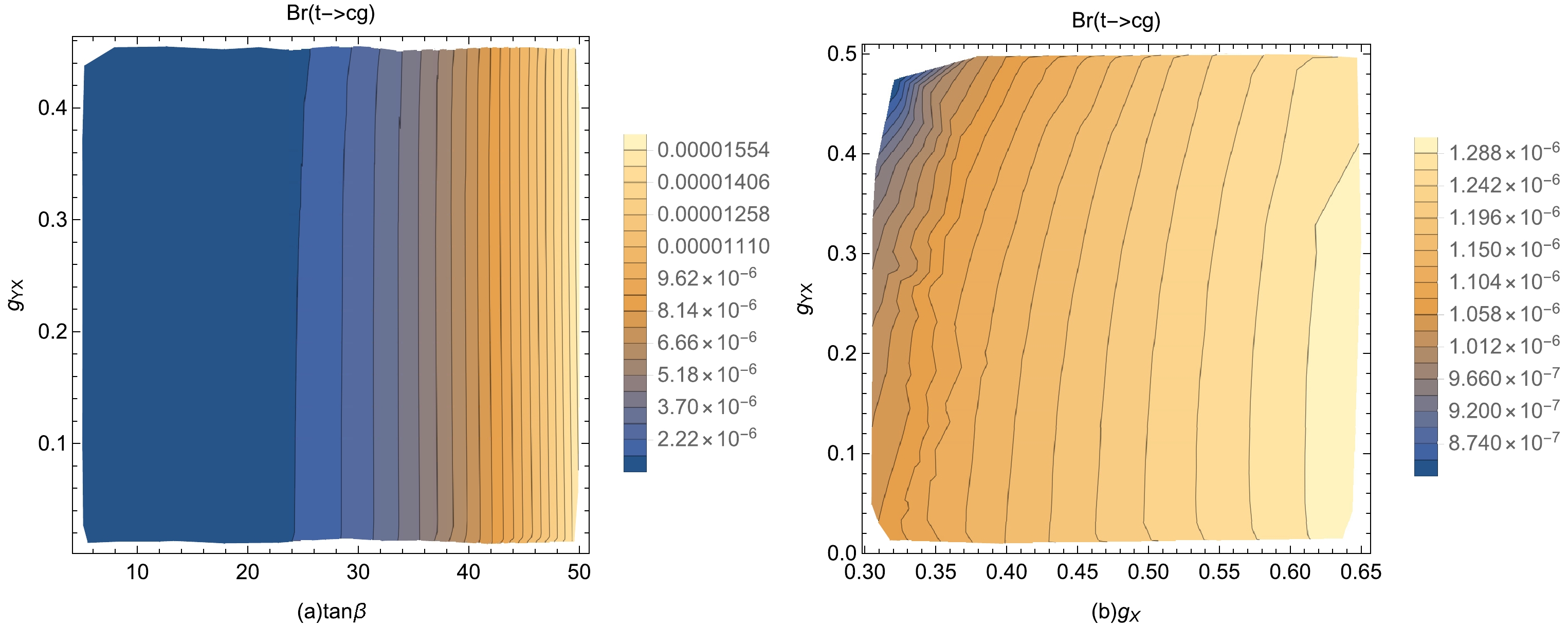
Figure 6. (color online) (a) Effects of
$ \tan\beta $ and$ g_{YX} $ on$ Br(t\rightarrow cg) $ . The horizontal coordinate indicates the range$ 5\leq\tan\beta\leq50 $ whereas the vertical coordinate indicates the range$ 0.01\leq g_{YX}\leq0.5 $ . (b) Effects of$ g_{X} $ and$ g_{YX} $ on$ Br(t\rightarrow cg) $ . The horizontal coordinate indicates the range$ 0.3\leq g_{X}\leq0.7 $ whereas the vertical coordinate indicates$ 0.01\leq g_{YX}\leq0.5 $ . The icons on the right side indicate the colors corresponding to the values of$ Br(t\rightarrow cg) $ . -
The experimental upper bound (
$ 5\times10^{-4} $ ) for the$ Br(t\rightarrow cZ) $ process is of the same order of magnitude as that for$ Br(t\rightarrow c\gamma) $ and$ Br(t\rightarrow cg) $ . In this subsection, we analyze the effects of different parameters on the$ Br(t\rightarrow cZ) $ branching ratio. In particular, we focus on the effects of the parameters$ M_{U23}^2 $ ,$ M_2 $ ,$ g_X $ ,$ g_{YX} $ ,$ M_{Dii}^2 $ , and$ M_{Qii}^2 $ . We set$ M_1 = 1200\; {{\rm{GeV}}} $ and$ \lambda_H = 0.1 $ . One-dimensional representations are presented in Fig. 7 whereas multi-dimensional plots are presented in Fig. 8.
Figure 7. (color online) Br(
$ t\rightarrow cZ $ ) diagrams affected by different parameters. The gray area indicates a reasonable value range where$ Br(t\rightarrow cZ) $ is lower than the upper limit. The solid and dashed lines in Fig. 7(a) correspond to$ \mu = 1000\; {{\rm{GeV}}} $ and$ \mu = 1500\; {{\rm{GeV}}} $ . The solid and dashed lines in Fig. 7(b) correspond to$ \tan\beta = 20 $ and$ \tan\beta = 25 $ . Fig. 7(c) shows the differential distribution of (a) and Fig. 7(d) shows the differential distribution of (b).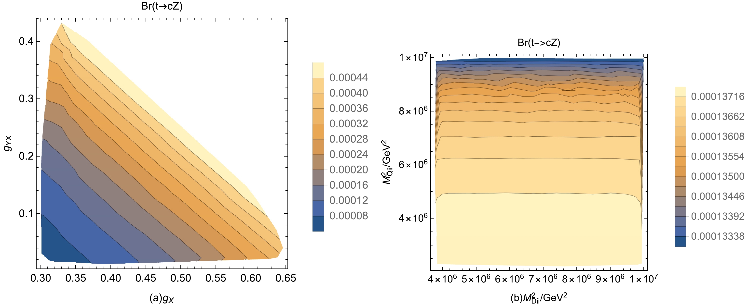
Figure 8. (color online) (a) Effects of
$ g_{X} $ and$ g_{YX} $ on$ Br(t\rightarrow cZ) $ . The horizontal coordinate indicates the range$ 0.3\leq g_{X}\leq0.7 $ whereas the vertical coordinate indicates$ 0.01\leq g_{YX}\leq0.5 $ . (b) Effects of$ M_{Dii}^2 $ and$ M_{Qii}^2 $ on$ Br(t\rightarrow cZ) $ . The horizontal coordinate indicates the range$ 10^6\; {{\rm{GeV}}^2}\leq M_{Dii}^2\leq10^7\; {{\rm{GeV}}^2} $ whereas the vertical coordinate indicates the range$ 10^6\; {{\rm{GeV}}^2}\leq M_{Qii}^2\leq10^7\; {{\rm{GeV}}^2} $ . The icons on the right side indicate the colors corresponding to the values of$ Br(t\rightarrow cZ) $ .Fig. 7(a) represents
$ Br(t\rightarrow cZ) $ versus$ M_{U23}^2 $ for$M_2 = 1200\; {{\rm{GeV}}}$ ,$ \tan\beta = 20 $ ,$ g_X = 0.3 $ ,$ g_{YX} = 0.2 $ ,$M_{Dii}^2 = 6\times 10^6\; {{\rm{GeV}}^2}$ , and$ M_{Qii}^2 = 6\times10^6\; {{\rm{GeV}}^2} $ , with the solid and dashed lines representing$ \mu = 1000\; {{\rm{GeV}}} $ and$\mu = 1500 {{\rm{GeV}}}$ , respectively. Note that both lines show an increasing trend, i.e.,$ Br(t\rightarrow cZ) $ increases with$ M_{U23}^2 $ . However, the change is not significant in terms of value. Note also a decrease in$ Br(t\rightarrow cZ) $ as μ increases. Both curves are shaded in gray. In Fig. 7 (b), we set$ \mu = 1000\; {{\rm{GeV}}} $ ,$g_X = 0.3$ ,$ g_{YX} = 0.2 $ ,$ M_{Dii}^2 = 6\times10^6\; {{\rm{GeV}}^2} $ , and$M_{Qii}^2 = 6\times10^6 {{\rm{GeV}}^2}$ ; the figure shows$ Br(t\rightarrow cZ) $ versus$ M_2 $ for$ \tan\beta = 20 $ (solid line) and$ \tan\beta = 25 $ (dashed line). The two lines are convex and reach a maximum at$ M_2 = 1150\; {{\rm{GeV}}} $ , then exhibit a downward trend and finally level off, i.e., in the range of$1000\; {{\rm{GeV}}}\leq M_2 \leq 1500\; {{\rm{GeV}}}$ ,$ M_2 $ has a clear influence on$ Br(t\rightarrow cZ) $ . The solid and dashed lines run from bottom to top, indicating that$ \tan\beta $ is also a sensitive parameter for$ Br(t\rightarrow cZ) $ , which increases with$ \tan\beta $ .Figure 7(c) shows the differential distribution of Fig. 7 (a). In Fig. 7 (c), the difference values are all positive. When
$ \mu = 1000\; {{\rm{GeV}}} $ and$ \mu = 1500\; {{\rm{GeV}}} $ , the difference between the values is very small, and the two lines almost coincide. Figure 7 (d) shows the differential distribution of Fig. 7 (b). In Fig. 7 (d), the differential values in most regions are negative when$ M_2 < 1500\; {{\rm{GeV}}} $ ; otherwise, they are positive.To further explore the effects of different parameters on
$ Br(t\rightarrow cZ) $ , we set$ \mu = 1000\; {{\rm{GeV}}} $ ,$ M_2 = 1200\; {{\rm{GeV}}} $ , and$ \tan\beta = 20 $ and performed randomized scans in the following ranges:$ \begin{array}{l} 0.01\leq g_{YX}\leq0.5,\; \; 10^6\; {{\rm{GeV}}^2}\leq M_{Dii}^2\leq10^7\; {{\rm{GeV}}^2},\\ 0.3\leq g_X\leq0.7,\; \; 10^6\; {{\rm{GeV}}^2}\leq M_{Qii}^2\leq10^7\; {{\rm{GeV}}^2}\; (i = 1,2,3). \end{array}$

(23) In Fig. 8 (a), we set
$ M_{Qii}^2 = 6\times10^6\; {{\rm{GeV}}^2} $ ,$M_{Dii}^2 = 6\times10^6\; {{\rm{GeV}}^2}$ to explore the effects of$ g_X $ and$ g_{YX} $ on$ Br(t\rightarrow cZ) $ . Note that$ Br(t\rightarrow cZ) $ has a minimum at$ g_X = 0.3 $ and$ g_{YX} = 0.01 $ . For$ Br(t\rightarrow cZ) $ , both$ g_X $ and$ g_{YX} $ are sensitive parameters;$ g_{YX} $ is a coupling constant that affects the strength of gauge mixing. Furthermore,$ g_X $ and$ g_{YX} $ make a new contribution to$ Br(t\rightarrow cZ) $ through$ Z-Z' $ mixing;$ g_X $ also affects significantly$ Br(t\rightarrow cZ) $ when$ g_{YX} $ tends to a minimum.$ Br(t\rightarrow cZ) $ increases with$ g_X $ and$ g_{YX} $ . In Fig. 8(a), the white region appears in the upper right corner. We conclude that it is excluded by the experimental upper limit, i.e.,$ Br(t\rightarrow cZ)<5\times10^{-4} $ .In Fig. 8 (b), we set
$ g_X = 0.3 $ and$ g_{YX} = 0.2 $ to explore the effects of$ M_{Qii}^2 $ and$ M_{Dii}^2 $ on$ Br(t\rightarrow cZ) $ . The values of$ M_{Qii}^2 $ and$ M_{Dii}^2 $ are both in the range of$10^6-10^7 {{\rm{GeV}}^2}$ . Fig. 8 (b) shows that$ M_{Dii}^2 $ has an extremely small effect on$ Br(t\rightarrow cZ) $ . However, as$ M_{Qii}^2 $ increases,$Br(t\rightarrow cZ)$ changes from yellow to blue, i.e.,$ Br(t\rightarrow cZ) $ decreases weakly as$ M_{Qii}^2 $ increases.In summary, regarding the
$ t\rightarrow cZ $ process, the main sensitive parameters are$ M_2 $ ,$ g_X $ ,$ g_{YX} $ , and the off-diagonal element$ M_{U23}^2 $ . The diagonal elements$ M_{Qii}^2 $ (i = 1,2,3) have an effect, but they are not particularly sensitive. -
The experimental upper bound for
$ Br(t\rightarrow ch) $ is$1.1\times 10^{-3}$ . In the$ U(1)_X $ SSM,$ Br(t\rightarrow ch) $ can be as high as$ 10^{-4} $ in some regions of the parameter space. Here, we set$ M_2 = 1200\; {{\rm{GeV}}} $ ,$ M_{Qii}^2 = 6\times10^6\; {{\rm{GeV}}^2} $ , and$M_{Dii}^2 = 6\times10^6 {{\rm{GeV}}^2}$ . We studied the effects of$ M_{Q23}^2 $ , μ,$ M_1 $ , and$ \tan\beta $ on$ Br(t\rightarrow ch) $ , as shown in Fig. 9. Figure 9 (a) shows$ Br(t\rightarrow ch) $ versus$ M_{Q23}^2 $ for$ g_X = 0.4 $ ,$ \mu = 1000\; {{\rm{GeV}}} $ ,$\tan\beta = 20$ ,$ g_{YX} = 0.2 $ , and$ \lambda_H = 0.1 $ . The solid line represents$ M_1 = 1200\; {{\rm{GeV}}} $ whereas the dashed line represents$ M_1 = 1600\; {{\rm{GeV}}} $ . As the dashed and solid lines go from bottom to top, it can be observed that$ M_2 $ has an effect on$ Br(t\rightarrow ch) $ as a sensitive parameter, and$ Br(t\rightarrow ch) $ decreases as$ M_2 $ increases. Note that$ Br(t\rightarrow ch) $ increases with$ M_{Q23}^2 $ almost linearly. Therefore,$ M_{Q23}^2 $ is also a parameter that notably affects$ Br(t\rightarrow ch) $ . Figure 9 (c) shows the differential distribution of Fig. 9 (a). In Fig. 9(c), the differential values are all positive. The trend of these values is relatively smooth and the regularity is more evident.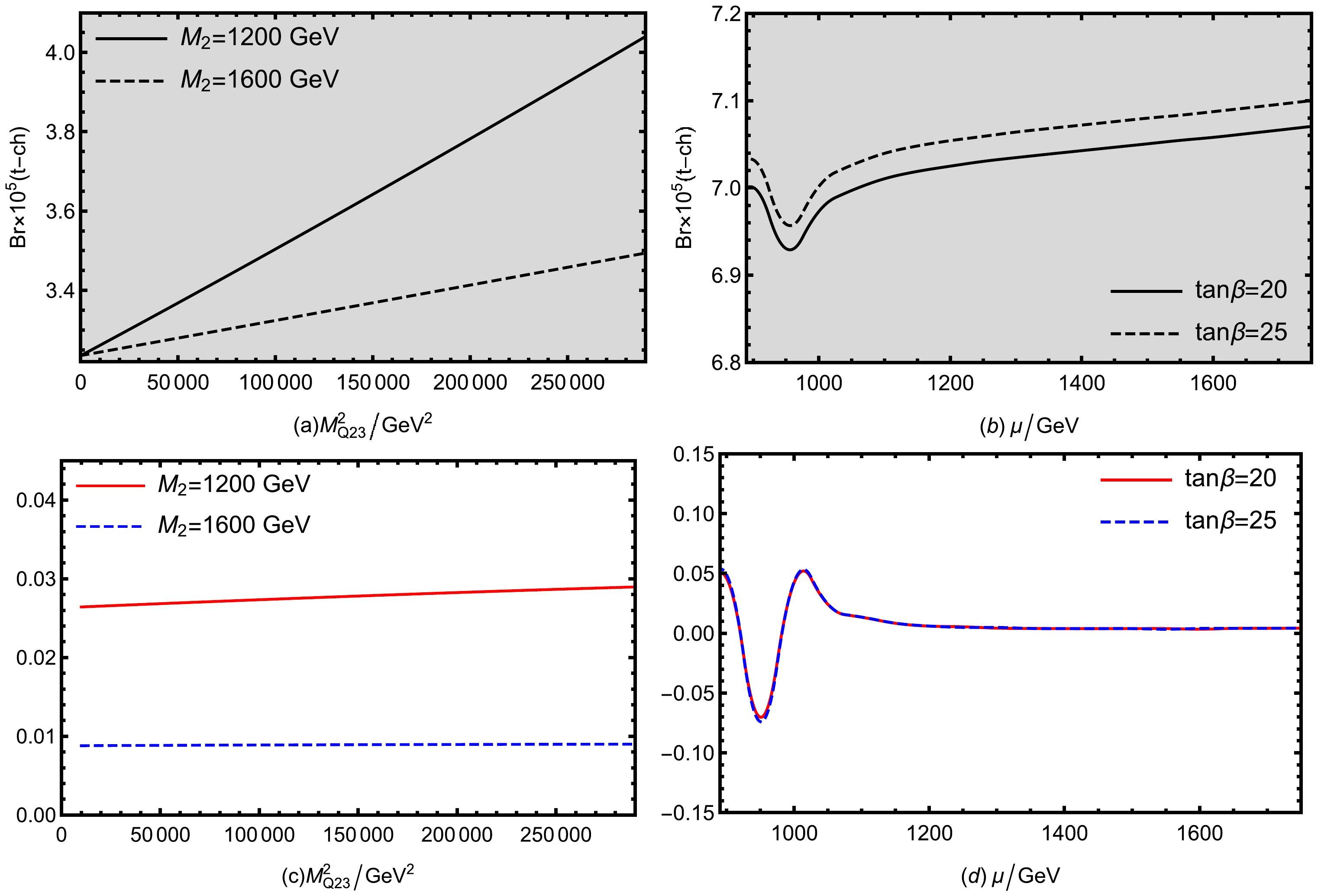
Figure 9. (color online) Br(
$ t\rightarrow ch $ ) diagrams affected by different parameters. The gray area indicates a reasonable value range where$ Br(t\rightarrow ch) $ is lower than the upper limit. For$ g_X = 0.4 $ , the solid and dashed lines in Fig. 9(a) correspond to$ M_1 = 1200\; {{\rm{GeV}}} $ and$ M_1 = 1600\; {{\rm{GeV}}} $ . Setting$ M_{Q23}^2 = 10^5\; {{\rm{GeV}}^2} $ , the solid and dashed lines in Fig. 9(b) correspond to$ \tan\beta = 20 $ and$ \tan\beta = 25 $ . Fig. 9(c) shows the differential distribution of (a) whereas Fig. 9(d) shows the differential distribution of (b).Figure 9 (b) shows
$ Br(t\rightarrow ch) $ versus μ for$M_1 = 1200\; {{\rm{GeV}}}$ ,$ g_{X} = 0.3 $ ,$ g_{YX} = 0.2 $ , and$ \lambda_H = 0.1 $ , with the solid line representing$ \tan\beta = 20 $ and the dashed line representing$ \tan\beta = 25 $ . By analyzing the three previous processes, i.e.,$ t\rightarrow c\gamma $ ,$ t\rightarrow cg $ and$ t\rightarrow cZ $ , we conclude that$ \tan\beta $ is one of the sensitive parameters. In the$ t\rightarrow ch $ process, Fig. 9 (b) shows that$ \tan\beta $ is a more sensitive parameter. When$ \tan\beta $ increases from 20 to 25,$ Br(t\rightarrow ch) $ increases with$ \tan\beta $ . It implies that$ Br(t\rightarrow ch) $ reaches a minimum at$ \mu = 950\; {{\rm{GeV}}} $ . When$ \mu>950\; {{\rm{GeV}}} $ ,$ Br(t\rightarrow ch) $ increases as μ increases, but the trend of increase is relatively small. Figure 9 (d) shows the differential distribution of Fig. 9 (b). In Fig. 9 (d), the differential values first decrease and then increase when$ \mu<1050\; {{\rm{GeV}}} $ . When$ \mu\geq1050\; {{\rm{GeV}}} $ , the tendency of these two lines to decrease becomes progressively weaker.To further explore the effect of other parameters on
$ Br(t\rightarrow ch) $ , we set$ M_1 = 1200\; {{\rm{GeV}}} $ ,$ \mu = 1000\; {{\rm{GeV}}} $ and performed a randomized scan of$ g_X $ ,$ g_{YX} $ ,$ \lambda_H $ , and$ \tan\beta $ :$\begin{aligned}[b]& 0.01\leq g_{YX}\leq0.5,\; \; 0.3\leq g_X\leq0.7,\; \; 0.1\leq\lambda_H\leq0.4,\\& 10\leq\tan\beta\leq50. \end{aligned} $

(24) Based on the parameters in Eq. (24), we obtained the data and plot depicted in Fig. 10. Figure 10(a) shows the effect of
$ g_{X} $ ($ 0.3\leq g_{X}\leq0.7 $ ) and$ g_{YX} $ ($ 0.01\leq g_{YX}\leq0.5 $ ) on$ Br(t\rightarrow ch) $ by setting$ \tan\beta = 20 $ ,$ \lambda_H = 0.1 $ . Fig. 10 (b) shows the effect of$ g_{X} $ ($ 0.3\leq g_{X}\leq0.7 $ ) and$\lambda_H\; (0.1\leq \lambda_H\leq0.4)$ on$ Br(t\rightarrow ch) $ by setting$ \tan\beta = 20 $ ,$ g_{YX} = 0.2 $ . In Fig. 10 (c), we set$ g_{X} = 0.3 $ and$ g_{YX} = 0.2 $ to explore the effect of$ \tan\beta\; (10\leq\tan\beta\leq50) $ and$\lambda_H\; (0.1 \leq \lambda_H\leq0.4)$ on$ Br(t\rightarrow ch) $ . Combining the three plots in Fig. 10, we can clearly see that the four parameters, i.e.,$ g_X $ ,$ g_{YX} $ ,$ \lambda_H $ , and$ \tan\beta $ , affect$ Br(t\rightarrow ch) $ , but they do so differently. Thus, both$ g_{X} $ and$ g_{YX} $ present clear effects on the numerical results.$ Br(t\rightarrow ch) $ is a decreasing function of$ g_{X} $ and$ g_{YX} $ . At the point they both reach their minimum value, the branching ratio of the$ t\rightarrow ch $ process reaches$ 10^{-4} $ , which is very close to the experimental upper limit. Figs. 10 (b) and (c) show that$ \lambda_H $ also behaves very sensitively, with$ Br(t\rightarrow ch) $ increasing as$ \lambda_H $ increases. Fig. 10 (c) shows that when$ \tan\beta>10 $ ,$ \tan\beta $ has a weak effect. This occurs because$ \tan\beta $ not only appears in the diagonal sectors of the mass matrix, but also dominates the non-diagonal sectors, leading to the above results.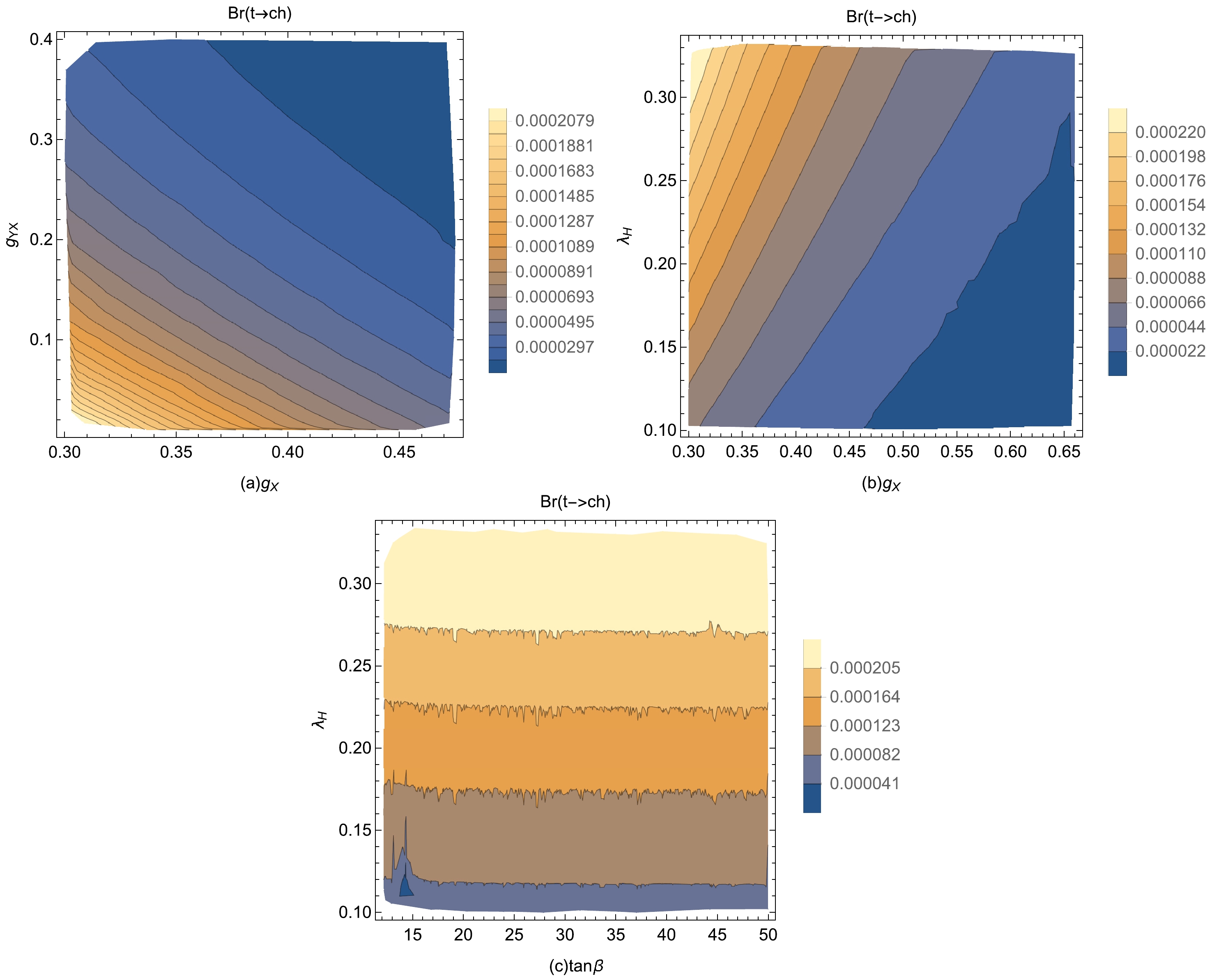
Figure 10. (color online) (a) Effects of
$ g_{X} $ and$ g_{YX} $ on$ Br(t\rightarrow ch) $ . The horizontal coordinate indicates the range$ 0.3\leq g_{X}\leq0.7 $ whereas the vertical coordinate indicates$ 0.01\leq g_{YX}\leq0.5 $ . (b) Effects of$ g_X $ and$ \lambda_H $ on$ Br(t\rightarrow ch) $ . The horizontal coordinate indicates the range$ 0.3\leq g_X\leq0.7 $ whereas the vertical coordinate indicates the range$ 0.1\leq\lambda_H\leq0.4 $ . (c) Effects of$ \tan\beta $ and$ \lambda_H $ on$ Br(t\rightarrow ch) $ . The horizontal coordinate indicates the range$ 5\leq \tan\beta\leq50 $ whereas the vertical coordinate indicates the range$ 0.1\leq\lambda_H\leq0.4 $ . The icons on the right side indicate the colors corresponding to the values of$ Br(t\rightarrow cZ) $ . -
In summary, we studied the rare decays
$t\rightarrow c\gamma, cg,\; cZ,\; ch$ of the top quark in the$ U (1)_X $ SSM. Compared to the MSSM, in the$ U(1)_X $ SSM we added three new Higgs singlets$ \hat{\eta},\; \hat{\bar{\eta}},\; \hat{S} $ and three generations of right-handed neutrinos$ \hat{\nu}_i $ . Its local gauge group is$S U(3)_C\times S U(2)_L \times U(1)_Y\times U(1)_X$ . Probing with the$ U(1)_X $ SSM made our study richer and more interesting, establishing a solid basis for the existence of new physics. We started with one-loop diagrams and computed the Feynman amplitude for each process to obtain numerical results for$ Br(t\rightarrow c\gamma),\; Br(t\rightarrow cg),\; Br(t\rightarrow cZ),\; Br(t\rightarrow ch) $ . We evaluated the effect of various parameters on the branching ratios of each process, selected the most illustrative results, and plotted one-dimensional and multi-dimensional plots for a more comprehensive numerical analysis based on experimental constraints.In the considered parameter space, numerical results show that all these processes are very close to the experimental upper limit, reaching even the same order of magnitude as the experimental upper limit at suitable parameter values. Therefore, they may be detected in future high-energy colliders. By analyzing the numerical results in the adopted parameter space, we can conclude that
$ \tan\beta $ ,$ g_X $ ,$ g_{YX} $ , μ,$ M_2 $ ,$ \lambda_H $ , and the off-diagonal parameters$ M_{U23}^2 $ ,$ M_{Q23}^2 $ are sensitive parameters that have a large influence on the branching ratios of the$ t\rightarrow c\gamma,\; cg,\; cZ,\; ch $ processes. Among them, the influence of$ \tan\beta $ is the greatest, being the main parameter of the$t\rightarrow c\gamma, cg,\; cZ,\; ch$ processes. Concerning$ \tan\beta $ , it appears in the mass matrixes of almost all SUSY particles. It is a fact that$ \tan\beta $ affects the numerical results mainly by influencing the particle masses, the corresponding rotational matrices, and the coupling vertexes. Regarding$ g_{YX} $ , it is a coupling constant in gauge mixing that is parameterized outside of the MSSM. In couplings where squarks appear,$ g_X $ and$ g_{YX} $ will affect the squark masses and corresponding rotation matrices, resulting in an effect on$Br(t\rightarrow c\gamma,\; cg,\; cZ,\; ch)$ . In addition, for the$ t\rightarrow cZ $ process, they generate new contributions via$ Z-Z' $ mixing. Comparing with the data in Table 3, we can see that the maximum value of$ Br(t\rightarrow cV, ch) $ obtained in the$ U(1)_X $ SSM is greater than that achieved in the B$ - $ LSSM. In particular, for$ Br(t\rightarrow ch) $ , the maximum value is even four orders of magnitude higher than that of the B$ - $ LSSM. The maximum of$ Br(t\rightarrow cV, ch) $ obtained in the$ U(1)_X $ SSM is already very close to the experimental upper limit, which makes our study more meaningful.Decay $ t\rightarrow c\gamma $ 

$ t\rightarrow cg $ 

$ t\rightarrow cZ $ 

$ t\rightarrow ch $ 

Upper limit (95%C.L.) $ 1.8\times10^{-4} $ 

$ 2\times10^{-4} $ 

$ 5\times10^{-4} $ 

$ 1.1\times10^{-3} $ 

$ B-L $ SSM [33]

$ 5\times10^{-7} $ 

$ 2\times10^{-6} $ 

$ 4\times10^{-7} $ 

$ 3\times10^{-9} $ 

$ U(1)_X $ SSM

$ 1.5\times10^{-4} $ 

$ 5\times10^{-5} $ 

$ 1.41\times10^{-4} $ 

$ 7.04\times10^{-5} $ 

Table 3. Upper limit (95%C.L.),
$ B-L $ SSM and$ U(1)_X $ SSM bounds on the decays$t\rightarrow cV, ch.$ In conclusion, we calculated the rare top-quark decays
$ t\rightarrow c\gamma,\; cg,\; cZ,\; ch $ in the$ U(1)_X $ SSM. They are certainly very interesting and worth exploring. Our study contributes to the understanding of the origin of R-parity and its possible spontaneous violation in super-symmetric models [60−62]. -
The authors thank Xi Wang, Yi-Tong Wang, Xin-Xin Long for participating in the discussion of the numerical results.
Top-quark rare decays with flavor violation
- Received Date: 2024-04-21
- Available Online: 2024-09-15
Abstract: In the present study, we investigated the decays of the top quark:


 DownLoad: