


 Abstract
 HTML
HTML Reference
 Related
 PDF
PDF


-
In 1998, at the Fermilab Tevatron, the CDF collaboration observed pseudoscalar
$ B_c $ mesons through the semi-leptonic decay modes$ B_c^{\pm} \to J/\psi \ell^{\pm}X $ and$ B_c^{\pm} \to J/\psi \ell^{\pm}\bar{\nu}_{\ell} $ in the$ p\bar{p} $ collisions at an energy of$ \sqrt{s}=1.8\,\rm{TeV} $ . The measured mass was$ 6.40 \pm 0.39 \pm 0.13 \,\rm{GeV} $ [1, 2]. This was the first time the bottom-charm meson was measured experimentally.In 2007, the CDF collaboration confirmed
$ B_c $ mesons through the non-leptonic decay modes$ B_c^{\pm} \to J/\psi \pi^{\pm} $ with a measured mass of$6275.6 \pm 2.9\pm 2.5 \; \rm{MeV}$ [3]. In 2008, the D0 collaboration reconstructed non-leptonic decays$B_c^{\pm} \to J/\psi \pi^{\pm}$ and confirmed$ B_c $ mesons with a measured mass of$ 6300 \pm 14 \pm 5\, \rm{ MeV} $ [4]. The$ B_c $ meson is now well established, and the average value listed in the Review of Particle Physics is$6274.47\pm 0.27\pm 0.17\;\rm{MeV}$ [5].In 2014, the ATLAS collaboration reported the observation of a structure in the
$ B_c^\pm \pi^+\pi^- $ invariant mass spectrum with a significance of 5.2 standard deviations, which is consistent with the predicted$ B_c^\prime $ meson with a mass of$ 6842\pm4\pm 5\, \rm{MeV} $ [6].In 2019, the CMS collaboration observed two excited
$ \bar{b}c $ states in the$ B^+_c\pi^+\pi^- $ invariant mass spectrum with a significance exceeding five standard deviations, which are consistent with$ B^{\prime+}_c $ and$ B_c^{*\prime+} $ , respectively [7]. The two states are separated in mass by$ 29.1 \pm 1.5 \pm 0.7 \, \rm{MeV} $ , and the mass of$ B^{\prime+}_c $ was measured to be$6871.0 \pm 1.2 \pm 0.8 \pm 0.8 \,\rm{ MeV}$ . Additionally, in 2019, the LHCb collaboration observed excited$ B^{\prime+}_c $ (with a global (local) statistical significance of$ 2.2\sigma $ ($ 3.2\sigma $ )) and$ B_c^{*\prime+} $ (with a global (local) statistical significance of$ 6.3\sigma $ ($ 6.8\sigma $ )) mesons in the$ B^+_c\pi^+\pi^- $ invariant mass spectrum. The$ B_c^{*\prime+} $ meson has a mass of$6841.2 \pm 0.6 \pm 0.1 \pm 0.8 \;\rm{MeV}$ , which is reconstructed without the low-energy photon emitted in$B_c^{*+} \to B_c^+ \gamma$ decay through the process$ B_c^{\prime*+} \to B_c^{*+} \pi^+ \pi^- $ , whereas the$ B^{\prime+}_c $ meson has a mass of$6872.1 \pm 1.3 \pm 0.1 \pm 0.8 \;\rm{MeV}$ [8].The
$ B_c^\prime $ meson emerging heavier than the$ B_c ^{*\prime} $ meson is an odd phenomenon as it conflicts with all the theoretical estimations. This may be owing to impossibility of reconstructing the low-energy photon in$ B_c ^{\ast +}\rightarrow B_c ^{+} \gamma $ decay [9]. More precise experimental data are required. Only the$ B_c $ and$ B_c^\prime $ mesons are listed in Review of Particle Physics [5], which is in contrast to the well-established spectroscopy of the charmonium and bottomonium states. Despite the significant developments in heavy quark physics in recent years, the bottom-charm spectroscopy remains poorly known. Thus, further investigations are required.Beauty-charm mesons provide an optimal platform for exploring both the perturbative and nonperturbative dynamics of heavy quarks, owing to the absence of contamination from the light quark, and for exploring the strong and electro-weak interactions. This is because they are composed of two different heavy flavor quarks and cannot annihilate into gluons or photons. The excited
$ c \bar b $ states, which lie below the$ BD $ threshold, would decay into the$ B_c $ meson through radiative or hadronic decays [10, 11]. In contrast, the ground state$ B_c $ can only decay weakly through emitting a virtual W-boson; thus, it cannot decay through strong or electromagnetic interactions.Several theoretical studies have been conducted on the mass spectroscopy of bottom-charm mesons, such as the relativized (or relativistic) quark model with a special potential [10−14], nonrelativistic quark model with a special potential [15−23], semi-relativistic quark model using the shifted large-N expansion [24, 25], perturbative QCD [26], nonrelativistic renormalization group [27], lattice QCD [28−31], Bethe-Salpeter equation [32−34], full QCD sum rules [35−41], and potential model combined with the QCD sum rules [15, 16].
With the continuous developments in experimental techniques, we expect that more
$ c\bar b $ states would be observed by collaborations and facilities such as ATLAS, CMS, and LHCb in the future. The decay constant, which parameterizes the coupling between a current and meson, is essential in exploring the exclusive processes. This is because the decay constants are not only fundamental parameters describing the pure leptonic decays but are also universal input parameters related to the distribution amplitudes, form-factors, partial decay widths, and branching fractions in many processes. By precisely measuring the branching fractions, we can utilize the decay constants to extract the CKM matrix element in the standard model and search for new physics beyond the standard model [42].Decay constants of the bottom-charm mesons have been investigated using several theoretical approaches, such as the full QCD sum rules [35−41, 43, 44], potential model combined with the QCD sum rules [15, 16], QCD sum rule combined with the heavy quark effective theory [45−52], covariant light-front quark model [53, 54], lattice non-relativistic QCD [31], shifted large-N expansion method [25], and field correlator method [55]. However, as the values from different theoretical approaches vary significantly, we are motivated to extend our previous works on vector and axialvector
$ B_c $ mesons [40] to investigate pseudoscalar and scalar$ B_c $ mesons with the full QCD sum rules by including next-to-leading order radiative corrections and using the updated input parameters. Thus, our investigations are performed consistently and systematically. We use experimental data [5−8] as guides in selecting suitable Borel parameters and continuum threshold parameters and examine the masses and decay constants of pseudoscalar and scalar$ B_c $ . mesons with the full QCD sum rules. Therefore, we calculate the pure leptonic decay widths to be compared with experimental data in the future.The remainder of this article is arranged as follows: we calculate the next-to-leading order contributions to the spectral densities and obtain the QCD sum rules in Sec. II. In Sec. III, we present the numerical results and discussions. Sec. IV provides our conclusions.
-
First, we express the two-point correlation functions:
$ \Pi_{P/S}(p^2)= {\rm i}\int {\rm d}^4x {\rm e}^{{\rm i} p \cdot x} \langle 0|T\left\{J(x)J^{\dagger}(0)\right\}|0\rangle \, , $

(1) where
$ J(x)=J_P(x) $ and$ J_S(x) $ are$ \begin{aligned}[b] J_P(x)=\;&\bar{c}(x){\rm i}\gamma_5 b(x)\, , \\ J_S(x)=\;&\bar{c}(x) b(x)\, , \end{aligned} $

(2) the subscripts P and S represent the pseudoscalar and scalar mesons, respectively. The correlation functions can be expressed in the form
$ \Pi_{P/S}(p^2)=\frac{1}{\pi}\int_{(m_b+m_c)^2}^\infty {\rm d} s \frac{{\rm Im\Pi}_{P/S}(s)}{s-p^2}\, , $

(3) according to the dispersion relation, where
$ \begin{aligned}[b] \frac{{\rm Im}\Pi_{P/S}(s)}{\pi}=\;&\rho_{P/S}(s) \\ =\;&\rho^0_{P/S}(s)+\rho^1_{P/S}(s)+\rho^2_{P/S}(s)+\cdots\, , \end{aligned} $

(4) the QCD spectral densities
$ \rho_{P/S}(s) $ are expanded in terms of the strong fine structure constant$ \alpha_s=\dfrac{g_s^2}{4\pi} $ .$ \rho^0_{P/S}(s) $ ,$ \rho^1_{P/S}(s) $ ,$ \rho^2_{P/S}(s) $ ,$ \cdots $ are the spectral densities of the leading order, next-to-leading order, and next-to-next-to-leading order,$ \cdots $ . At the leading order,$ \rho^0_{P/S}(s)= \frac{3}{8\pi^2}\frac{\sqrt{\lambda(s,m_b^2,m_c^2)}}{s}\left[s-(m_b\mp m_c)^2 \right]\,, $

(5) where the standard phase space factor is
$ \lambda(s,m_b^2,m_c^2)=s^2+m_b^4+m_c^4-2sm_b^2-2sm_c^2-2m_b^2m_c^2\, . $

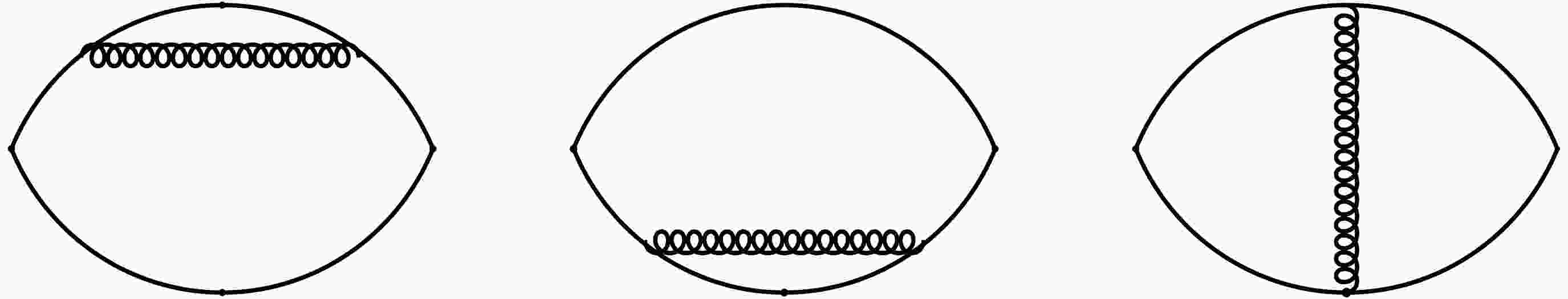
(6) At the next-to-leading order, three standard Feynman diagrams exist, which correspond to the self-energy and vertex corrections, respectively, and contribute to the correlation functions (Fig. 1). We calculate the imaginary parts of these Feynman diagrams using the Cutkosky's rule or optical theorem. The two methods result in the same analytical expressions. Subsequently, we use the dispersion relation to acquire the correlation functions at the quark-gluon level [39, 56]. Ten possible cuts exist, six of which correspond to virtual gluon emissions and four to real gluon emissions.

Figure 1. Mext-to-leading order contributions to the correlation functions.
The six cuts, which are shown in Fig. 2, correspond to virtual gluon emissions and can be classified as self-energy and vertex corrections. We calculate the Feynman diagrams straightforwardly by adopting the dimensional regularization to regularize both the ultraviolet and infrared divergences. We utilize the on-shell renormalization scheme to absorb the ultraviolet divergences by accomplishing the wave-function and quark-mass renormalizations. Subsequently, we observe all contributions, which are shown in Fig. 2, by simply replacing the vertexes in all the currents:

Figure 2. Six possible cuts corresponding to virtual gluon emissions.
$ \begin{aligned}[b]& \bar{u}(p_1){\rm i}\gamma_5 u(p_2)\\\rightarrow \;& \bar{u}(p_1){\rm i}\gamma_5 u(p_2)+\bar{u}(p_1){\rm i}\widetilde{\Gamma}_5 u(p_2) \\=\;& \sqrt{Z_1}\sqrt{Z_2}\bar{u}(p_1){\rm i}\gamma_5 u(p_2)+\bar{u}(p_1){\rm i}\Gamma_5 u(p_2) \\ =\;& \bar{u}(p_1){\rm i}\gamma_5 u(p_2)\left(1+\frac{1}{2}\delta Z_1+\frac{1}{2}\delta Z_2 \right)+\bar{u}(p_1){\rm i}\Gamma_5 u(p_2)\, , \end{aligned} $

(7) $ \begin{aligned}[b]& \bar{u}(p_1) u(p_2)\\\rightarrow \;& \bar{u}(p_1) u(p_2)+\bar{u}(p_1)\widetilde{\Gamma}_0 u(p_2) \\ =\;& \sqrt{Z_1}\sqrt{Z_2}\bar{u}(p_1) u(p_2)+\bar{u}(p_1)\Gamma_0 u(p_2) \\ =\;& \bar{u}(p_1) u(p_2)\left(1+\frac{1}{2}\delta Z_1+\frac{1}{2}\delta Z_2 \right)+\bar{u}(p_1)\Gamma_0 u(p_2)\, , \end{aligned} $

(8) where
$ \begin{aligned}[b] Z_i=\;&1+\delta Z_{i}=1+\frac{4}{3}\frac{\alpha_s}{\pi}\Bigg(-\frac{1}{4\varepsilon_{\rm UV}}+\frac{1}{2\varepsilon_{\rm IR}}\\&+\frac{3}{4}\log\frac{m_i^2}{4\pi\mu^2}+\frac{3}{4}\gamma-1\Bigg)\, , \end{aligned} $

(9) is the wave-function renormalization constant of the i quark, which originates from the self-energy diagram (Fig. 3), and

Figure 3. Quark self-energy correction.
$ \begin{aligned}[b] \Gamma_{5/0} =\;&\gamma_5 \frac{4}{3}g_s^2\int_0^1 {\rm d} x \int_0^{1-x}{\rm d}y \int \frac{d^D k_E}{(2\pi)^D} \\ &\times \frac{\Gamma(3)}{\left[k^2_E+(x p_1+y p_2)^2\right]^3}\Big\{4k^2_E\Big(1-\frac{1}{2}\varepsilon_{\rm UV} \Big)\\&+2(1-x-y+2xy)(s-m_b^2-m_c^2) \\ &\pm2(x+y)m_bm_c+2x(1-2x)m_b^2+2y(1-2y)m_c^2\Big\} \, , \end{aligned} $

(10) for the vertex diagrams after accomplishing the Wick's rotation (Fig. 4), where γ is the Euler constant, μ is the energy scale of renormalization, and
$ k_E=(k_1,k_2,k_3,k_4) $ is the Euclidean four-momentum. We set the dimension$D= 4-2\varepsilon_{\rm UV}=4+2\varepsilon_{\rm IR}$ to regularize the ultraviolet and infrared divergences, respectively, where$ \varepsilon_{\rm UV} $ and$ \varepsilon_{\rm IR} $ are positive dimension-less quantities. Moreover, we would include the energy scale factors$ \mu^{ 2\varepsilon_{\rm UV}} $ or$ \mu^{ -2\varepsilon_{\rm IR}} $ if necessary.
Figure 4. Vertex correction.
We accomplish all the integrals over all the variables and observe that the ultraviolet divergences
$ \dfrac{1}{\varepsilon_{\rm UV}} $ in$ \Gamma_{5/0} $ ,$ \delta Z_1 $ , and$ \delta Z_2 $ cancel each other out completely, and the offsets are warranted by the Ward identity. Therefore, the total contributions do not have ultraviolet divergences:$ \widetilde{\Gamma}_5 = \frac{4}{3}\frac{\alpha_s}{4\pi}\gamma_5 f_P(s) \, , \quad \widetilde{\Gamma}_0 = \frac{4}{3}\frac{\alpha_s}{4\pi} f_S(s) \, , $

(11) where
$ \begin{aligned}[b] f_{P/S}(s) =\;& \overline{f}_{P/S}(s)+ \frac{2}{\varepsilon_{\rm IR}} +3\log\frac{m_bm_c}{4\pi\mu^2} +4\log\frac{4\pi\mu^2}{s}-\gamma\\&+4-\frac{2(s-m_b^2-m_c^2)}{\sqrt{\lambda(s,m_b^2,m_c^2)}}\log\left(\frac{1+\omega}{1-\omega}\right) \\ &\times \left(\frac{1}{\varepsilon_{\rm IR}} +\log\frac{s}{4\pi\mu^2}+\gamma\right)\, ,\end{aligned} $

$ \begin{aligned}[b] \overline{f}_{P/S}(s)=\;& 4\overline{V}(s)+2(s-m_b^2-m_c^2)\Big[\overline{V}_{00}(s)\\&-V_{10}(s)-V_{01}(s)+2V_{11}(s)\Big] \pm 2m_bm_c\\ &\Big[ V_{10}(s)+V_{01}(s)\Big]+2m_b^2\Big[ V_{10}(s)\\&-2V_{20}(s)\Big]+2m_c^2\Big[ V_{01}(s)-2V_{02}(s)\Big]\, ,\\ \omega=\;&\sqrt{\frac{s-(m_b+m_c)^2}{s-(m_b-m_c)^2}}\, , \end{aligned} $

(12) and
$ s=p^2 $ . The definitions and explicit expressions of the notations$ \overline{V}(s) $ ,$ \overline{V}_{00}(s) $ , and$ V_{ij}(s) $ for$ i,j=0,1,2 $ are given in the appendix.The contributions of all the virtual gluon emissions to the imaginary parts of the Feynman diagrams in Fig. 1 are
$ \begin{aligned}[b] \frac{{\rm Im}\Pi^V_{P/S}(s)}{\pi}=\;&\frac{4}{3}\frac{\alpha_s}{4\pi}\frac{6}{\pi}\int \frac{d^{D-1}\vec{p}_1}{(2\pi)^{D-1}2E_{p_1}}\frac{d^{D-1}\vec{p}_2}{(2\pi)^{D-1}2E_{p_2}}(2\pi)^D \delta^D\\&\times(p-p_1-p_2) f(s)\left[s-(m_b\mp m_c)^2\right]\, , \\ \end{aligned} $

(13) the superscript V denotes the virtual gluon emissions. We determine all the integrals straightforwardly in the dimension
$ D=4+2\varepsilon_{\rm IR} $ as ultraviolet divergence does not exist, and we obtain the analytical expression$ \begin{aligned}[b]\\[-5pt] \frac{{\rm Im}\Pi^V_{P/S}(s)}{\pi}=\;&\frac{4}{3}\frac{\alpha_s}{\pi}\rho_{P/S}^0(s)\left\{\frac{1}{\varepsilon_{\rm IR}}-2\log4\pi+\frac{1}{2}\gamma+\frac{1}{2}\log\frac{\lambda^2(s,m_b^2,m_c^2)m_b^3m_c^3}{\mu^8 s^3} +\frac{1}{2}\overline{f}_{P/S}(s)\right.\\ &\left.-\frac{s-m_b^2-m_c^2}{\sqrt{\lambda(s,m_b^2,m_c^2)}}\log\left(\frac{1+\omega}{1-\omega}\right)\left[\frac{1}{\varepsilon_{\rm IR}}-2\log4\pi+2\gamma-2+\log\frac{\lambda(s,m_b^2,m_c^2)}{\mu^4} \right] \right\} \, .\\ \end{aligned} $ 
(14) The four cuts in the Feynman diagrams shown in Fig. 5 contribute only to the real gluon emissions. The corresponding scattering amplitudes are shown explicitly in Fig. 6. From the two diagrams in Fig. 6, we express the scattering amplitudes
$ T^a_{5,\alpha}(p) $ and$ T^a_{0,\alpha}(p) $ as
Figure 5. Four possible cuts corresponding to real gluon emissions.

Figure 6. Amplitudes of the real gluon emissions.
$ \begin{aligned}[b] T^a_{5,\alpha}(p)=\;&\bar{u}(p_1)\left\{ {\rm i} g_s \frac{\lambda^a}{2}\gamma_\alpha \frac{{\rm i}}{\not {p}_1+\not {k}-m_b}{\rm i}\gamma_5+{\rm i}\gamma_5\frac{{\rm i}}{-\not {p}_2-\not {k}-m_c}{\rm i}g_s\frac{\lambda^a}{2}\gamma_\alpha\right\}v(p_2)\, , \\ T^a_{0,\alpha}(p)=\;&\bar{u}(p_1)\left\{ {\rm i} g_s \frac{\lambda^a}{2}\gamma_\alpha \frac{{\rm i}}{ \not {p}_1+\not {k}-m_b}+\frac{{\rm i}}{- \not {p}_2-\not {k}-m_c}{\rm i}g_s\frac{\lambda^a}{2}\gamma_\alpha\right\}v(p_2)\, , \end{aligned} $

(15) where
$ \lambda^a $ is the Gell-Mann matrix. Thus, we obtain the contributions to the imaginary parts of the Feynman diagrams with the optical theorem as follows:$ \begin{aligned}[b] \frac{{\rm Im}\Pi^R_{P/S}(s)}{\pi}=-\frac{1}{2\pi} \int \frac{d^{D-1}\vec{k}}{(2\pi)^{D-1}2E_k}\frac{d^{D-1}\vec{p}_1}{(2\pi)^{D-1}2E_{p_1}}\frac{d^{D-1}\vec{p}_2}{(2\pi)^{D-1}2E_{p_2}}(2\pi)^{D}\delta^D(p-k-p_1-p_2){\rm Tr}\left\{T^a_{5/0,\alpha}(p)T^{a\dagger}_{5/0,\beta}(p)\right\}g^{\alpha\beta} \end{aligned} $

$ \begin{aligned}[b] \quad\quad\quad =\;&-\frac{2g_s^2}{\pi} \int \frac{d^{D-1}\vec{k}}{(2\pi)^{D-1}2E_k}\frac{d^{D-1}\vec{p}_1}{(2\pi)^{D-1}2E_{p_1}}\frac{d^{D-1}\vec{p}_2}{(2\pi)^{D-1}2E_{p_2}}(2\pi)^{D}\delta^D(p-k-p_1-p_2)\\& \times \left\{2\left[ s-(m_b\mp m_c)^2\right]\left[\frac{m_b^2}{(k\cdot p_1)^2} +\frac{m_c^2}{(k\cdot p_2)^2}-\frac{s-m_b^2-m_c^2}{k\cdot p_1 k\cdot p_2}\right.\right.\left.\left.+\frac{s-K^2}{k\cdot p_1 k\cdot p_2}\right] -\frac{(s-K^2)^2}{k\cdot p_1 k\cdot p_2}\right\} \, , \end{aligned} $

(16) where we have used the formulas
$\sum u(p_1)\bar{u}(p_1)=\not {p}_1+m_b$ and$\sum v(p_2)\bar{v}(p_2)=\not {p}_2-m_c$ for the quark and antiquark, respectively. Additionally, we introduce the symbol$ K^2=(p_1+p_2)^2 $ for simplicity and the superscript R to denote the real gluon emissions. We determine the integrals in the dimension$ D=4+2\varepsilon_{\rm IR} $ because only infrared divergences exist (no ultraviolet divergences) and obtain the contributions as$ \begin{aligned}[b] \frac{{\rm Im}\Pi^R_{P/S}(s)}{\pi}=\;&\frac{4}{3}\frac{\alpha_s}{\pi}\rho_{P/S}^0(s)\left\{-\frac{1}{\varepsilon_{\rm IR}}+2\log4\pi-2\gamma+2-\log\frac{\lambda^3(s,m_b^2,m_c^2)}{m_b^2m_c^2s^2\mu^4} +(s-m_b^2-m_c^2)\overline{R}_{12}(s)\right.\\ &-\overline{R}_{11}(s)-\overline{R}_{22}(s)-R_{12}^1(s) +\frac{R_{12}^2}{2}\frac{1}{s-(m_b\mp m_c)^2}+\frac{s-m_b^2-m_c^2}{\sqrt{\lambda(s,m_b^2,m_c^2)}} \\ &\left.\log\left(\frac{1+\omega}{1-\omega}\right) \left[\frac{1}{\varepsilon_{\rm IR}}-2\log4\pi+2\gamma-2+\log\frac{\lambda^3(s,m_b^2,m_c^2)}{m_b^2m_c^2s^2\mu^4} \right]\right\}\, , \end{aligned} $

(17) the definitions and explicit expressions of the
$ \overline{R}_{11}(s) $ ,$ \overline{R}_{22}(s) $ ,$ \overline{R}_{12}(s) $ ,$ R_{12}^1(s) $ , and$ R^2_{12}(s) $ are given in the appendix.Now, we obtain the total QCD spectral densities at the next-to-leading order:
$ \begin{aligned}[b] \rho_{P/S}^1(s)=\;&\frac{4}{3}\frac{\alpha_s}{\pi}\rho_{P/S}^0(s)\left\{\frac{1}{2}\overline{f}_{P/S}(s) -\overline{R}_{11}(s)-\overline{R}_{22}(s)-R_{12}^1(s)+(s-m_b^2-m_c^2)\,\overline{R}_{12}(s)\right.\\ &\left.+\frac{R_{12}^2}{2}\frac{1}{s-(m_b\mp m_c)^2} -\frac{3}{2}\gamma+2 +\frac{1}{2}\log\frac{m_b^7m_c^7s}{\lambda^4(s,m_b^2,m_c^2)} \right.\left.+\frac{s-m_b^2-m_c^2}{\sqrt{\lambda(s,m_b^2,m_c^2)}}\log\left(\frac{1+\omega}{1-\omega}\right) \log\frac{\lambda^2(s,m_b^2,m_c^2)}{m_b^2m_c^2s^2} \right\} \, . \end{aligned} $

(18) The infrared divergences of the forms
$ \dfrac{1}{\varepsilon_{\rm IR}} $ and$ \log\left(\dfrac{1+\omega}{1-\omega} \right)\dfrac{1}{\varepsilon_{\rm IR}} $ from the virtual and real gluon emissions cancel each other out completely, and the offsets are guaranteed by the Lee-Nauenberg theorem [57]. The analytical expressions are applicable in many phenomenological analysis in addition to the QCD sum rules.Subsequently, we calculate the contributions of the gluon condensate directly. The calculations are easy and do not require extensive explanations. Finally, we obtain the analytical expressions of the QCD spectral densities, obtain the quark-hadron duality below the continuum thresholds
$ s^0_{P/S} $ , and perform the Borel transforms with respect to the variable$ P^2=-p^2 $ to acquire the QCD sum rules.$ \begin{aligned}[b] & \frac{f_{P/S}^2 M_{P/S}^4}{(m_b\pm m_c)^2} \exp\left(-\frac{M_{P/S}^2}{T^2}\right)\\=\;& \int_{(m_b+m_c)^2}^{s^0_{P/S}} {\rm d} s\Big[\rho^0_{P/S}(s)+\rho^{1}_{P/S}(s)\\&+\rho^{\rm con}_{P/S}(s)\Big] \exp\left(-\frac{s}{T^2}\right) \, , \\ \end{aligned} $

(19) where
$ \begin{aligned}[b]& \rho^{\rm con}_{P/S}(s)\\=\;&\mp \frac{m_b m_c}{24T^4}\langle\frac{\alpha_sGG}{\pi}\rangle\int_0^1 {\rm d} x \left[ \frac{m_c^2}{x^3}+\frac{m_b^2}{(1-x)^3}\right]\delta(s-\widetilde{m}_Q^2) \\ &\pm \frac{m_b m_c}{8T^2}\langle\frac{\alpha_sGG}{\pi}\rangle\int_0^1{\rm d}x\left[ \frac{1}{x^2}+\frac{1}{(1-x)^2}\right] \delta(s-\widetilde{m}_Q^2)\\ &-\frac{s}{24T^4}\langle\frac{\alpha_sGG}{\pi}\rangle\int_0^1 {\rm d}x \left[ \frac{(1-x)m_c^2}{x^2}+\frac{x m_b^2}{(1-x)^2}\right]\delta(s-\widetilde{m}_Q^2) \, , \end{aligned} $

(20) $ \widetilde{m}_Q^2=\dfrac{m_b^2}{1-x}+\dfrac{m_c^2}{x} $ ,$ T^2 $ is the Borel parameter, and the decay constants are defined by$ \begin{aligned}[b] \langle 0|J_P(0)|P(p)\rangle=\;&\frac{f_PM_P^2}{m_b+m_c}\, , \\ \langle 0|J_S(0)|S(p)\rangle=\;&\frac{f_SM_S^2}{m_b-m_c}\, , \end{aligned} $

(21) in other words,
$ \begin{aligned}[b] \langle 0|J^\alpha_A(0)|P(p)\rangle=\;& {\rm i} f_P\,p^\alpha\, , \\ \langle 0|J_V^\alpha(0)|S(p)\rangle=\;& {\rm i} f_S\,p^\alpha\, , \end{aligned} $

(22) the subscripts A and V denote the axial-vector and vector currents, respectively.
We eliminate the decay constants
$ f_{P/S} $ and obtain the QCD sum rules for the masses of the pseudoscalar and scalar$ B_c $ mesons:$ M_{P/S}^2= \frac{\displaystyle\int_{(m_b+m_c)^2}^{s^0_{P/S}}{\rm d}s\dfrac{\rm d}{{\rm d} \left(-1/T^2\right)}\left[\rho^0_{P/S}(s)+\rho^{1}_{P/S}(s)+\rho^{\rm con}_{P/S}(s)\right]\exp\left(-\dfrac{s}{T^2}\right)}{\displaystyle\int_{(m_b+m_c)^2}^{s^0_{P/S}} {\rm d} s \left[\rho^0_{P/S}(s)+\rho^{1}_{P/S}(s)+\rho^{\rm con}_{P/S}(s)\right]\exp\left(-\dfrac{s}{T^2}\right)}\, . $ 
(23) -
The value of the gluon condensate
$ \langle \dfrac{\alpha_s GG}{\pi}\rangle $ is updated often and changes significantly. We adopt the updated value$ \langle \dfrac{\alpha_s GG}{\pi}\rangle=0.022 \pm 0.004\,\rm{GeV}^4 $ [58]. We use the$ \overline{MS} $ masses of the heavy quarks$m_{c}(m_c)=1.275\pm 0.025\,\rm{GeV}$ and$ m_{b}(m_b)=4.18\pm0.03\,\rm{GeV} $ from the Particle Data Group [5]. In addition, we consider the energy-scale dependence of the$ \overline{MS} $ masses,$ \begin{aligned}[b] m_Q(\mu)=\;&m_Q(m_Q)\left[\frac{\alpha_{s}(\mu)}{\alpha_{s}(m_Q)}\right]^{\frac{12}{33-2n_f}} \, ,\\ \alpha_s(\mu)=\;&\frac{1}{b_0t}\left[1-\frac{b_1}{b_0^2}\frac{\log t}{t} +\frac{b_1^2(\log^2{t}-\log{t}-1)+b_0b_2}{b_0^4t^2}\right]\, , \end{aligned} $

(24) where
$ t=\log \dfrac{\mu^2}{\Lambda^2} $ ,$ b_0=\dfrac{33-2n_f}{12\pi} $ ,$ b_1=\dfrac{153-19n_f}{24\pi^2} $ ,$ b_2=\dfrac{2857-\dfrac{5033}{9}n_f+\dfrac{325}{27}n_f^2}{128\pi^3} $ , and$ \Lambda=213\,\rm{MeV} $ ,$ 296\,\rm{MeV} $ , and$ 339\,\rm{MeV} $ for quark flavor numbers$ n_f=5 $ ,$ 4 $ , and$ 3 $ , respectively [5]. We set$ n_f=4 $ and$ 5 $ for the c and b quarks, respectively, and then evolve all the heavy quark masses to the typical energy scale$ \mu=2\,\rm{GeV} $ .The lower threshold
$ (m_b+m_c)^2 $ in the QCD sum rules in Eq. (19) decreases rapidly with increasing energy scale. The energy scale should be larger than$1.7\;\rm{GeV}$ , which corresponds to the squared mass of the$ B_c $ meson,$39.4\;\rm{GeV}^2$ . If we use the typical energy scale$\mu=2\;\rm{GeV}$ , which corresponds to the lower threshold$(m_b+m_c)^2\approx 36.0\; {\rm{GeV}}^2 < M_P^2$ , selecting such a particular energy scale is reasonable and feasible.The experimental masses of
$ B_c $ and$ B_c^\prime $ mesons are$6274.47\pm 0.27\pm 0.17\;\rm{MeV}$ and$6871.2\pm 1.0\;\rm{MeV}$ , respectively, from the Particle Data Group [5]. Generally, the scalar$ B_c $ meson still escapes the experimental detection. The theoretical mass is$6712\pm 18\pm 7\;\rm{MeV}$ from lattice QCD [30] or$6714\;\rm{MeV}$ from the nonrelativistic quark model [23]. We can tentatively use the continuum threshold parameters as$s^0_{P}=(39-47)\;\rm{GeV}^2$ and$s^0_{S}= (45-55) \;\rm{GeV}^2$ and search for the ideal values by assuming that the energy gap between the ground state and first radial excited states is approximately$0.6\;\rm{GeV}$ . Owing to lack of experimental data, we always resort to such an assumption in the QCD sum rules.After trial and error, we obtain the ideal Borel windows and continuum threshold parameters and the corresponding pole contributions (about 70%−85%). The pole dominance is well satisfied. In contrast, the gluon condensate plays a minimal role, and the operator product expansion is adequately convergent. It can be used to reliably extract the masses and pole residues, which are shown in Table 1 and Figs. 7−8.
$T^2 / \rm{GeV}^2$ 

$s_{0}/ \rm{GeV}^2$ 

pole $M/\rm{GeV}$ 

$f/\rm{GeV}$ 

$ B_{c}({0}^-) $ 

$ 3.0-4.0 $ 

$ 44\pm1 $ 

(68% − 89%) $ 6.274\pm0.054 $ 

$ 0.371\pm0.037 $ 

$ B_{c}({0}^+) $ 

$ 5.4-6.4 $ 

$ 54\pm1 $ 

(69% − 83%) $ 6.702\pm0.060 $ 

$ 0.236\pm0.017 $ 

$ \widehat{B}_{c}({0}^-) $ 

$ 2.4-3.4 $ 

$ 44\pm1 $ 

(75% − 94%) $ 6.275\pm0.045 $ 

$ 0.208\pm0.015 $ 

$ \widehat{B}_{c}({0}^+) $ 

$ 3.5-4.5 $ 

$ 54\pm1 $ 

(85% − 96%) $ 6.704\pm0.055 $ 

$ 0.119\pm0.006 $ 

Table 1. Borel windows, continuum threshold parameters, pole contributions, masses, and decay constants of the pseudoscalar and scalar
$ B_c $ mesons, where${\widehat{\;\,}}$ indicates that the radiative$ \mathcal{O}(\alpha_s) $ corrections have been neglected.
Figure 7. (color online) Masses of the pseudoscalar (P) and scalar (S)
$ B_c $ mesons with variations in the Borel parameters$ T^2 $ .
Figure 8. (color online) Decay constants of the pseudoscalar (P) and scalar (S)
$ B_c $ mesons with variations in the Borel parameters$ T^2 $ .The predicted mass
$ M_P=6.274\pm0.054\;\rm{GeV} $ closely agrees with the experimental data$6274.47\pm 0.27\pm 0.17$ MeV from the Particle Data Group [5], whereas the predicted mass$M_S=6.702\pm 0.060\;\rm{GeV}$ is consistent with other theoretical calculations [10−16, 18−23, 28−30, 32−34].Combined with our previous research [40], we can observe that the relations
$\sqrt{s^0_V}-M_{V}\approx \sqrt{s^0_P}- M_{P} \approx 0.4$ GeV and$ \sqrt{s^0_A}-M_{A}\approx \sqrt{s^0_S}-M_{S} \approx 0.6 \; \rm{GeV} $ exist. We expect that the energy gaps between the ground states and first radial excitations are about$ 0.6 \; \rm{GeV} $ . In practical calculations, we can set the continuum threshold parameter$ \sqrt{s_0} $ to be any value between the ground state and first radial excitation, i.e.,$ M_{\rm 1S}+\dfrac{\Gamma_{\rm 1S}}{2}< \sqrt{s_0}< M_{\rm 2S}-\dfrac{\Gamma_{\rm 2S}}{2} $ , if suitable QCD sum rules can be obtained, where 1S and$ 2S $ denote the ground state and first radial excitation, respectively. The energy gaps of$ 0.4 \; \rm{GeV} $ and$ 0.6\; \rm{GeV} $ are reasonable.For the decay constants, even for the pseudoscalar
$ B_c $ meson, the theoretical values vary in a large range. For example, the values from the full QCD sum rules (QCDSR) [16, 36, 37, 41, 43, 44], relativistic quark model (RQM) [11, 12], non-relativistic quark model (NRQM) [18, 19], light-front quark model (LFQM) [54], lattice non-relativistic QCD (LNQCD) [31], shifted N-expansion method (SNEM) [25], field correlator method (FCM) [55], and Bethe-Salpeter equation (BSE) [33], differ; we present these values in Table 2. Currently, it is difficult to say which value is superior.$f_P/\rm{MeV}$ 

References QCDSR $ 460\pm60 $ 

[16] QCDSR $ 300\pm65 $ 

[36] QCDSR $ 360\pm60 $ 

[37] QCDSR $ 270\pm30 $ 

[41] QCDSR $ 371\pm17 $ 

[43] QCDSR $ 528\pm 19 $ 

[44] QCDSR $ 371\pm37 $ 

This work RQM $ 410\pm40 $ 

[11] RQM $ 433 $ 

[12] NRQM $ 498 $ 

[18] NRQM $ 440 $ 

[19] LFQM $ 523\pm 62 $ 

[54] LNQCD $ 420\pm 13 $ 

[31] LNEM $ 315^{+26}_{-50} $ 

[25] FCM $ 438\pm 10 $ 

[55] BSE $ 322 \pm 42 $ 

[33] Table 2. Decay constant of the pseudoscalar
$ B_c $ meson from different theoretical studies.The present prediction
$ f_P=371\pm37\,\rm{MeV} $ closely agrees with the value$ 371\pm17\,\rm{MeV} $ from the full QCD sum rules [43]. In our previous study, we obtained the values$ f_V=384\pm32\,\rm{MeV} $ and$ f_A=373\pm25\,\rm{MeV} $ for the vector and axial-vector$ B_c $ mesons, respectively [40]. Our calculations indicated that$ f_P\approx f_V \approx f_A > f_S $ . In contrast, in the QCD sum rule combined with the heavy quark effective theory up to the order$ \alpha_s^3 $ , the decay constants have the relations$ \tilde{f}_P=f_P> f_V>f_S> \tilde{f}_S>f_A $ [47], where the decay constants$ \tilde{f}_P $ and$ \tilde{f}_S $ are defined by$ \begin{aligned}[b] \langle 0|J_P(0)|P(p)\rangle=\;&\tilde{f}_PM_P\, , \\ \langle 0|J_S(0)|S(p)\rangle=\;&\tilde{f}_SM_S\, . \end{aligned} $

(25) From Eqs. (21) and (25), we can obtain the relations
$ \begin{aligned}[b] \tilde{f}_P=\;&f_P\frac{M_P}{m_b+m_c}\, , \\ \tilde{f}_S=\;&f_S\frac{M_S}{m_b-m_c}\, , \end{aligned} $

(26) showing that
$ \tilde{f}_P>f_P $ and$ \tilde{f}_S<f_S $ , which are in contrast to the relations obtained in Ref. [47]. Therefore, no definite conclusion can be obtained. Naively, we expect that the vector mesons have larger decay constants than the corresponding pseudoscalar mesons [59].If we neglect the radiative
$ \mathcal{O}(\alpha_s) $ corrections (in other words, the next-to-leading order contributions), the same input parameters would result in excessively large hadron masses. We must select the energy scales$ \mu=2.1\,\rm{GeV} $ and$ 2.2\,\rm{GeV} $ for the pseudoscalar and scalar$ B_c $ mesons, respectively. Subsequently, we refit the Borel parameters; the corresponding pole contributions, masses and decay constants are given explicitly in Table 1. The table shows that the predicted masses change slightly, whereas the predicted decay constants change significantly, and the decay constants without the radiative$ \mathcal{O}(\alpha_s) $ corrections only account for approximately 56% of the corresponding ones with the radiative$ \mathcal{O}(\alpha_s) $ corrections. As the radiative$ \mathcal{O}(\alpha_s) $ corrections play an essential role, we should consider them.The pure leptonic decay widths
$ \Gamma_{\ell \bar{\nu}_{\ell}} $ of the pseudoscalar and scalar$ B_c $ mesons can be expressed as$ \Gamma_{\ell \bar{\nu}_{\ell}} = \frac{G_F^2}{8\pi}|V_{bc}|^2f_{P/S}^2M_{P/S}M_{\ell}^2 \left(1-\frac{M_{\ell}^2}{M_{P/S}^2} \right)^2 \, , $

(27) where the leptons
$ \ell=e,\mu,\tau $ , the Fermi constant$ G_F=1.16637\times10^{-5} \,\rm{GeV}^{-2} $ , the CKM matrix element$V_{cb}=4.08\times 10^{-2}$ , the masses of the leptons$ m_e=0.511\times 10^{-3}\,\rm{GeV} $ ,$m_\mu=1.05658\times 10^{-1}\,\rm{GeV}$ ,$m_\tau=1.77686\,\,\rm{GeV}$ , and the lifetime of the$ B_c $ meson$\tau_{B_c}=0.510\times 10^{-12}\,{\rm s}$ , as reported by the Particle Data Group [5]. We take the masses and decay constants of the pseudoscalar and scalar$ B_c $ mesons from the QCD sum rules to obtain the partial decay widths:$ \begin{aligned}[b] \;\Gamma_{P\to e \bar{\nu}_{e}}=\;&2.03 \times 10^{-12}\,\rm{eV}\, , \\ \Gamma_{P\to \mu \bar{\nu}_{\mu}}=\;&8.68 \times 10^{-8}\,\rm{eV}\, , \\ \Gamma_{P\to \tau \bar{\nu}_{\tau}}=\;&2.08 \times 10^{-5}\,\rm{eV}\, , \\ \;\Gamma_{S\to e \bar{\nu}_{e}}=\;&8.78 \times 10^{-13}\,\rm{eV}\, , \\ \Gamma_{S\to \mu \bar{\nu}_{\mu}}=\;&3.75 \, \times 10^{-8}\,\rm{eV}\, , \\ \Gamma_{S\to \tau \bar{\nu}_{\tau}}=\;&9.18 \,\times 10^{-6}\,\rm{eV} \, , \end{aligned} $

(28) and the branching fractions
$ \begin{aligned}[b] {\rm Br}_{P\to e \bar{\nu}_{e}}=\;&1.57 \times 10^{-9} \, , \\ {\rm Br}_{P\to \mu \bar{\nu}_{\mu}}=\;&6.73 \times 10^{-5}\, , \\ {\rm Br}_{P\to \tau \bar{\nu}_{\tau}}=\;&1.61 \times 10^{-2}\, . \end{aligned} $

(29) The largest branching fractions of the
$ B_c(0^-)\to \ell \bar{\nu}_\ell $ are of the order$ 10^{-2} $ , and the tiny branching fractions may escape experimental detections. By precisely measuring the branching fractions, we can examine the theoretical calculations strictly, although it is a difficult task. -
In this study, we extend our previous research on vector and axialvector
$ B_c $ mesons to investigate pseudoscalar and scalar$ B_c $ mesons using the full QCD sum rules by including next-to-leading order corrections and selecting the updated input parameters. In calculating the next-to-leading order corrections, we use the optical theorem (or Cutkosky's rule) to obtain the QCD spectral densities straightforwardly. We utilize dimensional regularization to regularize both the ultraviolet and infrared divergences, which cancel each other out, and the total QCD spectral densities have neither ultraviolet divergences nor infrared divergences. Subsequently, we calculate the gluon condensate contributions and reach the QCD sum rules. We use experimental data as guides in selecting suitable Borel and continuum threshold parameters. We make reasonable predictions for the masses, decay constants, and ultimately, pure leptonic decay widths. These values can be compared with experimental data in the future to examine the theoretical calculations or extract the decay constants, which are fundamental input parameters in high energy physics. -
First, we express all the elementary integrals involving the vertex corrections,
$ \begin{aligned}[b]\\[-6pt] V_{ab}(s)=\;& 16\pi^2\int_0^1 {\rm d}x \int_0^{1-x}{\rm d}y \int \frac{d^D k_E}{(2\pi)^D} \frac{x^a y^b \Gamma(3)}{\left[k^2_E+(x p_1+y p_2)^2\right]^3} \, ,\\ \;\;V(s)=\;& 16\pi^2\left(1-\frac{1}{2}\varepsilon_{\rm UV}\right)\int_0^1 {\rm d}x \int_0^{1-x}{\rm d}y \int \frac{d^D k_E}{(2\pi)^D} \frac{k^2_E \Gamma(3)}{\left[k^2_E+(x p_1+y p_2)^2\right]^3} \, , \end{aligned} $ 
(A1) and determine all the integrals to acquire the analytical expressions:
$ \begin{aligned}[b] V_{00}(s)=\;& \frac{1}{\sqrt{\lambda(s,m_b^2,m_c^2)}}\left\{ -\log\left(\frac{1+\omega}{1-\omega}\right)\left(\frac{1}{\varepsilon_{\rm IR}}+\log\frac{s}{4\pi\mu^2}+\gamma \right) + \frac{\log^2(1-\omega_1^2)}{4}-\log^2(1+\omega_1) \right. + \frac{\log^2(1-\omega_2^2)}{4}-\log^2(1+\omega_2)\\ & +2\log(\omega_1+\omega_2)\log\left(\frac{1+\omega}{1-\omega}\right)-\log\omega_1\log\left(\frac{1+\omega_2}{1-\omega_2}\right) \left.-\log\omega_2\log\left(\frac{1+\omega_1}{1-\omega_1}\right)-{\rm Li_2}\left( \frac{2\omega_1}{1+\omega_1} \right) -{\rm Li_2}\left( \frac{2\omega_2}{1+\omega_2} \right)+\pi^2\right\} \, , \\ =\;&\overline{V}_{00}(s)- \frac{1}{\sqrt{\lambda(s,m_b^2,m_c^2)}}\log\left(\frac{1+\omega}{1-\omega}\right)\left(\frac{1}{\varepsilon_{\rm IR}}+\log\frac{s}{4\pi\mu^2}+\gamma \right) \, ,\\ V_{10}(s)=\;& \frac{1}{s}\left\{\frac{1}{2}\log\left(\frac{1-\omega_1^2}{1-\omega_2^2}\right)-\frac{1}{\omega_2}\log\left(\frac{1+\omega}{1-\omega} \right)+\log\frac{\omega_2}{\omega_1}\right\} \, , \\ V_{01}(s)=\;& V_{10}(s)|_{\omega_1 \leftrightarrow \omega_2} \, , \\ V_{20}(s)=\;& \frac{1}{2s}\left\{-\frac{\omega_1\omega_2}{\omega_1+\omega_2}\log\left(\frac{1+\omega}{1-\omega} \right)-\frac{\omega_1}{\omega_2(\omega_1+\omega_2)}\log\left(\frac{1+\omega}{1-\omega} \right)+ \frac{\omega_1}{\omega_1+\omega_2}\log\left(\frac{1-\omega_1^2}{1-\omega_2^2}\right)\right.\left.+\frac{2\omega_1}{\omega_1+\omega_2}\log\frac{\omega_2}{\omega_1}+1\right\} \, , \\ V_{02}(s)=\;&V_{20}(s)|_{\omega_1 \leftrightarrow \omega_2} \, , \\ V_{11}(s)=\;& \frac{1}{2s}\left\{\frac{\omega_1\omega_2}{\omega_1+\omega_2}\log\left(\frac{1+\omega}{1-\omega} \right)- \frac{\omega_1-\omega_2}{2(\omega_1+\omega_2)}\log\left(\frac{1-\omega_1^2}{1-\omega_2^2}\right)-\frac{1}{\omega_1+\omega_2}\log\left(\frac{1+\omega}{1-\omega} \right)\right.\\ &\left.+\frac{\omega_1}{\omega_1+\omega_2}\log\frac{\omega_1}{\omega_2}+\frac{\omega_2}{\omega_1+\omega_2}\log\frac{\omega_2}{\omega_1}-1\right\} \, ,\\ V(s)=\;& \frac{1}{\varepsilon_{\rm UV}}+\log\frac{4\pi\mu^2}{s}-\gamma+2-\frac{2\omega_1\omega_2}{\omega_1+\omega_2}\log\left(\frac{1+\omega}{1-\omega} \right) -\frac{\omega_2}{\omega_1+\omega_2}\log(1-\omega_1^2) \\ &-\frac{\omega_1}{\omega_1+\omega_2}\log(1-\omega_2^2)-2\frac{\omega_1\log\omega_1+\omega_2\log\omega_2}{\omega_1+\omega_2}+2\log(\omega_1+\omega_2)\, , \\ =\;& \overline{V}(s)+ \frac{1}{\varepsilon_{\rm UV}}+\log\frac{4\pi\mu^2}{s}-\gamma+2\, , \end{aligned} $

(A2) where
$ \omega_1=\frac{\sqrt{\lambda(s,m_b^2,m_c^2)}}{s+m_b^2-m_c^2} \, ,\quad \omega_2=\frac{\sqrt{\lambda(s,m_b^2,m_c^2)}}{s+m_c^2-m_b^2} \, ,\quad M=\frac{m_b+m_c}{m_b-m_c}\, ,\quad {\rm Li_2}(x)=-\int_0^x dt \frac{\log(1-t)}{t} \, . $

(A3) Subsequently, we introduce the notation
$ \int {\rm d} ps= \int \frac{d^{D-1}\vec{k}}{2E_k}\frac{d^{D-1}\vec{p}_1}{2E_{p_1}}\frac{d^{D-1}\vec{p}_2}{2E_{p_2}}\delta^D(p-k-p_1-p_2) \, , $

for simplicity and obtain the elementary three-body phase-space integrals:
$ \begin{aligned}[b] R_{11}(s)=\;& \frac{s m_b^2}{\pi^2\sqrt{\lambda(s,m_b^2,m_c^2)}}(2\pi)^{-4\varepsilon_{\rm IR}}\mu^{-2\varepsilon_{\rm IR}}\int {\rm d} ps \frac{1}{(k \cdot p_1 )^2}= \frac{1}{2\varepsilon_{\rm IR}}-\log4\pi+\gamma-1+\log\frac{\sqrt{\lambda(s,m_b^2,m_c^2)}^3}{m_bm_cs\mu^2} \\&-\frac{s+m_b^2-m_c^2}{2\sqrt{\lambda(s,m_b^2,m_c^2)}} \log\left(\frac{1+\omega_1}{1-\omega_1}\right) -\frac{m_b^2-m_c^2}{\sqrt{\lambda(s,m_b^2,m_c^2)}} \log\left(\frac{1+\omega_1}{1-\omega_1}\right) -\frac{s-m_b^2+m_c^2}{\sqrt{\lambda(s,m_b^2,m_c^2)}} \log\left(\frac{1+\omega}{1-\omega}\right) \\ =\;&\overline{ R}_{11}(s)+\frac{1}{2\varepsilon_{\rm IR}}-\log4\pi+\gamma-1+\log\frac{\sqrt{\lambda(s,m_b^2,m_c^2)}^3}{m_bm_cs\mu^2} \, , \\ R_{22}(s)=\;&R_{11}(s)|_{m_b\leftrightarrow m_c} \, ,\\ R_{12}(s)=\;& \frac{s }{\pi^2\sqrt{\lambda(s,m_b^2,m_c^2)}}(2\pi)^{-4\varepsilon_{\rm IR}}\mu^{-2\varepsilon_{\rm IR}}\int {\rm d} ps \frac{1}{k\cdot p_1 k\cdot p_2 }\\ =\;&\frac{1}{\sqrt{\lambda(s,m_b^2,m_c^2)}} \left\{\log\left(\frac{1+\omega}{1-\omega}\right)\left[ \frac{1}{\varepsilon_{\rm IR}}-2\log4\pi+2\gamma-2+2\log\frac{\sqrt{\lambda(s,m_b^2,m_c^2)}^3}{m_bm_cs\mu^2}\right] \right. \\ &-2\log\frac{m_b}{m_c}\log\left(\frac{M+\omega}{M-\omega}\right)-\log^2\left(\frac{1+\omega}{1-\omega}\right)+2\log\frac{s}{\bar{s}}\log\left(\frac{1+\omega}{1-\omega}\right) -4{\rm Li_2}\left( \frac{2\omega}{1+\omega}\right) \\ &+2{\rm Li_2}\left( \frac{\omega-1}{\omega-M}\right) +2{\rm Li_2}\left( \frac{\omega-1}{\omega+M}\right)-2{\rm Li_2}\left( \frac{\omega+1}{\omega-M}\right)-2{\rm Li_2}\left( \frac{\omega+1}{\omega+M}\right)-\frac{1}{2}{\rm Li_2}\left( \frac{1+\omega_1}{2}\right)\\ &\left.-\frac{1}{2}{\rm Li_2}\left( \frac{1+\omega_2}{2}\right)-{\rm Li_2}\left( \omega_1\right)-{\rm Li_2}\left( \omega_2\right)+\frac{\log2\log\left[(1+\omega_1)(1+\omega_2) \right]}{2}-\frac{\log^2 2}{2}+\frac{\pi^2}{12}\right\}\, ,\\ =\;&\overline{R}_{12}(s)+\frac{1}{\sqrt{\lambda(s,m_b^2,m_c^2)}} \log\left(\frac{1+\omega}{1-\omega}\right)\left[ \frac{1}{\varepsilon_{\rm IR}}-2\log4\pi+2\gamma-2+2\log\frac{\sqrt{\lambda(s,m_b^2,m_c^2)}^3}{m_bm_cs\mu^2}\right] \, ,\\ R^1_{12}(s)=\;& \frac{s }{\pi^2\sqrt{\lambda(s,m_b^2,m_c^2)}}\int {\rm d} ps \frac{s-K^2}{k\cdot p_1 k\cdot p_2 }\\ =\;&\frac{s}{\sqrt{\lambda(s,m_b^2,m_c^2)}} \left\{\log^2(1-\omega)-\log^2(1+\omega) +2\log\frac{2s}{\bar{s}}\log\left(\frac{1+\omega}{1-\omega}\right) +2{\rm Li_2}\left(\frac{1-\omega}{2}\right)\right. \\ &\left.-2{\rm Li_2}\left(\frac{1+\omega}{2}\right)+2{\rm Li_2}\left(\frac{1+\omega}{1+M}\right)+2{\rm Li_2}\left(\frac{1+\omega}{1-M}\right) -2{\rm Li_2}\left(\frac{1-\omega}{1-M}\right)-2{\rm Li_2}\left(\frac{1-\omega}{1+M}\right)\right\} \, , \\ R^2_{12}(s)=\;& \frac{s}{\pi^2\sqrt{\lambda(s,m_b^2,m_c^2)}}\int {\rm d} ps \frac{\left(s-K^2\right)^2}{k\cdot p_1 k\cdot p_2 } =\frac{s^2}{\sqrt{\lambda(s,m_b^2,m_c^2)}} \Bigg\{\log^2(1-\omega)-\log^2(1+\omega) \\ &+2\log\frac{4s}{\bar{s}}\log\left(\frac{1+\omega}{1-\omega}\right) +2{\rm Li_2}\left(\frac{1-\omega}{2}\right) -2{\rm Li_2}\left(\frac{1+\omega}{2}\right)+2{\rm Li_2}\left(\frac{1+\omega}{1+M}\right)+2{\rm Li_2}\left(\frac{1+\omega}{1-M}\right) \\ &-2{\rm Li_2}\left(\frac{1-\omega}{1-M}\right)-2{\rm Li_2}\left(\frac{1-\omega}{1+M}\right) +\frac{2\omega \bar{s}}{s} -\frac{\bar{s}}{s}(1+\omega^2)\log\left(\frac{1+\omega}{1-\omega}\right) \Bigg\} \, , \end{aligned} $

(A4) where
$ \bar{s}=s-(m_b-m_c)^2 $ .
Bc meson and its scalar cousin with QCD sum rules
- Received Date: 2024-04-20
- Available Online: 2024-10-15
Abstract: In this study, we use the optical theorem to calculate the next-to-leading order corrections to the QCD spectral densities directly in the QCD sum rules for the pseudoscalar and scalar Bc mesons. We use experimental data for guidance to perform an updated analysis. We obtain the masses and, in particular, decay constants, which are the fundamental input parameters in high energy physics. Ultimately, we obtain the pure leptonic decay widths, which can be compared with experimental data in the future.


 DownLoad: