Accretion disk of a white hole

In the maximally extended Schwarzschild spacetime, a region called a white hole exists. Any objects moving with a speed less than or equal to the speed of light will escape this region. If we assume that the Schwarzschild spacetime is formed through a star collapsing, the white hole region will be replaced by the inner solution of the star to the Einstein equation. Consequently, few people considerwhite holes as a real objects in the universe. Accordiingly, no motivation exists to consider the observation of awhite hole.

Using the Schwarzschild spacetime as an example, a black hole region also exists, which may form after a star has collapsed. Consequently, people believe the existence of black holes. Many observation evidences have been published to confirm the existence of black holes. Any black hole admits a singularity according to general relativity in which general relativity break downs and some quantum gravity theory appears. Although the details of the quantum gravity theory are unknown yet, a black hole can be joined to a white hole phenomenologically [1−3]. Recent research results on loop quantum gravity [4, 5], regular black hole solutions [6], and others support such an understanding. In this paper, we assume that quantum gravity affects only the ignorably small region around the spacetime singularity. However, owing to the quantum effect, a black hole will be connected to a white one. Thus, standard general relativity theory allows a white hole to evolve into a black one.

We can use a free falling particle along a radial direction to estimate the conversion time from a black hole to a white one. The proper time for such a particle is about M, where M is the mass of the black hole. Even for a supermassive black hole, such as the one at the center of our galaxy, the conversion time is about ~10 s. Therefore, if the scenario that all black holes will convert into white holes is true, many white holes should exist in our universe. Thus, an interesting question is how to observe these white holes. Can the current observation results be used to rule out the existence of white holes? Naive thinking would be that white holes do not exist. As everything inside a white hole would escape and some would travel to Earth, a white hole would produce numerous objects. However, we never observe such behaviors, which would imply that white holes do not exist. This naive thinking ignores the time scale. The conversion time from black holes to white holes is very short, as described above. That is, after very short time, the white hole becomes empty. We cannot expect to recognize a white hole through the objects escaping it. Thus, compared with a black hole, a white hole is simply a region of spacetime. Moreover, white and black holes belong to the same spacetime. In other words, the white and black holes admit the same geometric metric. If we consider only the spatial features and exclude time features, white and black holes are the same. Both provide strong gravitational interaction. Therefore, the aforementioned question becomes: Can we distinguish a white hole from a black one through observations?

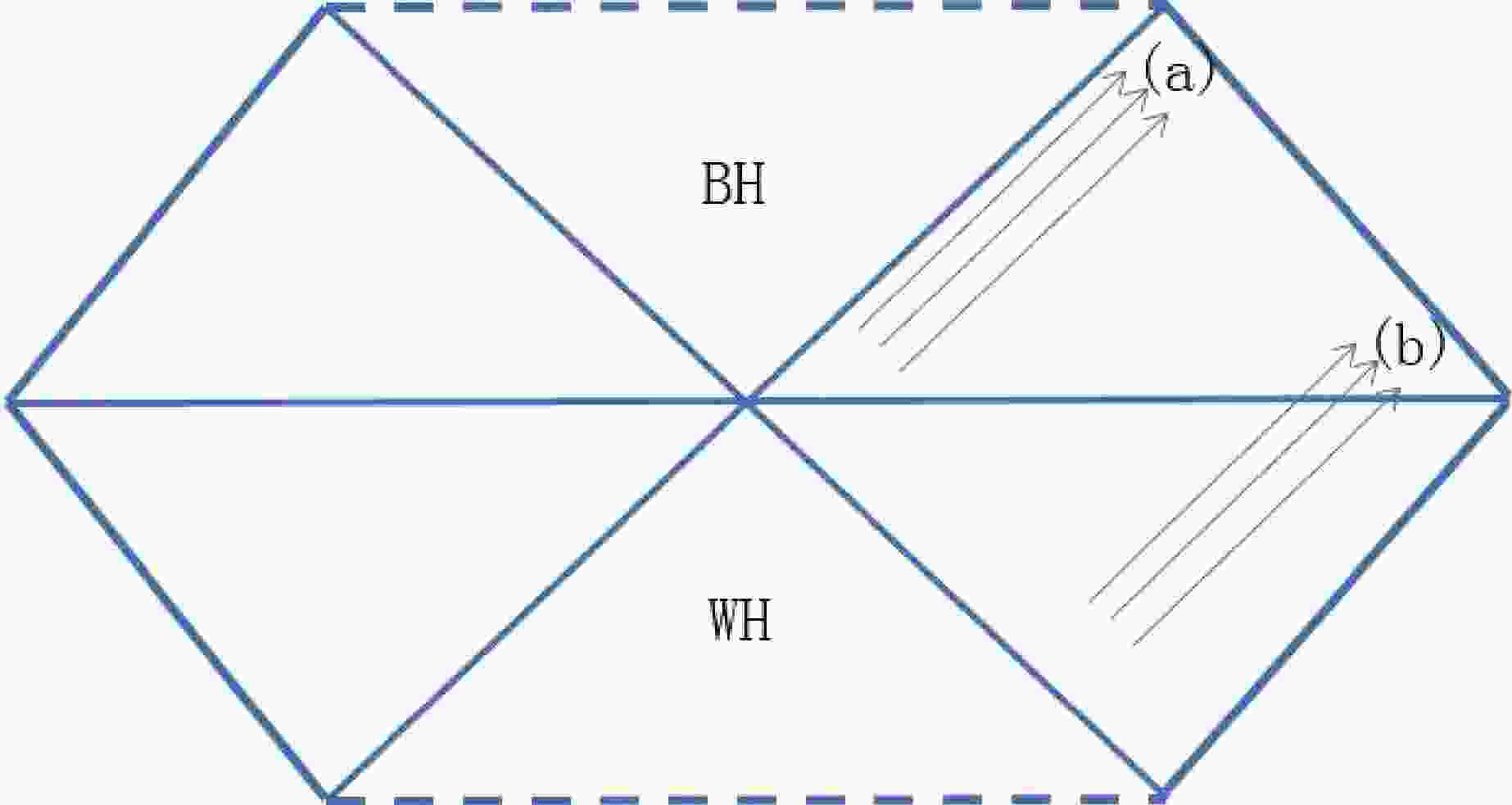
Figure 1 depicts white and black hole regions. We can easily see that any world line in the asymptotic region cannot be distinguished as belonging to the black or white hole. However, one question can be asked observationally. It is well known that an object exists at the center of our galaxy. Often, we refer it as a black hole corresponding to the black hole region in Fig. 1. However, it is not clear whether this black hole is formed by a star collapsing or it evolves from a white hole as depicted by Fig. 1. If it is formed by a star collapsing, the observer is located at relatively late point in the diagram, which corresponds to position (a) in the figure. In contrast, if it evolves from a white hole, the observer may be located at relatively early point, which corresponds to position (b) in the figure. An accretion disk is a common object around a strong gravitational object. This paper investigates the possibility of using accretion disk observation to distinguish a white hole (position (b)) from a black hole (position (a)).

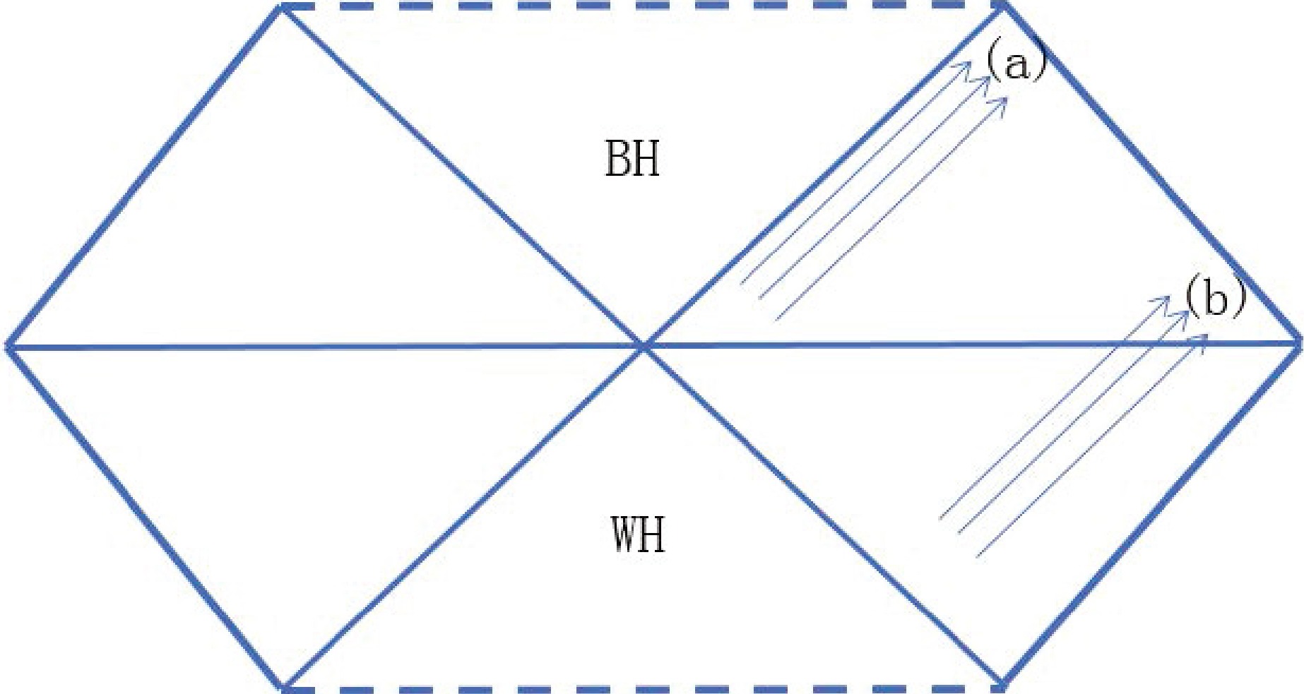
Figure 1.  (color online) Black hole (BH) and white hole (WH) corresponding to two different regions in a spacetime. If the observer is at position (a), the observation corresponds to a black hole. If the observer is at position (b), the observation corresponds to a white hole. The arrows indicate the signals of observation. Approximately, positions α and β in Fig. 6 of Ref. [7] respectively correspond to positions (a) and (b) here.

In Sec. II, we discuss the accretion disk structure around a white hole. In Sec. III, we analyze the properties of null geodesics around a white hole. Based on these results, we present the image of a white hole in Sec. IV. Both thin and thick disks are discussed. Finally, we summarize the paper in Sec. V. Throughout the paper, we use geodesic units with $ c = G = 1 $.

Because the white hole admits the same Schwarzschild metric as usual, the time-like geodesic equation has the same form as that in well-known literature such as [8−10]:

Here, τ is the proper time of the object moving along the given time-like geodesic. r and ϕ are Schwarzschild coordinates. M is the mass of the white or black hole. The specific angular momentum L and specific energy E are measured by an observer at infinity. U is the effective potential analogous to the one in Newtonian dynamics.

The orbits can be divided into four catalogs: (1) The generalization of the eccentric orbit of Newtonian dynamics. We still call them eccentric orbits. (2) The generalization of unbound orbit of Newtonian dynamics. We call them hyperbolic orbits for convenience. (3) Orbits that connect the original point ($ r = 0 $), or to say the singularity, and the infinity. (4) Bounded orbits that connect the original point. These orbit catalogs are determined by the parameters E and L and the orbit location. Fig. 2 shows the relation between the orbit catalog and the parameters. Three important lines in Fig. 2 divide the regions. The blue line corresponds to $ E^2 = 1 $, which is the asymptotic value of $ U^2 $ for $ r\rightarrow\infty $. The green and red lines correspond to the local minimal and maximal $ U^2 $, respectively, with respect to r.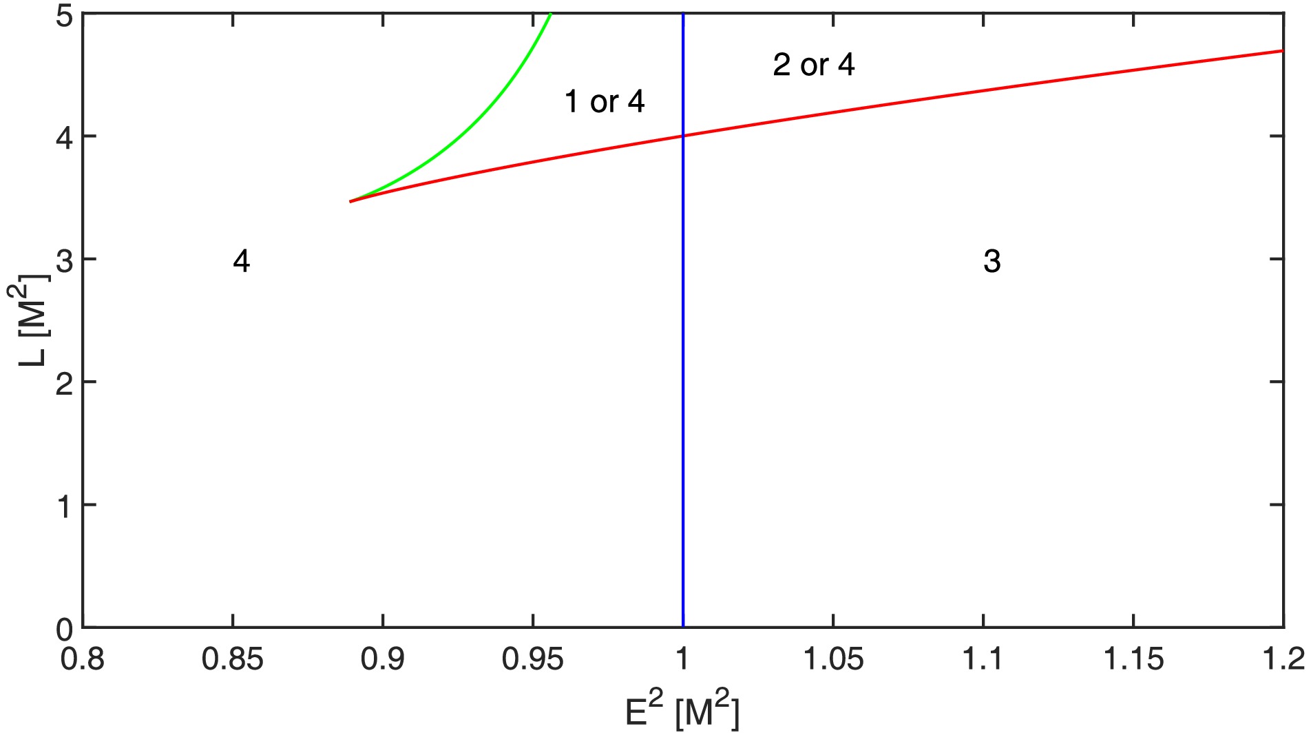

Figure 2.  (color online) Relation between the time-like geodesic orbit catalog and the parameters E and L. The number indicates the orbit catalog of the corresponding parameter region. The green and red lines correspond to $U^2_{{\rm{min}}}$ and $U^2_{{\rm{max}}}$, respectively.

The intersection point of the green and red lines is $ L = 2\sqrt{3}M $, and $ E^2 = \dfrac{8}{9} $. Analogous to Newtonian dynamics, we have $ U_{\rm{min}} = -\infty $ and $ U_{\rm{max}} = +\infty $. Additionally, the asymptotic value of U with respect to r is 0. Therefore, for Newtonian dynamics, we have only eccentric orbits (type 1) and hyperbolic orbits (type 2), which are divided simply by $ E = 0 $.

For black holes, objects moving along the third and fourth catalog orbits will finally reach the original point. In contrast, for white holes, objects moving along the third and fourth catalog orbit all begin from the original point. The third catalog orbits will let the objects escape to infinity.

For the fourth catalog orbits, the objects return to the original point, which corresponds to the singularity of the black hole that occurs at the later time of the white hole in question. For clarity, we call this black hole a post-black hole in this paper. Corresponding to Fig. 1, we plot world lines for the four catalog orbits in Fig. 3.

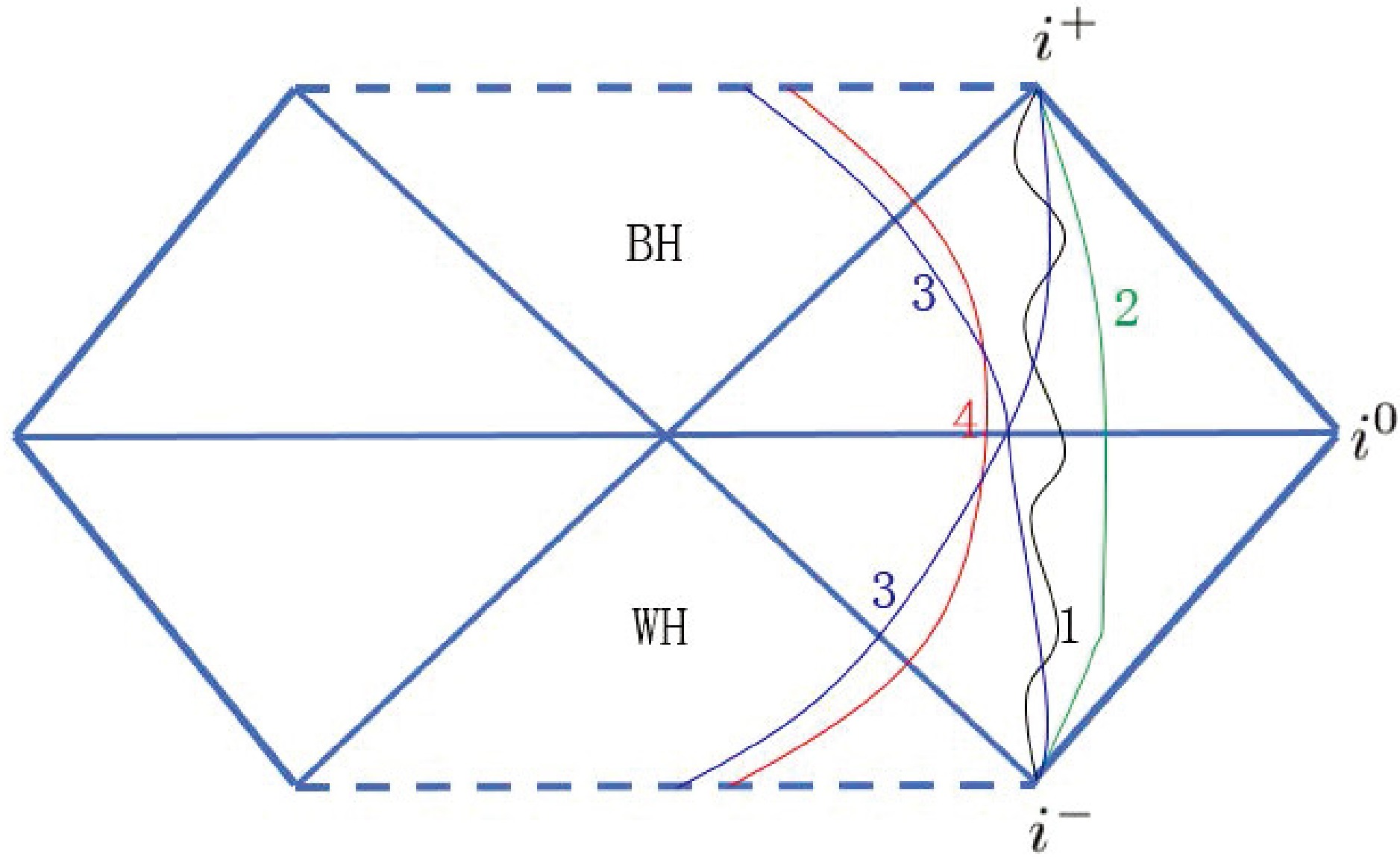
Figure 3.  (color online) Example world lines for the four catalogs orbits. $i^0$, $i^+$, and $i^-$ are used to indicate spatial, future time, and past time infinities, respectively.

Figure 3 shows that catalog (1) and (2) orbits, i.e., eccentric and hyperbolic orbits, respctively, are shared by the white and post-black holes. This behavior is consistent with the fact that eccentric and hyperbolic orbits are time reversible. The difference between catalog (1) and (2) orbits is that the r of (2) orbits extends to infinity when the orbit approaches $ i^{\pm} $, whereas that of (1) orbits remains bounded. The remaining two catalogs are different for black and white holes. For black holes, $ \dfrac{{\rm d}r}{{\rm d}\tau}\geq0 $, whereas for white holes, $ \dfrac{{\rm d}r}{{\rm d}\tau}\leq0 $.

When an object is moving around a black hole, certain dissipation effects will make the object orbit have a circular orbit that corresponds to the green line in Fig. 2. The object will then lose more energy and angular momentum. Corresponding to Fig. 2, the object will move along the green line to the intersection point of the green and red lines, which corresponds to the inner most stable circular orbit of a black hole. Subsequently, the orbit type converts to catalog 4. The object falls into the black hole. This conversion occurs at $ r = 6M $. If all of the objects appearing at the singularity of a white hole enter in this manner, they cannot escape farther than $ 6M $. Note that the black hole mentioned here differs from the aforementioned post-black hole with respect to the white hole in question. To distinguish them, we call this a pre-black hole. Consequently, as observers located far from the white hole, we do not expect to meet objects moving along catalog orbit (3) or (4). In other words, the picture that a white hole will spray a large number of objects is not true.

Based on the above analysis, we can conclude that the matter moving around a white hole can be divided into two classes. One class is matter positioned farther from the white hole. This matter must come from outside the white hole. The other class is matter located near the white hole. This matter may come from outside or inside the white hole. For the objects coming from inside the white hole, if they do not interact with those coming from outside, they will presently fall into the corresponding black hole. In contrast, if they interact strongly with the objects emerging from outside of white hole and their orbits change to catalog (1) and (2) orbits, they can remain in place for a long time. Thus, the matter constituting the accretion disk of a white hole must move along the eccentric or hyperbolic orbits. In other words, the structure of the accretion disk of a white hole is exactly the same as that of a black hole.

Again, because the white hole admits the same Schwarzschild metric as a Schwarzschild black hole, the null geodesic equation has the same form as a black hole [8]:

No proper time exists for null curves. Now, λ is any affine parameter for null geodesics. Similar to the time-like geodesic case discussed in the above section, B is the effective potential for null geodesics. Different from the time-like geodesics, B admits only a local maximal

The orbits can be divided into three catalogs. The first one (1) corresponds to orbits for light bending phenomena. The light originates from infinity (past null infinity $ {\cal{I}}^- $) and returns to infinity (future null infinity $ {\cal{I}}^+ $). The second catalog orbit (2) connects infinity and the original point, which may be the singular point of the black or white hole. The third catalog orbit (3) starts from the singularity of the white hole and end at the singularity of the black hole. We plot example world lines for these three catalog null geodesics in Fig. 4. We have $ E^2>B^2_{\rm{max}} $ for catalog (2) and $ E^2<B^2_{\rm{max}} $ for catalogs (1) and (3). The dividing scenario $ E^2 = B^2_{\rm{max}} $ corresponds to light ring that occurs at $ r = 3M $. This means that catalog (3) light is bounded in region $ r<3M $.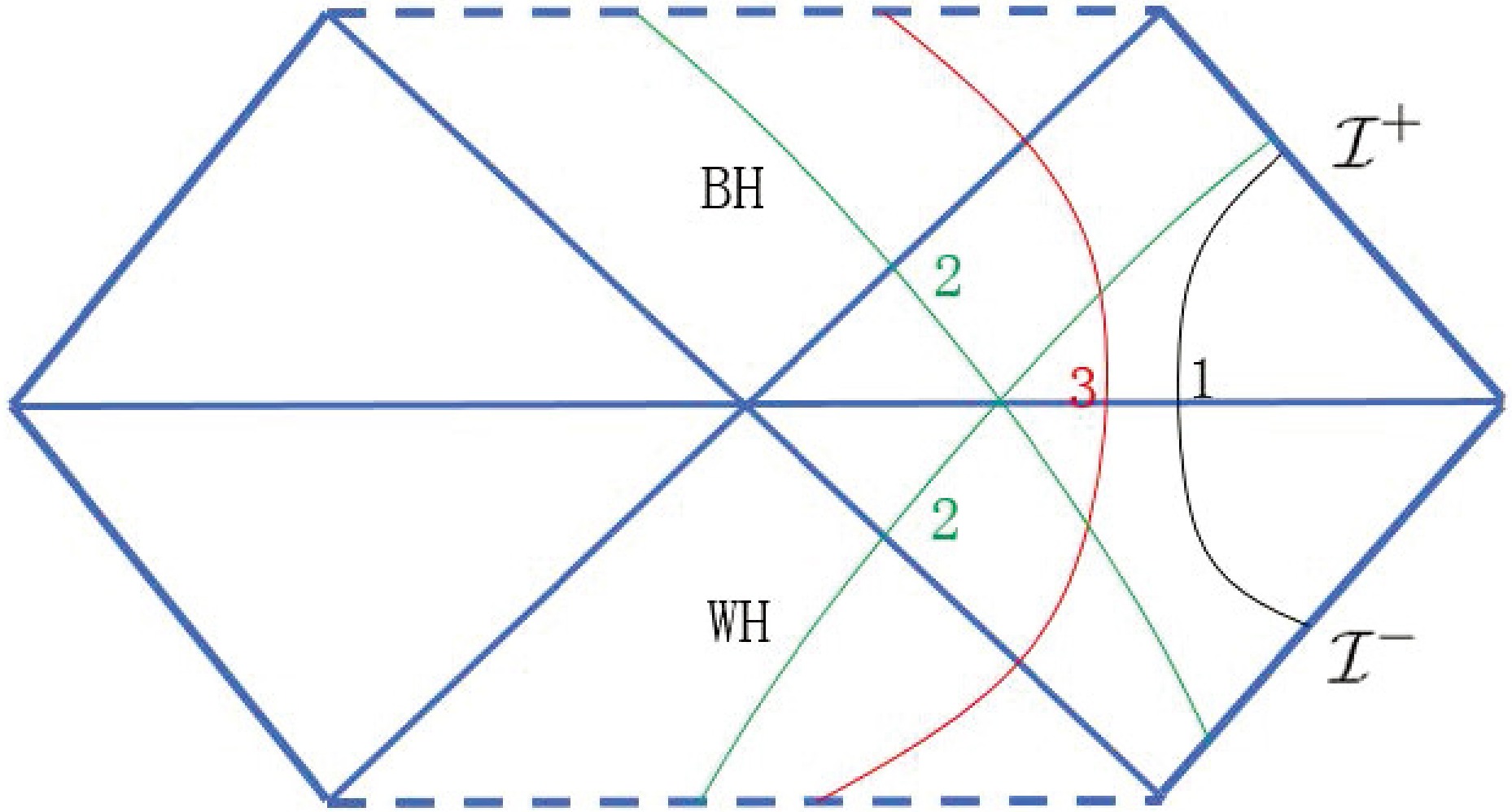

Figure 4.  (color online) Example world lines for the three catalog orbits of null geodesics. ${\cal{I}}^+$ and ${\cal{I}}^-$ indicate future and past null infinities, respectively.

Based on the above analysis, we can observe that as observers sitting far from the white hole, we can observe lights only belonging to catalogs (1) and (2). For the light of catalog (2), the source may be outside a white hole. Furthermore, we know that the structure of the accretion disk of a white hole is exactly the same as that of a black hole, which means that we cannot distinguish a white hole from a black one based on the image observation of the accretion disk if no light source exists inside the white hole.

We have observed from the above section that if no light comes from a white hole, the image of a white hole is exactly the same to that of a black one. In this section, we consider a scenario with light sources inside a white hole. No matter can remain in a white hole for a long time. Therefore, no light source can exist inside a white hole. However, any light falling into a black hole emerges from the corresponding white hole at a later time. Therefore, some light may possibly emerge from a white hole through the spacetime structure black hole-white hole conversion. A similar scenario has been discussed in [7, 11]. However, their discussions are for loop quantum or regular black hole metrics. In this paper, we are examining the behavior of standard white holes.

The image behavior strongly depends on the properties of the light source. If the light source is only the accretion disk outside of a white hole, its image is the same as a black hole [12]. If the light sources include both outside and inside ones, the image is simply the superposition of the sub-images affected by the outside and inside sources. Thus, in this section, we need only consider light sources inside a white hole. Such sources can only be outside of the corresponding black hole at an earlier time than the white hole in question. Note that this black hole is the pre-black hole with respect to the white one.

The light passing through the pre-black and white holes must belong to the catalog (2) orbit shown in Fig. 4. We can express the orbit solution explicitly as follows [8]. First, the impact parameter must fall in the range

Subsequently, the equation

admits one and only one real solution

We denote

With notations p and e, the orbit solution can be expressed as

where F is the first kind of the elliptic integral

and we introduce the notations

Furthermore, ψ is determined through

by ξ. Here, $ + $ corresponds to $ \xi>\hat\xi $, and $ - $ corresponds to $ \xi<\hat\xi $, with

Through relation (24), $ \psi_\infty $ corresponds to

and when $ \xi = \xi_0 $, we have $ \psi = 0 $. Here, r and ϕ are the Schwarzschild coordinates.

To compare the image behavior of white and black holes, we follow the same model problems as in [12]. First, we consider a white hole with its corresponding earlier black hole that is illuminated from behind by a planar screen that emits isotropically with uniform brightness. We assume that the screen is infinitely far away and infinite in extent.

The lights with impact parameter $ b<3\sqrt{3}M $ will fall into the black hole and emerge from the white hole in question. The orbit part outside the white hole is parity symmetric with respect to the original point to the part before the light falls into the black hole. We show an example in Fig. 5, which is based on solutions (16) and (18). The solid and dashed lines represent the parts moving in the black and white hole spacetime regions, respectively. Therefore, these lights return ideally uniform when they approach the observer. Consequently, we observe a uniform disk with radius $ 3\sqrt{3}M $ in the current case.

Figure 5.  Example trajectory of the catalog (2) orbit of the null geodesic. The solid and dashed lines represent the parts moving in the black and white hole spacetime regions, respectively. They are parity symmetric respect to the original point.

The observational appearance of a white hole with a backlit pre-black hole is shown in Fig. 6.

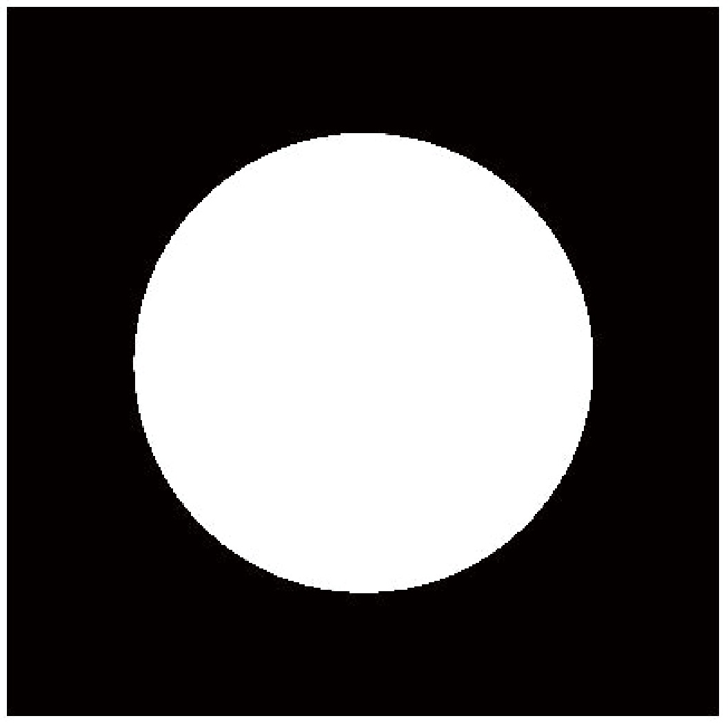
Figure 6.  Observational appearance of a Schwarzschild white hole with a pre-black hole that is backlit by a large distant screen of uniform isotropic emission. The brightness (white region) is uniform where it is nonzero. The bright region is a disk with a radius $3\sqrt{3}M$.

We consider a case viewed from a face-on orientation. We assume that the disk emits isotropically in the rest frame of static world lines. In this scenario, the specific intensity $ I_\nu $ of emission depends only on the radial coordinate:

where ν is the emission frequency in a static frame. Thus, the observed intensity can be expressed as

where $ r_n(b) $ is the radial coordinate of the nth source locating on the disk for the observer with impact parameter b. We solve $ r_n(b) $ using the following procedure. First, we denote

We denote the corresponding ψ of $ \phi_n $ through (18) as $ \psi_n $

Thus, we have

We denote the corresponding ξ of $ \psi_n $ through (24) as $ \xi_n $

where $ a_n,b_n $, and $ c_n $ denote the coefficients of equation (33):

and $ \psi_0 $ corresponds to $ \xi = 0 $ through relation (24).

The resulting $ r_{1,2,3}(b) $ corresponds to the $ b<3\sqrt{3} $ part of Fig. 4 in Ref. [12]. Specifically, we have

In other words, if the inner edge of the accretion disk of the pre-black hole is farther than $ 4.3M $, no light is emerging from the white hole. For the case when the inner edge of the accretion disk of the pre-black hole is less than $ 4.3M $, in Fig. 7 we show two examples of the white hole image with an optically and geometrically thin pre-black hole disk emission. Equations (38)−(40) indicate that the white hole image is at most a ring band $ (2.85M,3\sqrt{3}M) $. Owing to the redshift and superposition effects as shown in (29), the out boundary of the ring band is much brighter. Both examples in Fig. 7 are consistent with this theoretical prediction. Otherbehaviors of the image depend on the emission density profile.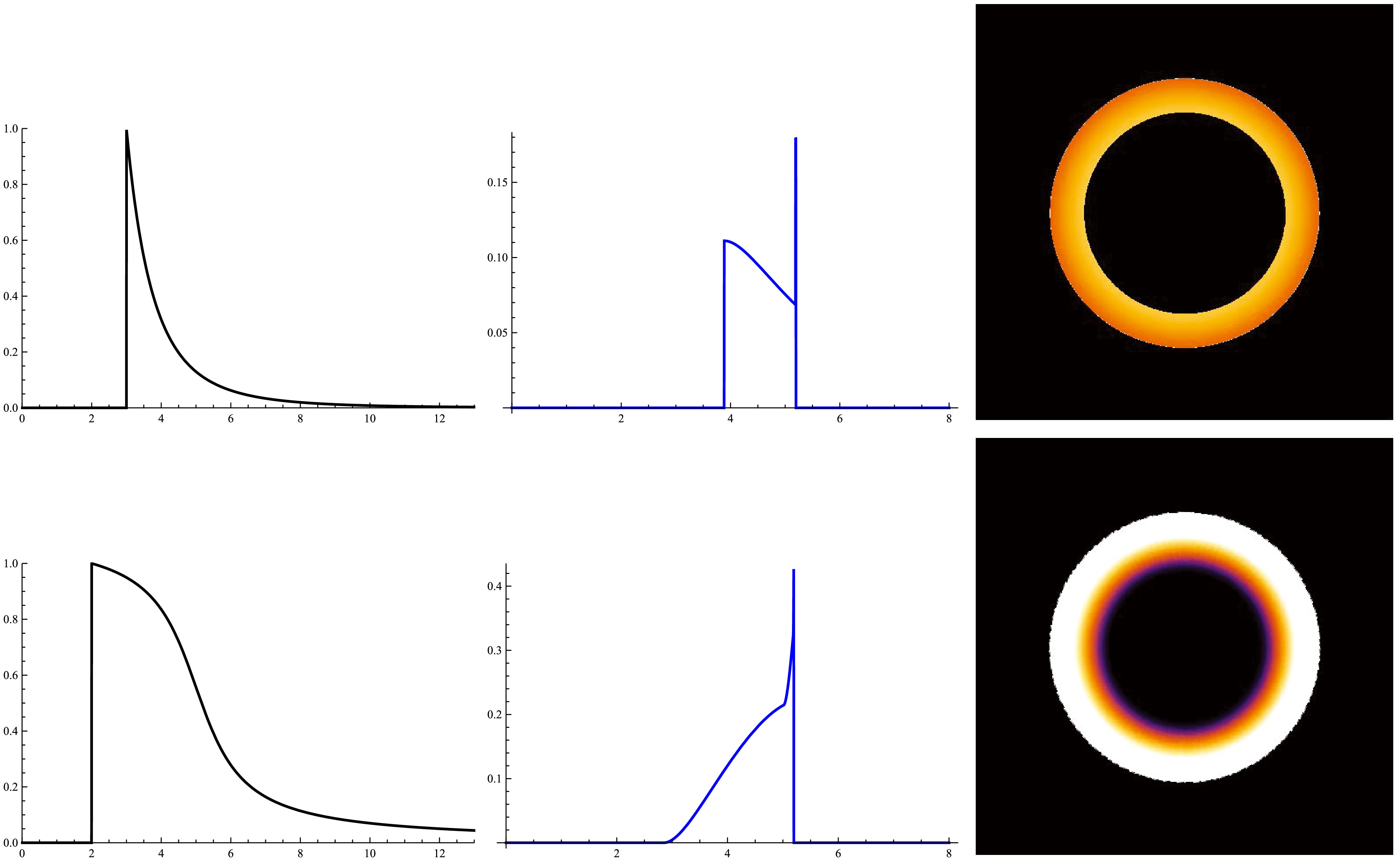

Figure 7.  (color online) The two rows correspond to two examples of the white hole image with an optically and geometrically thin pre-black hole disk emission. The left column corresponds to the emission density profile of the disk $I(r)$. The middle column corresponds to the observed density profile $I^{ {\rm{obs}}}(b)$. The right column corresponds to the observational appearance viewed from a face-on orientation. Here, the densities have been normalized to the maximum value $I_0$ of the emitted intensity outside the horizon of the pre-black hole.

We follow [12] to assume that the disk admits a uniform emissivity. Thus, the observed density can be expressed as

where the factor $ \left(1-\dfrac{2M}{r}\right)^2 $ is the redshift effect, and $ \left(1-\dfrac{2M}{r}\right)^{-1} $ is the proper length effect of the Schwarzschild metric. These two effects were neglected in [12]. The optical path of the light ray may intersect with the disk several times. Along with the orbit, we denote the start and end points of the nth intersection as $ P_{n0} $ and $ P_{n1} $, respctively. Substituting the related null orbit solution, we obtain

where $ {}' $ is the derivative with respect to the orbit parameter ξ, and $ \xi_{n0} $ and $ \xi_{n1} $ correspond to the orbit parameter of points $ P_{n0} $ and $ P_{n1} $, respctively. Here, we denote the proportional constant as $ I^h $. Regarding the related null orbit, we obtain

Corresponding to Fig. 6 of [12], we also investigate three types of geometrically thick disks: rectangular, wedge-shaped, and spherical. We plot the results in Figs. 8−10. For the rectangular ones, the result becomes the result of the thin disk discussed in the above section when the thickness decreases. In any case, the ring at $b = 3\sqrt{3}M$ is the brightest.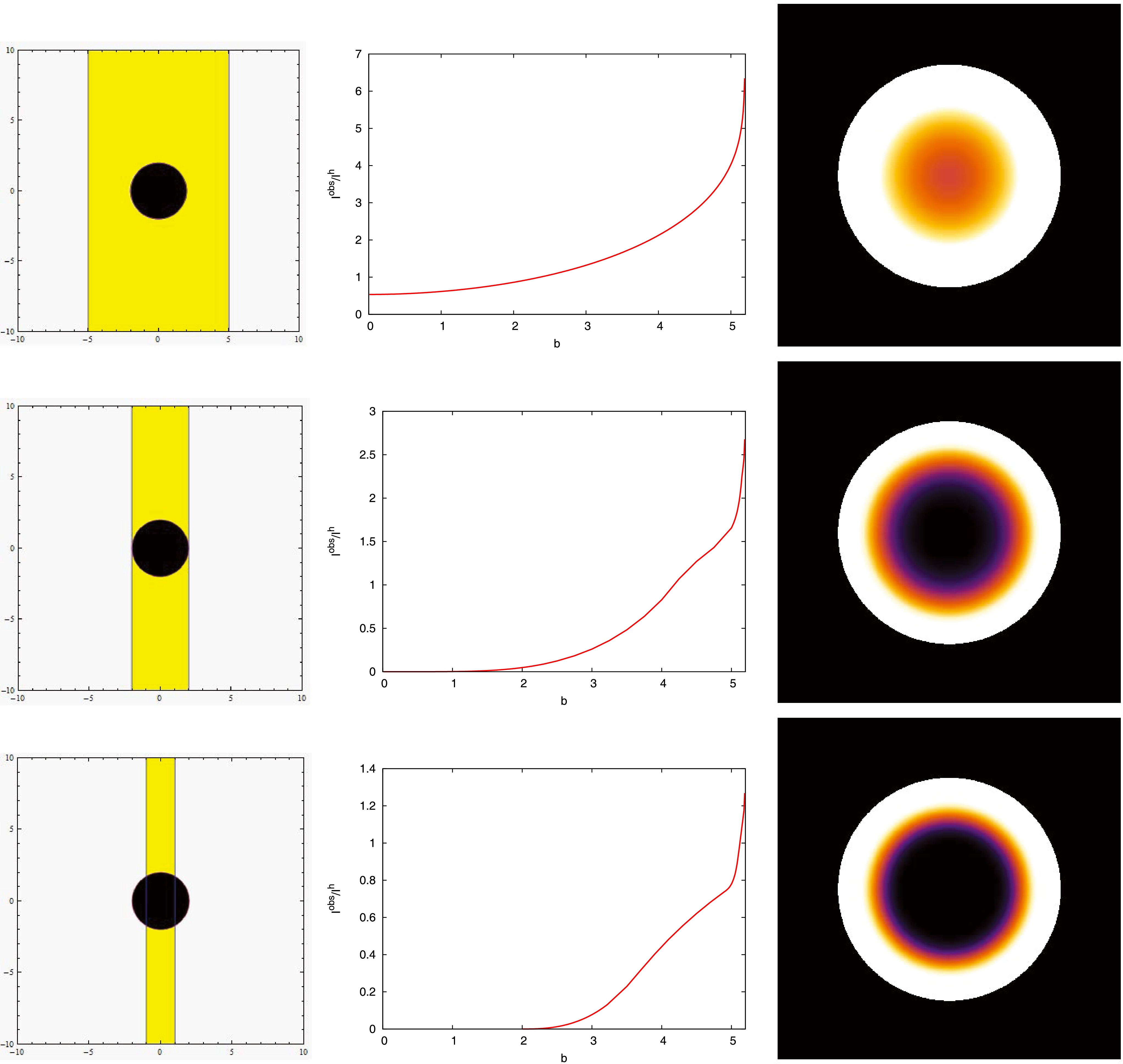

Figure 8.  (color online) The three rows correspond to three examples of the white hole image with a rectangular geometrically thick pre-black hole disk (yellow region) emission. The left column corresponds to the profile of the disk. The middle column corresponds to the observed density profile $I^{ {\rm{obs}}}(b)$. The right column corresponds to the observational appearance, viewed from a face-on orientation. Here, the densities have been normalized to the proportional constant $I^h$.

Figure 9.  (color online) The same as Fig. 8 but for wedge-shaped geometrically thick pre-black hole disk emission.

Figure 10.  (color online) The same as Fig. 8 but for spherical geometrically thick pre-black hole disk emission.

Different from the scenario in [12], the red-shift factor $ \left(1-\dfrac{2M}{r}\right)^2 $ and proper length factor $ \left(1-\dfrac{2M}{r}\right)^{-1} $ involved in (42) cannot be neglected. Using the example shown in the top row of Fig. 8, we show the results when the proper length factor $ \left(1-\dfrac{2M}{r}\right)^{-1} $ is neglected and both the red-shift factor $ \left(1-\dfrac{2M}{r}\right)^2 $ and proper length factor $ \left(1-\dfrac{2M}{r}\right)^{-1} $ are neglected in Fig. 11. The figure shows that the effects of the red-shift factor $ \left(1-\dfrac{2M}{r}\right)^2 $ and proper length factor $ \left(1-\dfrac{2M}{r}\right)^{-1} $ are significant. Accordingly, we only show full results in Figs. 8−10 without any approximation.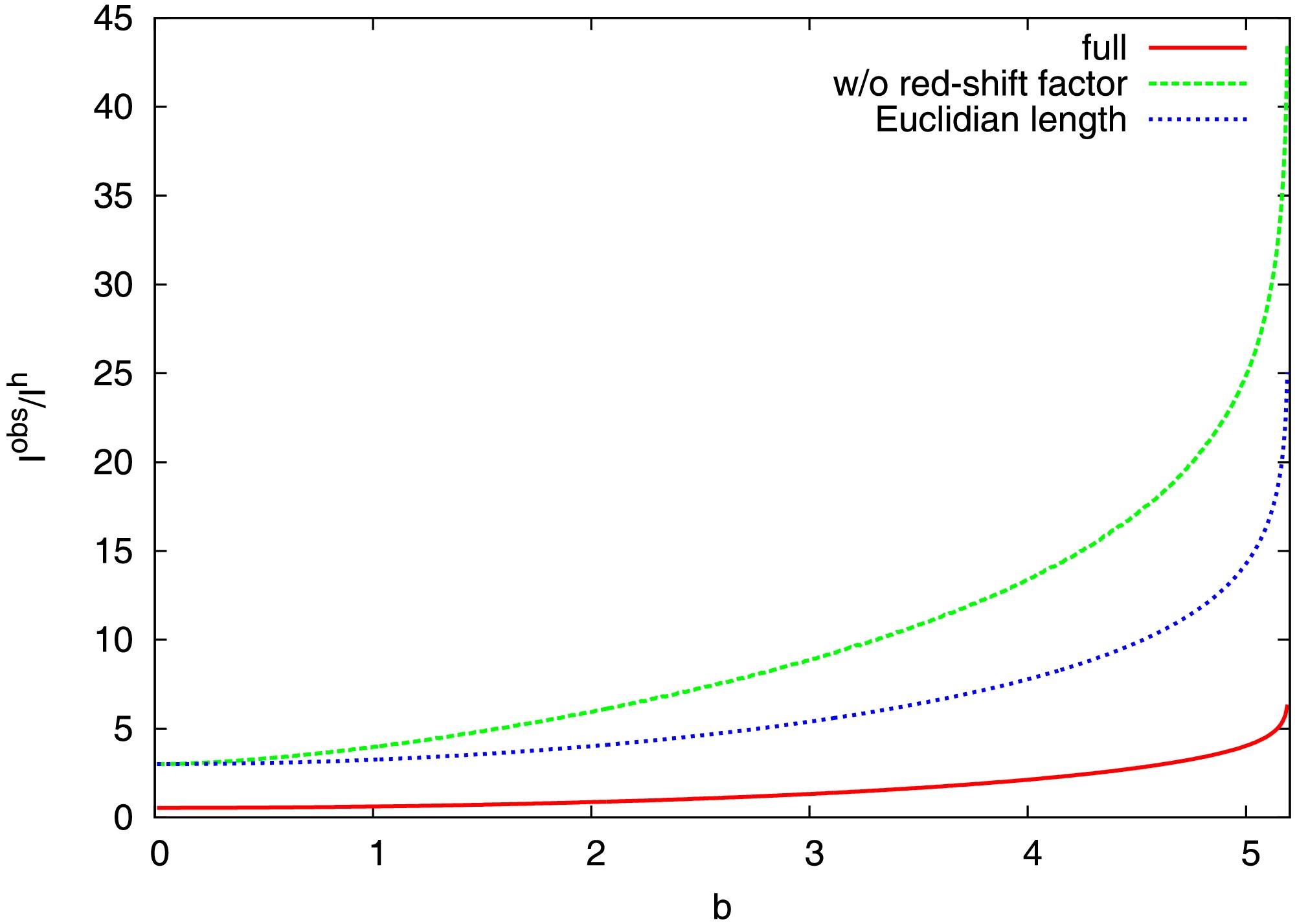

Figure 11.  (color online) Effect comparison of the red-shift factor $\left(1-\dfrac{2M}{r}\right)^2$ and proper length factor $\left(1-\dfrac{2M}{r}\right)^{-1}$ involved in (42). The line marked with “full” means the result closely following (42). The line marked with “w/o red-shift factor” means replacing the red-shift factor $\left(1-\dfrac{2M}{r}\right)^2$ with 1. The line marked with “Euclidian length” means replacing the red-shift factor $\left(1-\dfrac{2M}{r}\right)^2$ with 1 and replacing the proper length factor $\left(1-\dfrac{2M}{r}\right)^{-1}$ with 1. The disk profile corresponding to the top row of Fig. 8 is used in this plot.

In the standard general relativity theory, white and black holes admit the same metric form. A white hole is simply a spacetime region that is earlier than the corresponding black hole spacetime region. If a black hole is formed through a star collapsing, the white hole spacetime region is replaced by a star inner solution. Therefore, white holes do not exist for such cases. If all black holes formed in this manner, we can believe that white holes do not exist in our universe.

Recent research results indicate that quantum gravity effect may cause black holes to convert to white ones. In other words, if quantum gravity theory is true, white holes should exist. This theoretical prediction provides us a challenge: Can we confirm whether white holes exist in our universe? Whether the answer is yes or no, it can provide important information for quantum gravity theory.

Assuming that the quantum gravity effect appears only in a limited region, we use standard general relativity to perform observational analysis in this paper. We observe that the disk structure around a white hole is exactly the same as that around a black hole. Thus, if no light emeerges from the white hole, we can not distinguish a white hole from a black one.

One possibility to recognize a white hole is light sources located outside of a pre-black hole. We have investigated white hole images for several simplified disks around a pre-black hole. According to our results, if the image is strictly smaller than the light ring region of the object, we can deduce that it is a white hole. Furthermore, we are certain that the accretion disk does not occur outside the white hole; instead, it is outside the pre-black hole.

The light ring of M87 corresponds to about 20 μas. The observation presents rings with radius about 42 μas [13] and 64 μas [14], which are significantly larger than 20 μas. Based on these observation results, we are certain that M87 is not a white hole with a pre-black hole accretion disk. Hoever, we cannot distinguish it is a white hole with an accretion disk and jet or a black hole with an accretion disk and jet.

The light ring of Sgr A$ {}^* $ corresponds to about 27 μas. The observation presents rings with a radius of about 52 μas [15], which is also significantly larger than 27 μas. Therefore, we are currently uncertain that Sgr A$ {}^* $ is a black or white hole.

In summary, we currently cannot certainly confirm if white holes exist. More observations and theoretical investigations to distinguish a white hole from a black hole are required.