Critical collapse in asymptotically anti-de Sitter spacetime

Gravitational collapse is a basic process in astrophysics, which describes the continuous shrinkage of a star under its own gravity. This phenomenon is crucial for understanding the structural formation of our universe. Since the pioneering work of Oppenheimer and Snyder on uniform-density dust collapse [1], research in this field has advanced significantly, revealing complex dynamics in various astrophysical scenarios.

The outcome of gravitational collapse depends critically on the initial density of matter. Matter with sufficient density will form a black hole, while matter below this threshold will disperse to infinity. Choptuik's numerical simulation of the collapse of a spherically symmetric massless scalar field reveals a phenomenon known as critical collapse, which occurs near the threshold of black hole formation [2]. Above this threshold, a small black hole forms. The black hole mass follows the power-law relation $M_{\rm BH} \propto (p-p^{*})^{\gamma}$, where $M_{\rm BBH}$ is the black hole mass on formation, p is a parameter from a family of initial data, $ p^{*} $ is the critical value, and $ \gamma \approx 0.37 $ is a universal constant independent of initial conditions. Choptuik further observed that, near critical evolutions, the scalar field asymptotically approaches a discretely self-similar form, characterized by an echoing period of $ \Delta \approx 3.44 $.

Brady et al. [3] investigated critical behavior in the collapse of a massive scalar field and identified two distinct types of phase transitions: Type I collapse occurs when the characteristic scale is larger than $ 1/m $, and Type II collapse occurs when the characteristic scale is smaller than $ 1/m $, where m is the mass parameter. Hirschmann and Eardley [4] explored the critical collapse of a massless complex scalar field and determined that the critical exponent is $ \gamma \approx 0.38 $, which is consistent with the findings in Ref. [2]. Jiménez-Vázquez and Alcubierre investigated the critical collapse of a massive complex scalar field and identified two types of critical collapse [5]; Type I collapse features an unstable boson star in the ground state as the critical solution, while Type II collapse has results similar to those in Choptuik's study [2]. Our work focuses exclusively on Type II critical phenomena.

Further research has explored the collapse of various types of matter, including scalar field [6−10], fluid [11−18], and Yang-Mills field [19−24]. There have also been numerous investigations on gravitational collapse in modified gravity models [25−30]. Recently, significant research has been conducted on axisymmetric cases [31−34]. For reviews on gravitational collapse, see Refs. [35, 36].

Numerical simulations by Bizoń and Rostworowski demonstrated that, in anti-de Sitter (AdS) spacetime, even arbitrarily small initial data can result in black hole formation [37]. Large initial data directly lead to black hole formation, while small initial data can form a black hole after multiple reflections at the outer boundary. Further discussions on the AdS instability conjecture can be found in Refs. [38−48].

Vera investigated the critical collapse of a massless scalar field in asymptotically flat and asymptotically AdS spacetimes [49]. He focused solely on the initial collapse without accounting for the influence of the outer boundary. Through fine-tuning of the initial scalar field amplitude, he presented the following relationship between the critical amplitude $ A^{*} $ and AdS radius L:

where $ A^{*}_{\infty} $ is the critical amplitude in asymptotically flat spacetime. The undetermined function f depends on L and possibly on the center ($ v_{0} $) and width ($ \sigma $) of the initial scalar field. In our previous study [50], we found that the critical amplitude $ A^{*} $ for the first collapse of a massless scalar field in asymptotically AdS spacetime exhibits a linear relationship with the cosmological constant $ \Lambda $. This relationship is also influenced by the initial scalar field's width and position. In this paper, we further investigate whether this linear relationship between the critical amplitude $ A^{*} $ and cosmological constant $ \Lambda $ holds for a real scalar field with a potential and a massive complex scalar field. Additionally, we explore the effect of the scalar field's coupling constants on the critical amplitude.

The remainder of this paper is organized as follows. Section II outlines our methodology for simulating the collapse of real and complex scalar fields with potentials in asymptotically AdS spacetime. Sections III and IV present our findings on the behavior of the critical amplitude in real and complex scalar fields, respectively. The results are summarized in Sec. V. Throughout this paper, we set $ c=1 $ and $ G=1 $.

Firstly, we consider the collapse of a real scalar field $ \phi $ with a potential in asymptotically AdS spacetime. The action for this system is

where R represents the Ricci scalar, $ \Lambda $ denotes the cosmological constant, and $ V(\phi) $ is the potential term for the scalar field. We obtain the equations of motion by varying the action with respect to the metric and scalar field:

where the prime symbol denotes the derivative with respect to $ \phi $, and $ T_{\mu\nu} $ is the energy-momentum tensor for the scalar field

We perform simulations in double-null coordinates,

For convenience, we introduce $ \Lambda=-3/L^{2} $, where L represents the AdS radius. Then, the Einstein equations can be expressed as follows:

where $ (_{,u}) $ and $ (_{,v}) $ denote the partial derivatives with respect to u and v, respectively. The equation of motion for the scalar field is

Following Hamade's method [51], we introduce the following:

Using these variables, we rewrite Eqs. (6)−(10) as follows:

The initial values for d and q are

where A, $ \sigma $, and $ v_{0} $ represent the initial amplitude, width, and position of the scalar field, respectively. Boundary conditions are set at the $ u=v $ axis. On this axis, we apply $ r=0 $, $ f=-g $, $ a=2g $, $ p=q $, $ a_{,r}=0 $, and $ s_{,r}=0 $. For the asymptotically flat case, we simply set the initial condition of d and all L-related terms to zero.

Additionally, the definition of Hawking mass is

We also introduce the proper time T on the $ u=v $ axis as

In numerical simulations, we use a fourth-order Runge-Kutta method to integrate Eqs. (11), (13), (14), and (18), while employing a predictor-corrector algorithm to evolve Eqs. (17) and (19). Details on the simulation can be found in Refs. [49, 51, 52].

For all simulations presented in this paper, we employ $ 10^{4} $ grid points and a $ 10^{-3} $ interval in the spatial direction. Since we are only studying the critical amplitude behavior during the first collapse, it is necessary to place the timelike boundary of AdS spacetime outside our computational domain [49]. Therefore, we choose AdS spacetime radii of $L=4,\,5,\,6,\,8,\,10,\,20,\,40,\,100,\,200,\,\infty$. In our simulations, black hole formation is considered when $ g < 10^{-4} $, at which point the program terminates. We fix other parameters and use the bisection method to determine the critical amplitude $ A^{*} $ to 12 significant figures.

The action describing the collapse of a massive complex scalar field $ \Phi $ is

where $\Phi=\phi_{R}+{\rm i}\phi_{I}$ is a complex scalar field, and $ \Phi^{*} $ is its complex conjugate. The equations of motion are obtained by varying the action with respect to the metric and scalar field:

where the energy-momentum tensor $ T_{\mu\nu} $ for the complex scalar field is

In double-null coordinates, the equations of motion are

We introduce the auxiliary variables $ s_{1} $, $ p_{1} $, $ q_{1} $, $ s_{2} $, $ p_{2} $, $ q_{2} $, c, d, f, and g as follows:

Then, Eqs. (28)−(33) can be expressed as follows:

We set the initial conditions for d, $ q_{1} $, and $ q_{2} $ as

On the axis of $ u=v $, we set $ r=0 $, $ f=-g $, $ a=2g $, $ p_{1}=q_{1} $, $ p_{2}=q_{2} $, $ a_{,r}=0 $, $ s_{1,r}=0 $, and $ s_{2,r}=0 $. In the asymptotically flat spacetime, terms related to L and the initial condition of d are set to zero, while the setup of other parts remains unchanged. Our numerical algorithm follows the same approach as used in the real scalar field case.

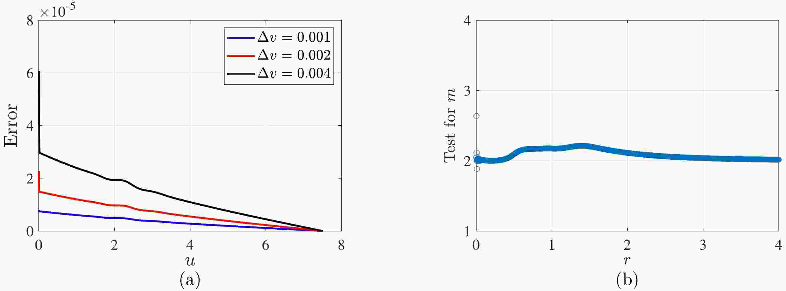
We describe the collapse of a massive real scalar field by numerically evolving Eqs. (12)−(19) with $V(\phi)= m_{1}^{2}\phi^{2}/2$. We first use Eq. (15) to verify the error at $ v=7.5 $ as it evolves over time. Figure 1 (a) shows the time evolution of the error for three different spatial grids. It is evident that as the grid spacing decreases, the error also decreases. We estimate the convergence order of the mass using $ \dfrac{m_{2N}-m_{N}}{m_{4N}-m_{2N}}=2^{n}+O(1/N) $, where m denotes the mass, N represents the number of spatial grid points, and n is the convergence order. Using $ N=2500 $, we obtain a convergence order of 2, as shown in Fig. 1 (b). Fixing $ \sigma^{2}=1/2 $ and $ v_{0}=2 $ in Eq. (21), we determine the critical amplitude $ A^{*} $ using the bisection method for different $ m_{1} $ and $ \Lambda $.

Figure 1.  (color online) Validation of code effectiveness for the initial profile parameters in Eqs. (15) and (21): $V(\phi)=\phi^{2}/2$, $ A=0.001 $, $ \sigma^{2}=1/2 $, $ v_{0}=2 $, and $ L=8 $. (a) Constraint of Eq. (15) as a function of u for $ v=7.5 $ under different spatial grid spacings. (b) Convergence order of $ m_{H} $ after 100 steps of u-evolution.

Figure 2 (a) shows the relationship between the scalar field s along the $ u=v $ axis with respect to $ \ln(T^{*}-T) $, where $ T^{*} $ denotes the time when the naked singularity forms. Combined with Table 1, we see that the echoing periods are almost the same, with $ \Delta\approx3.4 $, and exhibit slight relative displacements across different $ m_{1} $. Figure 2 (b) illustrates the power-law behavior of the black hole mass, with a slope of $ \gamma \approx 0.37 $. We also verified different L and $ m_{1} $, finding that $ \Delta \approx 3.4 $ and $ \gamma \approx 0.37 $. The value of $ \Lambda $ cannot be smaller because we must position the scalar field within the outer boundary of the AdS. Increasing the coupling parameter further would cause the program to break down.

Figure 2.  (color online) Scalar field behavior with potential $ V(\phi)=(1/2)m_{1}^{2}\phi^{2} $ in asymptotically flat spacetime. (a) Evolution of scalar field s ($ s=\sqrt{4\pi}\phi $) along $ u=v $ ($ r=0 $) axis. (b) Power-law behavior of the black hole mass in supercritical collapse. The initial profile parameters in Eq. (21) are $ \sigma^{2}=1/2 $, $ v_{0}=2 $. Specific values can be found in Table 1.

$ m_{1}^{2} $	$ A^{*} $	$ \Delta $	$ \gamma $
0	0.0513514784048	3.434	0.3796
1	0.0511273277151	3.472	0.3802
2	0.0509468015282	3.506	0.3674

Table 1.  Critical amplitude $ A^{*} $ (second column), echoing period $ \Delta $ (third column), and critical exponent $ \gamma $ (fourth column) of real scalar fields with potential $V(\phi)=m_{1}^{2}\phi^{2}/2$ in asymptotically flat spacetime. The initial profile parameters in Eq. (21) are $ \sigma^{2}=1/2 $, $ v_{0}=2 $. Critical amplitude is given to twelve significant figures, while echoing period and critical exponent are given to four significant figures.

Vera presented the following relationship of $ A^{*} $ as a function of L [49] (as shown in Fig. 3):

Figure 3.  (color online) Critical amplitude $ A^{*} $ in the initial scalar profile of Eq. (21) vs. AdS radius L (Fig. 5.17 in Ref. [49]).

where $ A^{*}_{\infty} $ is the critical amplitude in asymptotically flat spacetime, and $ f(L,v_{0},\sigma) $ is an undetermined function of L, potentially depending on $ v_{0} $ and $ \sigma $. However, we find that $ A^{*} $ has a simple relation with $ \Lambda $ ($ \Lambda=-3/L^{2} $) for fixed $ m_{1} $ (Fig. 4 (a)) as follows:

Figure 4.  (color online) Relations among the critical amplitude $ A^{*} $ of the initial scalar field with potential $V(\phi)=m_{1}^{2}\phi^{2}/2$, cosmological constant $ \Lambda $, and $ m_{1}^{2} $. (a) $ A^{*} $ vs. $ \Lambda $. The initial profile parameters in Eq. (21) are $ \sigma^{2}=1/2 $, $ v_{0}=2 $. (b) $ k_{\text{mass}} $ vs. $ m_{1}^{2} $.

where $ k_{\text{mass}} $ is the slope. Moreover, we find that $ k_{\text{mass}} $ varies linearly with respect to $ m_{1}^{2} $

as shown in Fig. 4 (b). Combining Eqs. (49) and (50), we obtain

We extend our research to the critical collapse of a real scalar field with potential $V(\phi)=\lambda\phi^{4}/4$. We first examine the errors at different spatial grid spacings, as shown in Fig. 5 (a), similar to the approach used in the massive scalar case. Using the same formula and setting $ N=2500 $, we determine that the convergence order of the mass, as shown in Fig. 5 (b), is also second order. We fix $ \sigma^{2}=1/2 $ and $ v_{0}=2 $ while varying $ \lambda $ and L to determine the critical amplitude $ A^{*} $. We consistently observe an echoing period of $ \Delta \approx 3.4 $ and critical exponent of $ \gamma \approx 0.37 $ in all configurations.

Figure 5.  (color online) Validation of code effectiveness for the initial profile parameters in Eqs. (15) and (21): $ V(\phi)=(0.3)\phi^{4} $, $ A=0.001 $, $ \sigma^{2}=1/2 $, $ v_{0}=2 $, and $ L=8 $. (a) Constraint of Eq. (15) as a function of u for $ v=7.5 $ under different spatial grid spacings. (b) Convergence order of $ m_{H} $ after 100 steps of u-evolution.

For a fixed $ \lambda $, we find that the critical amplitude $ A^{*} $ varies linearly with $ \Lambda $ (as shown in Fig. 6 (a)):

Figure 6.  (color online) Relations among the critical amplitude $ A^{*} $ of the initial scalar field with potential $V(\phi)=\lambda\phi^{4}/4$, cosmological constant $ \Lambda $, and $ \lambda $. (a) $ A^{*} $ vs. $ \Lambda $. The initial profile parameters in Eq. (21) are $ \sigma^{2}=1/2 $, $ v_{0}=2 $. (b) $ k_{\text{self}} $ vs. $ \lambda $.

Furthermore, as shown in Fig. 6 (b), we observe a linear relationship between the slope $ k_{\text{self}} $ and $ \lambda $

Although the slope increases with $ \lambda $, the rate of change is significantly smaller than that of the massive real scalar field. Combining Eqs. (52) and (53), we obtain

We are investigating the collapse of a massive complex scalar field in asymptotically AdS spacetime, using the method described above. As in the case of the real scalar field, we first verify the validity of the code. In Fig. 7 (a), we show the error in the constraint of Eq. (38) for different spatial grid spacings. Using the same grid size of $ N=2500 $ as in the real scalar field case, we find that the convergence order of the mass is approximately 2. The final results are presented in Fig. 7 (b). We obtain an echoing period and critical exponent consistent with those in [2]. By fixing $ m_{2} $ and varying L, we obtain a linear relationship between $ A_{1}^{*} $ and $ \Lambda $

Figure 7.  (color online) Validation of code effectiveness for the initial profile parameters in Eqs. (38), (46), and (47): $ V(\phi)=\Phi\Phi^{*} $, $ A_{1}=0.001 $, $ \sigma_{1}^{2}=1/2 $, $ v_{10}=2 $, $ A_{2}=0.001 $, $ \sigma_{2}^{2}=1/2 $, $ v_{20}=3 $, and $ L=8 $. (a) Constraint of Eq. (38) as a function of u for $ v=7.5 $ under different spatial grid spacings. (b) Convergence order of m after 100 steps of u-evolution.

As shown in Fig. 8 (a), this linear relationship holds for different $ m_{2} $. There is a linear relationship between $ k_{\text{complex}} $ and $ m_{2}^{2} $

Figure 8.  (color online) Relations among the critical amplitude $ A_{1}^{*} $ of the initial scalar field with potential $ V(\phi)=m_{2}^{2}\Phi\Phi^{*} $, cosmological constant $ \Lambda $, and $ m_{2}^{2} $. (a) $ A_{1}^{*} $ vs. $ \Lambda $. The initial profile parameters in Eqs. (46) and (47) are $ \sigma_{1}^{2}=1/2 $, $ v_{10}=2 $, $ A_{2}=0.01 $, $ \sigma_{2}^{2}=1/2 $, and $ v_{20}=3 $. (b) $ k_{\text{complex}} $ vs. $ m_{2}^{2} $.

as shown in Fig. 8 (b). This slope varies more rapidly than that observed in the massive real scalar field. Combining Eqs. (55) and (56), we obtain

Here, we need to clarify that, in asymptotically flat spacetime, the critical amplitude of the complex scalar field is significantly different from that of the real scalar field because the initial data setup for the massless scalar field is the same in both real scalar field models in this spacetime. However, the presence of the imaginary part in the complex scalar field introduces an additional energy contribution compared to the real scalar field, resulting in a critical amplitude that is notably smaller than that of the real scalar field.

Our numerical investigation of Type II critical collapse of real and complex scalar fields with potentials in asymptotically AdS spacetime revealed two main findings. Firstly, we observed echoing periods and critical exponents consistent with Choptuik's results across all configurations. Secondly, we found that for both real and complex scalar fields with potentials, the critical amplitude $ A^{*} $ of the initial scalar field exhibits a linear relationship with the cosmological constant $ \Lambda $. Specifically, for massive real scalar fields, the slope $ k_{\text{mass}} $ shows a linear dependence on the square of the real scalar field's mass $ m_{1}^{2} $. In the case of real scalar fields with quartic self-interaction, the slope $ k_{\text{self}} $ is linearly related to the coupling constant $ \lambda $. Similarly, for massive complex scalar fields, the slope $ k_{\text{complex}} $ correlates linearly with the square of the complex scalar field's mass $ m_{2}^{2} $. Therefore, we discovered that, across different matter fields, the critical amplitude exhibits a consistent linear relationship with the cosmological constant, and this slope is linearly correlated with the coupling strength of the scalar field potential.

These results significantly enhance our understanding of critical collapse phenomena. They not only elucidate the role of AdS geometry in critical collapse but also provide valuable insights into the intricate dynamics of gravitational systems near criticality. Our findings pave the way for further exploration of the rich phenomenology of critical behavior in curved spacetimes.