Black holes in general relativity coupled with nonlinear electrodynamics surrounded by perfect fluid dark matter: Thermodynamics, particle motion, and black hole shadow

Black holes are among the most challenging and debated aspects of Einstein's theory of relativity. Regular or non-singular black holes have been predicted using certain energy-momentum tensors, resulting in secondary consequences. Recent research suggests that violating the strong energy condition is a crucial characteristic of regular black holes. The hunt for regular black holes began with Sakharov and Gliner [1, 2], who hypothesized that using an environment with a de Sitter metric rather than vacuum may prevent the occurrence of singularities. Gurevich and Starobinsky [3, 4] postulated a complex interaction between gravitational and electromagnetic fields.

NED can generate fields that may be coupled to potential gravitational sources, especially in the neighborhood of gigantic entities like black holes. Under these circumstances, the gravitational field functions as a generator of electromagnetic fields, intensifying them and affecting the curvature of spacetime [5]. The motion of charged particles in their vicinity may be explained using NED. Therefore, it is essential to study a black hole in GR connected to NED [6, 7].

According to recent cosmological investigations, the mainstream model of cosmology claims that dark energy (DE) accounts for approximately 68.3% of our cosmos, while dark matter (DM) accounts for 26.8%. The baryonic matter makes up the remaining 4.9% [8]. We infer the presence of DM in the visible cosmos from indirect evidence. As we go farther from the galactic center, its prevalence increases. These assumptions are concluded from the analysis of galaxy rotation [9].

Consequently, black hole solutions encompassed by DE or DM need to be examined, a topic that has recently received significant interest from researchers. Kiselve, for instance, investigated the Schwarzschild black hole surrounded by quintessential energy [10], and this study was later expanded to include the Kerr-like black hole in [11]. The PFDM model is a phenomenological framework containing a non-zero DM component represented by a logarithmic term $ \alpha \text{ln}(r/r_q) $. Rehaman et al. [12] constructed a PFDM model and examined the energy density, pressure, and equation of the DM. Subsequently, several researchers engaged in the investigation of black holes in the presence of quintessence; for further information, see [13−23].

Li and Yang [24] provided an alternative black hole solution comprising the term $ (r_q/r)\text{ln}(r/r_q) $. They did this by emphasizing that the DM halo, represented by a phantom scalar field, comprises heavy particles with weak interactions with the equation of state. Since the phantom scalar field plays no role in the cosmos, this paradigm classifies background matter dispersion as DM. The contents of DE, such as a quintessence field or a cosmological constant, significantly impact the geometry of spacetime, particularly in the context of black holes. Therefore, in light of their approach, various astrophysical black hole characteristics have been explored in different DE and DM scenarios [25−34].

Black holes are famous for their strong gravitational attractions and thermodynamics. Bardeen et al. [35] introduced the four laws of black hole thermodynamics. In physics, thermodynamics is helpful owing to its inherent features. This lets us study the macroscopic physics of a system without knowing its details. Hawking showed that black holes produce semiclassical thermal radiation like pure black bodies [36]. Schwarzschild black holes have a negative heat capacity and are unstable owing to thermal fluctuations since their Hawking temperatures are inversely proportional to mass. These characteristics have attracted many researchers to explore black hole thermodynamics for better understanding [37−41].

The dynamics of charged and neutral test particles near black holes are essential topics in relativistic astrophysics. They help us comprehend the powerful gravitational field that black holes possess. Therefore, in this study, we aim to examine the model or solution of gravity theories by studying the particle motion around compact objects. In particular, specific X-ray sources are thought to be related to the accretion disk around astrophysical black holes. Measurements of the inner edge radii of the disk may provide limits on the parameters of alternative and modified theories of gravity [42−55]. The process of capturing massive and massless particles by parameterized black holes has been extensively investigated in [56−58]. Analysis of the orbital and epicyclic frequencies in axially symmetric and stationary spacetime is studied in Refs. [59−62]. The above studies strongly encourage investigating the motion of test particles around black holes. NED, in conjunction with general relativistic solutions, explain this motion.

Recent studies, such as those reported in [63−65], have explored black hole shadows in NED, highlighting their effects on spacetime geometry and astrophysical observables. Inspired by these studies, we incorporate PFDM to analyze its impact together with the NED field on black hole thermodynamics, particle dynamics, and shadow properties, offering deeper insights into deviations from pure GR.

The connection between black hole thermodynamics and shadow properties, as explored in [66], shows that phase transitions influence shadow size and stability. This study extends these analyses by incorporating PFDM and NED, demonstrating their combined effects on thermodynamics and shadow observables.

The shadow cast by a Schwarzschild black hole was first explored by Synge [67] and later by Luminet [68]. Synge derived a formula for determining the angular radius of the shadow. The first study on the appearance of the Kerr black hole’s shadow was conducted by Bardeen [69], with the results also included in Chandrasekhar’s book [70] and in [71]. Unlike the Schwarzschild case, the shadow of a Kerr black hole is not perfectly circular.

Hioki and Maeda [72] analyzed the shadow of a Kerr black hole and a Kerr naked singularity by introducing two observables. More recently, some of the authors of this paper developed a coordinate-independent approach to characterize black hole shadows [73]. Various other black hole solutions have also been investigated in this context, including the Kerr-Newman black hole [74], the Einstein-Maxwell-Dilaton-Axion black hole [75], the Kerr-Taub-NUT black hole [76], the rotating braneworld black hole [77], the Kaluza-Klein rotating dilaton black hole [78], the rotating non-Kerr black hole [79], and the Kerr-Newman-NUT black hole with a cosmological constant [80].

In addition, the study of black hole shadows has been extended to higher dimensions, such as the 5D rotating Myers-Perry black hole [81]. Furthermore, a unique example of a single black hole solution in GR that exhibits multiple shadows was first presented in [82].

The recent Event Horizon Telescope (EHT) observations of M87* and Sgr A* provide direct tests of GR and constraints on black hole shadow properties [83, 84]. Modifications owing to NED and PFDM have been shown to affect spacetime geometry and shadow structures [85, 86].

In this study, we analyze geodesic motion and derive black hole shadow observables in a spacetime influenced by NED and PFDM. In addition, we explore the thermodynamic behavior of the system and its observational implications and phase transitions to shadow variations [87, 88].

The primary goal of this study is to investigate singular black holes in GR coupled to NED in the presence of PDFM. In Sec. II, we provide a concise overview of the spacetime geometry of black holes encircled by PFDM and coupled to NED. In Sec. IV, we examine the features of black hole thermodynamics in the presence of PFDM. Section V focuses on investigating neutral particle motion and its important characteristics in response to the presence of PFDM. We explore black hole shadows under the influence of PDFM in Sec. VII. Finally, in Sec. IX, we wrap up our investigation with concluding comments.

In the context of black hole solutions, researchers often study black hole behavior in different theoretical frameworks or gravitational backgrounds. This could involve exploring various metrics that describe spacetime geometry around black holes, such as the Schwarzschild metric for non-rotating black holes or the Kerr metric for rotating black holes.

This section briefly introduces a black hole solution in GR coupled with the NED field and PFDM in a spherically symmetric spacetime with the ansatz

Nonsingular (regular) extensions of black hole spacetimes have been widely considered in GR coupled to NED [89−98]. However, here, we focus on a new black hole solution in GR coupled with NED in the presence of an exotic field called the PFDM field using the following corresponding action:

where R is the Ricci scalar, g is determinant of the metric tensor $ g_{\mu\nu} $, and the NED field Lagrangian is given in Ref. [99]

with the coupling parameter α and the Faraday tensor of the electromagnetic field ${F}= {F}_{ab} {F}^{ab}$. In the absence of a matter Lagrangian, the energy-momentum tensor in the Schwarzschild coordinates is solely based on $ {\cal{L}}_{\rm NED} $ as

where the perfect fluid energy-momentum tensor is

which, in the case of PFDM, has only the standard orthogonal basis

with

The energy-momentum tensor for the NED reads as

The non-zero diagonal components of the tensor for the NED field are

To solve this field equation, we first find the component $ G_{tt} $ of the Einstein tensor using the following ansatz:

and we get

For a static and spherically symmetric spacetime with the line element in Eq. (1) and the NED source given by a magnetic charge q in which $ F_{\mu\nu}=(\delta_\mu^\theta \delta_\nu^\phi - \delta_\nu^\theta \delta_\mu^\phi)q \sin \theta $,

one can have the following differential equation for the metric function $ f(r) $, using Eq. (4) and considering Eqs. (6), (9), and (12):

The solution of Eq. (14) takes the form

After simplifying Eq. (15), we can get the following form:

Noting that a quantity in the logarithmic term should be dimensionless. Therefore, we chose the constant as $ c_1=-\lambda \ln|\lambda| $, and we get the following form for the metric function:

Now, we analyze the horizon properties of the obtained black hole solution graphically.

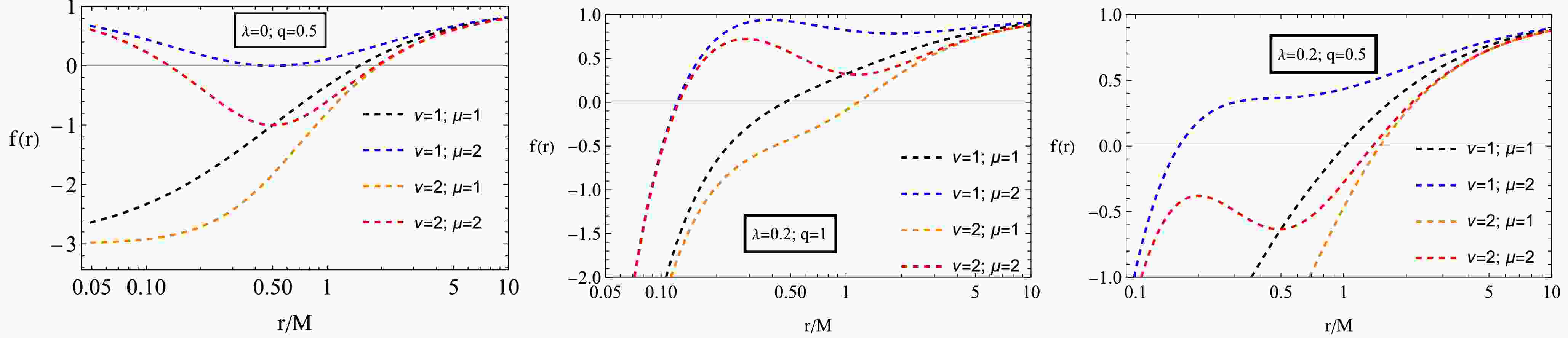
Figure 1 shows how the metric function $ f(r) $ around the black hole changes under different parameter influences. Increasing the NED parameters reduces spacetime curvature, making the black hole more stable. A higher charge strengthens the electromagnetic field, expanding the event horizon. PFDM causes the spacetime to extend and diminishes dynamic effects outside the black hole. These graphs highlight the interplay of these factors, providing insights into the structure of the spacetime surrounding the black hole.

Figure 1.  (color online) Radial dependence of the metric function $ f(r) $ for various values of q and λ and fixed values of μ and ν.

The given set of graphs in Fig. 2 represents the radius of the event horizon $ r_H $ versus different parameters (λ and q) for various combinations of the parameters ν and μ. The upper row shows $ r_H $ versus λ, and the bottom row shows $ r_H $ versus q. Each column corresponds to different values of ν and μ. The color panel on the right side of each graph shows the value of the third parameter, λ and q. The radius of the event horizon has a minimum value of a certain value of λ. The curves show all graphs. This minimum value varies according to the values of ν and μ. As the value increases, the initial value of the event horizon radius, $ r_H $, increases on the graphs. This shows that increasing ν causes the black hole to grow larger. An increase in the value of μ also increases the value of $ r_H $; however, this effect is weaker than the impact of ν. The U-shaped curves show the radius of the minimum event horizon as λ changes. This minimum value is reached at a certain value of λ, which varies for different parameters ν and μ. The graphs show that an increase in λ first decreases and then increases the radius of the event horizon. All graphs show that, with increasing q, the radius of the event horizon $ r_H $ generally decreases. This means that an increase in magnetic charge shrinks the radius of the black hole's event horizon.

Figure 2.  (color online) Event horizon radius for q and λ.

To explore the properties of spacetime, we may start by studying the scalar invariants of geometry around a compact gravitating object. Here, we analyze the Ricci scalar, square of the Ricci tensor, and Kretschmann scalar of the spacetime metric (1) given with the lapse function in Eq. (17).

The Ricci scalar, often known as the scalar curvature, is a fundamental measure of curvature in warped spacetime. The Ricci scalar measures the curvature of spacetime resulting from the presence of matter or energy, influenced by the intrinsic properties of the black hole and any external fields or modifications, such as PFDM and NED field parameters. The Ricci scalar also affects the orbits of particles in the accretion disk, such as the location of the ISCO, which sets the inner edge of the accretion disk and the orbital velocities, as well as the stability of particles in the disk. The emission properties of the accretion disk depend on the temperature and density profile of the disk, shaped by the spacetime curvature. In turn, changes in the Ricci scalar cause deviations in the temperature distribution, and thus, the emitted radiation will shift if the inner disk edge moves closer to or farther from the black hole. Observations of the accretion disk emissions can constrain the curvature properties and test deviations from standard GR, such as those introduced by PFDM and the NED field.

The Ricci scalar, the so-called scalar curvature, is one of the simplest curvature invariants of curved spacetime and is defined as $ R=g^{\mu\nu} R_{\mu\nu} $, where $ R_{\mu\nu} $is the Ricci tensor. The positive and negative values of the Ricci scalar correspond to the sunken and convex forms of the spacetime, respectively. After some simple mathematics, one may quickly get the following form of the Ricci scalar for the solution.

The square of the Ricci tensor provides a richer and more detailed measure of spacetime curvature than the Ricci scalar. It captures the interaction between matter-energy distributions and spacetime geometry, offering insights into high-energy astrophysical phenomena, gravitational wave dynamics, and cosmological structure formation. In addition, it is a crucial tool for testing and validating modified gravity theories. Consider the second scalar invariant, the so-called square of the Ricci tensor, responsible for the square of the energy-momentum tensor of a field in the spacetime of a black hole, and it is defined as $ {\cal R}=R_{\mu\nu}R^{\mu\nu}\equiv 1/(8\pi G)T_{\mu\nu}T^{\mu\nu} $ for the spacetime around black holes with the lapse functions given by Eq. (17). The square of the Ricci tensor takes the following form:

The Kretschmann scalar quantifies the total curvature of spacetime and highlights regions of strong-field effects. Near the black hole horizon, the behavior of $ {\cal K} $ provides insights into the impact of the PFDM and NED field parameters on tidal forces. At this point, we consider the Kretchmann scalar defined as $ {\cal K}=R_{\mu \nu \sigma \rho}R^{\mu \nu \sigma \rho} $. Usually, the square root of the Kretschmann scalar can be interpreted as an effective gravitational energy density $ \sqrt{{\cal K}} \sim \rho_M $. Therefore, one can easily calculate the Kretchmann scalar for the space-time metric in the form

Figure 3 shows how scalar invariants, such as the Ricci scalar, the squared Ricci tensor, and the Kretchman scalars, change with distance for various values of q. All invariants decrease rapidly with increasing r and approach the asymptotic value. An increase in the parameter ν causes a slight increase in the Ricci scalar invariant, an increase in the parameter μ causes a slight increase in the Ricci tensor invariant, and a decrease in the parameter μ causes a slight increase in the Kretchmann scalar invariant.

Figure 3.  (color online) Radial profiles of scalar invariants for varying values of q. Starting from the left in the top panel, the Ricci scalar, the square of the Ricci tensor, and the Kretchmann scalar, respectively.

Energy conditions are handy tools for discussing cosmological geometry and black hole spacetimes [99−101] in both GR [102] and modified gravity [103]. In the NED and PFDM models, it is essential to consider energy conditions to understand how gravity, electromagnetic fields, and DM behave. Energy conditions are fundamental constraints that ensure the physical consistency and stability of matter and energy in theoretical physics and cosmology.

These conditions impose restrictions on the stress-energy tensor, providing a framework to analyze gravitational phenomena without requiring detailed knowledge of the underlying matter dynamics. In the context of NED and PFDM, energy conditions are essential for understanding the interplay between gravity, electromagnetic fields, and DM [104].

The four primary energy conditions, WEC, NEC, DEC, and SEC, are particularly significant in studying spacetime properties. They ensure non-negative energy densities, causal energy flow, and physically realistic gravitational effects [105]. In addition, these conditions enable the derivation of significant results, such as singularity theorems, black hole topology theorems, and cosmic expansion constraints [106].

In NED, energy conditions regulate the behavior of nonlinear electromagnetic fields, preventing unphysical scenarios such as negative energy regions or superluminal propagation. In PFDM, they constrain the properties of DM, ensuring its compatibility with observational data and its role in shaping cosmic structures [104]. Together, these frameworks provide a robust foundation for exploring the intricate dynamics of spacetime and the evolution of the universe [107].

The standard energy conditions include NEC, WEC, SEC, and DEC, given as

Relevant quantities are deduced as

To examine the energy conditions of NED and PFDM in our case, we plot the unspecified quantities in Eq. (21) concerning the radial coordinate r in Fig. 4.

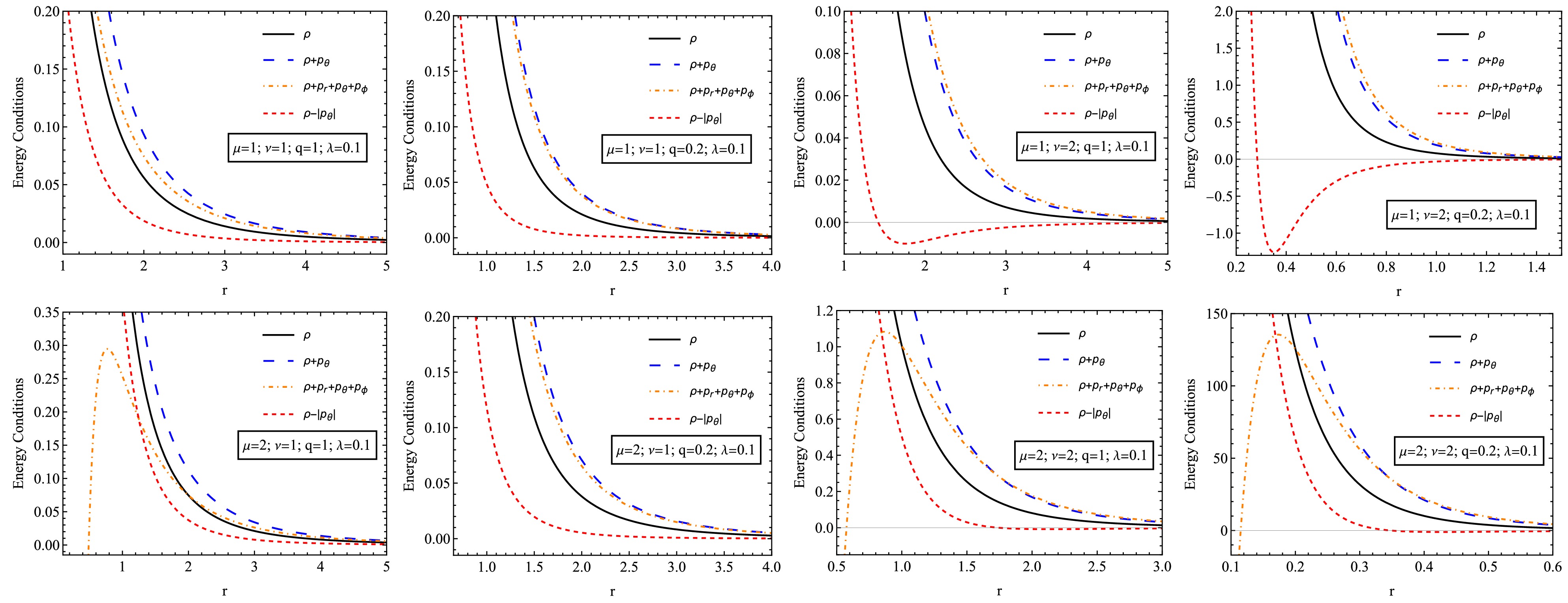
Figure 4.  (color online) Variation of ρ, $ \rho+p_\theta $, $ \rho+p_r+p_\theta+\rho_\phi $, and $ \rho-|p_\theta| $ versus r for NED and PFDM taking q = 1, q = 0.2, and λ = 0.1.

Figure 4 shows the different energy states and the dependence of the different energy states on r for different sets of parameters. The graphs depict the distribution of energy density and pressure under the influence of various parameters. As the radius increases, all energy conditions decrease while they attain higher values at smaller distances. An increase in charge reduces energy density, and in some cases, it may become negative, indicating a stronger spacetime curvature due to the electromagnetic field. PFDM expands spacetime and slows down energy distribution changes; however, some energy conditions may be violated at high values. The increase in NED parameters affects the internal structure of the black hole, stabilizing the energy density and pressure at larger distances. These results are crucial for understanding the distribution of matter, electromagnetic fields, and DM around the black hole, revealing the possible existence of exotic or unstable structures in certain cases.

Solving the equation $ f(r_h)=0 $, one can obtain the event horizon radius $ r_{h} $, with which the mass of the black hole can be expressed as

The Hawking temperature $ T_h $ is related to the surface gravity by

In Fig. 5, we plot the temperature of the black hole with the NED charge surrounded by PFDM. We can see that the black hole temperature increases and reaches a maximum before having a decreasing phase. Furthermore, this figure shows us that this maximum increases for higher values of the DM parameter λ. Note that the case "$ \lambda = 0 $" corresponds to the temperature of a black hole without DM. We write the first law of black hole thermodynamics from the black hole studied here and then find the entropy before computing the corrected entropy. The first law is expressed as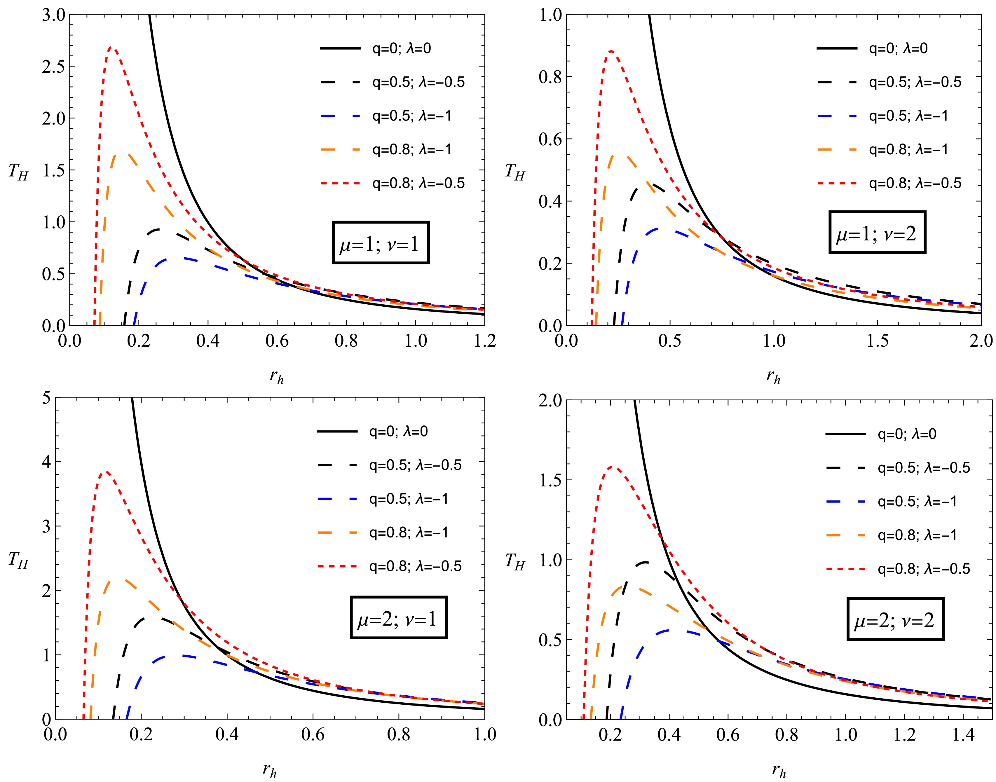

Figure 5.  (color online) Black hole temperature $ T_h $ as a function of the event horizon radius $ r_h $, showing the effects of the DM parameter λ and black hole charge q on thermal evolution.

where $ S_0 $ represents the entropy at the equilibrium without considering thermal fluctuation or the uncorrected entropy. Note that $ S_0 $, the magnetic charge q, and the DM parameter α form a complete set of extensible variables. $ T_h $ is the Hawking temperature at the horizon, $ \Phi_h $ is the potential, and $ \beta_h $ is the conjugating quantity of the DM parameter λ. Now, in the first expression of (25), we can find the formula of the uncorrected entropy $ S_0 $, given by

To compute this, we have to find $ \dfrac{\partial M}{\partial r_h} $ from Eq. (26). The obtained expression is as follows:

Introducing Eqs. (27) and (24) into Eq. (26), we get the black hole entropy at the equilibrium expressed as

Here, we can see that this result is the same as that obtained in the presence of quintessence DM found in Refs. [107, 108]. Consequently, we can say that PFDM does not affect the evolution of the entropy of a non-linear black hole.

Now, we compute the corrected entropy at the equilibrium S, for which the general formula is expressed as

Here, β is the corrected parameter with only two values. If $ \beta = 0 $, Eq. (29) describes the uncorrected entropy, and for $ \beta = 1/2 $, Eq. (29) represents the corrected entropy due to thermal fluctuation.

From the plots in Fig. 6, one can compare the corrected and equilibrium entropy for a given black hole. In the absence of the correction parameter β, the equilibrium entropy of the system is a linearly increasing function, as shown in the bottom. For the correction parameter $ \beta=1/2 $, the corrected entropy of the system always has a positive value, which is important for the system. The corrected entropy is a decreasing function below the critical horizon radius; however, above this point, it is always an increasing function. Therefore, for a larger black hole, the corrected entropy of the system is not significant as expected. However, for a smaller black hole system, the correction term significantly affects the entropy of the system owing to small thermal fluctuations.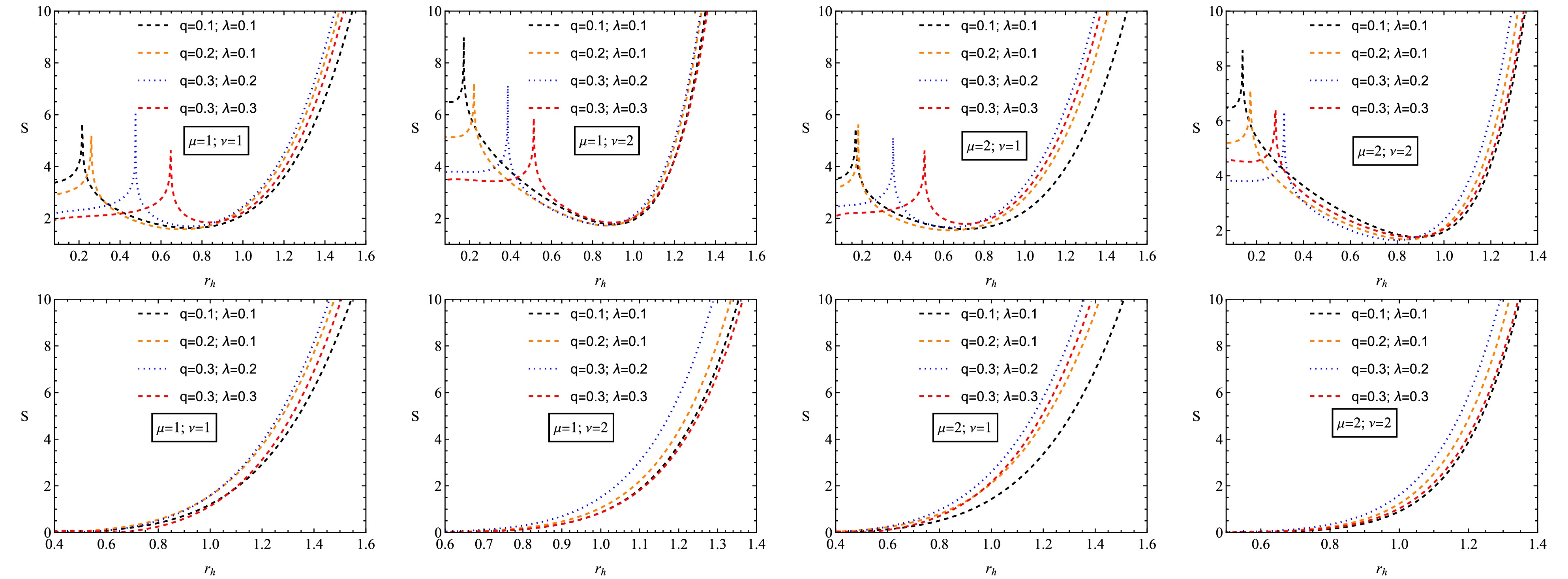

Figure 6.  (color online) Variation of entropy $ (S) $ with black hole horizon radius $ (r+) $ for different values of q and λ. Here, $ \beta = 0 $ (no correction) is the bottom panel, and $ \beta=1/2 $ (with correction) is the top panel.

The specific heat C at constant volume is given by

We need the relationship between the entropy S and the Hawking temperature $ T_h $, which involves the implicit dependence on $ r_h $.

We use

Then, we have

Finally, the specific heat is

After computing it, we get the following expression:

A black hole undergoes a second-order phase transition in phase transitions that lead the black hole to move from the stable phase $ (C > 0) $ to the unstable phase $ (C < 0) $.

Figure 7 presents the variation of the black hole heat capacity C as a function of the horizon radius, demonstrating the thermodynamic stability of the black hole solution under different values of the charge and the PFDM parameter. From the plots, one can observe the presence of discontinuities in the heat capacity, which indicate second-order phase transitions. These transitions separate different thermodynamic phases.

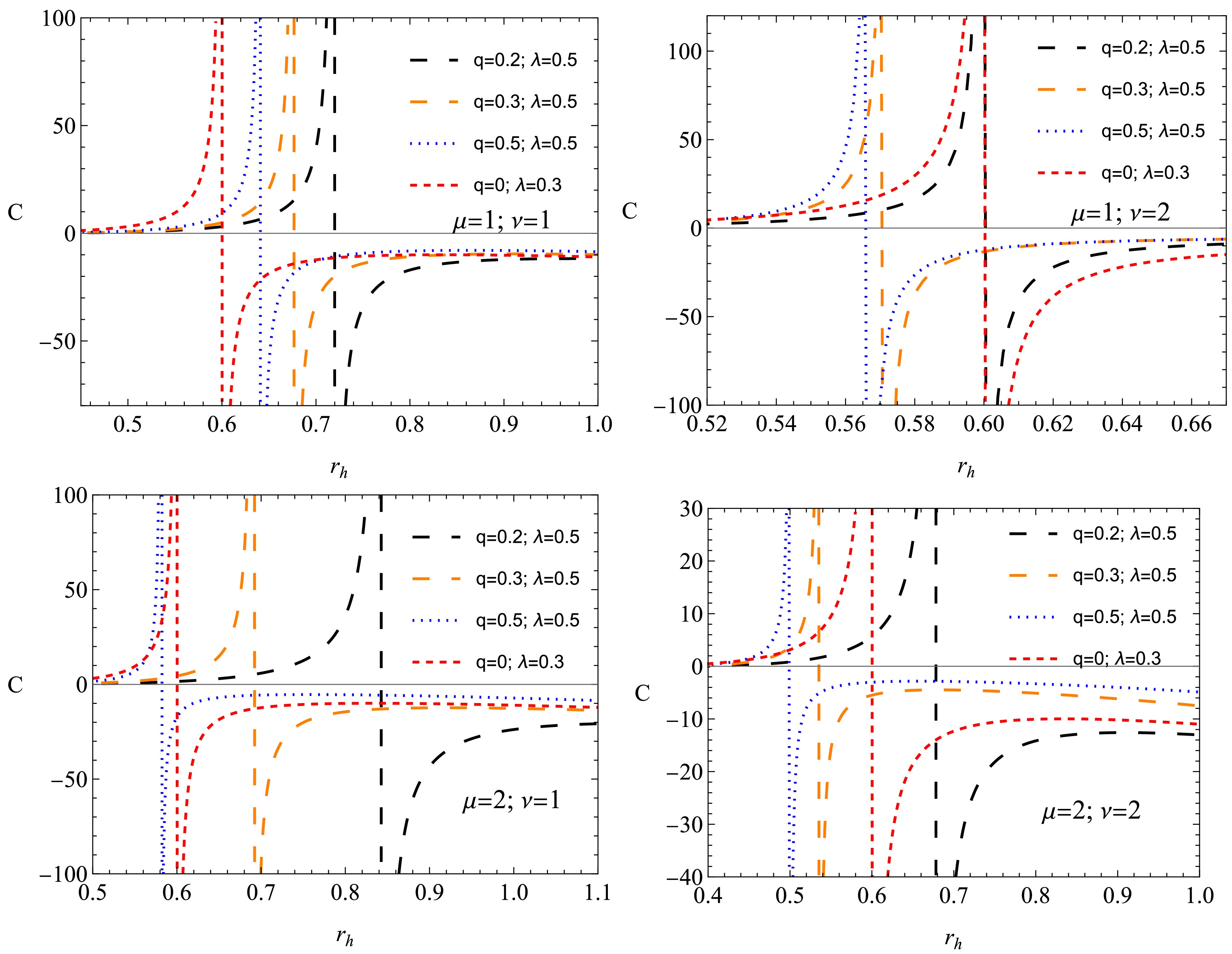
Figure 7.  (color online) Change in the heat capacity C of the non-linear black hole in the background of PFDM.

The heat capacity is negative for small black holes ($ r_h $ below the discontinuity point), implying that they are thermally unstable. This corresponds to an evaporating phase, in which the black hole loses mass via Hawking radiation. The heat capacity for large black holes ($ r_h $ above the transition point) becomes positive, signaling a stable equilibrium phase where the black hole can maintain thermal stability.

Increasing the black hole charge shifts the phase transition point, suggesting that stronger NED effects influence the thermodynamic structure of the black hole. The increase in charge leads to a more extended stable phase, reducing the likelihood of black hole evaporation. Increasing the PFDM parameter significantly alters the stability properties. A higher parameter value shifts the phase transition to a larger event horizon, implying that the presence of PFDM supports stability for larger black holes. This suggests that black holes embedded in PFDM environments are more resistant to evaporation than those in vacuum or standard DM models. From an astrophysical perspective, these findings suggest that black holes in environments with significant PFDM influence may have longer lifetimes, as the transition to a stable thermodynamic phase occurs at a larger horizon radius. Moreover, PFDM modifies the thermal response of the black hole, potentially affecting accretion disk dynamics, black hole mergers, and observational signatures related to thermal fluctuations.

A well-defined second-order phase transition strengthens the argument that such black holes exhibit non-trivial stability properties, distinguishing them from classical Schwarzschild or Reissner-Nordström black holes. Future observational tests, such as those involving black hole shadow measurements or X-ray spectra from accretion disks, could constrain the parameters q and λ based on their effects on stability and evaporation rates.

Neutral particle motion refers to the movement of particles that do not possess a net electric charge. Electric fields do not influence these particles because of their lack of charge. However, they may still be subject to other forces, such as gravitational, magnetic, or particle interactions. Examples of neutral particles include neutrons, neutrinos, and certain atoms or molecules with equal numbers of protons and electrons. Understanding the motion of neutral particles is crucial in various scientific fields, including nuclear physics, astrophysics, and materials science. Studying how neutral particles move and interact with their surroundings provides insight into the behavior of matter under different conditions and helps to understand fundamental processes in the universe.

The standard Lagrangian density for the neutral particle with rest mass m moving around a black hole can be written as

Owing to the existence of timelike and spacelike Killing vectors, one may introduce the conserved specific energy $ {\cal E} $ and specific angular momentum $ {\cal L} $ of the particle as follows:

The normalization condition governs the equations of motion for a test particle.

where $ \epsilon $ is $ 0 $ and $ -1 $ for massless and massive particles, respectively.

For neutral test particles, motion is governed by time-like geodesics of spacetime, and the motion equations can be found using Eq. (37). Considering Eq. (36), one may easily obtain the following equations of motion.

where K is the Carter constant associated with the total angular momentum.

Restricting the motion of the particle to the constant plane $\theta= \rm const$ and $ \dot{\theta}=0 $, the Carter constant takes the form $ K={\cal L}^2 $, and the equation of the radial motion can be expressed in the following standard form:

where the effective potential of the motion of neutral particles is defined as

Figure 8 shows the dependence of the effective potential on the radial distance under different values of black hole parameters. An increase in q and $\lambda $ is observed to lead to an increase in the potential. $\mu $ increases sharply as the parameter increases, indicating a stronger effect. As $\nu $ increases, the lines are slightly reduced; that is, the total value of the potential decreases.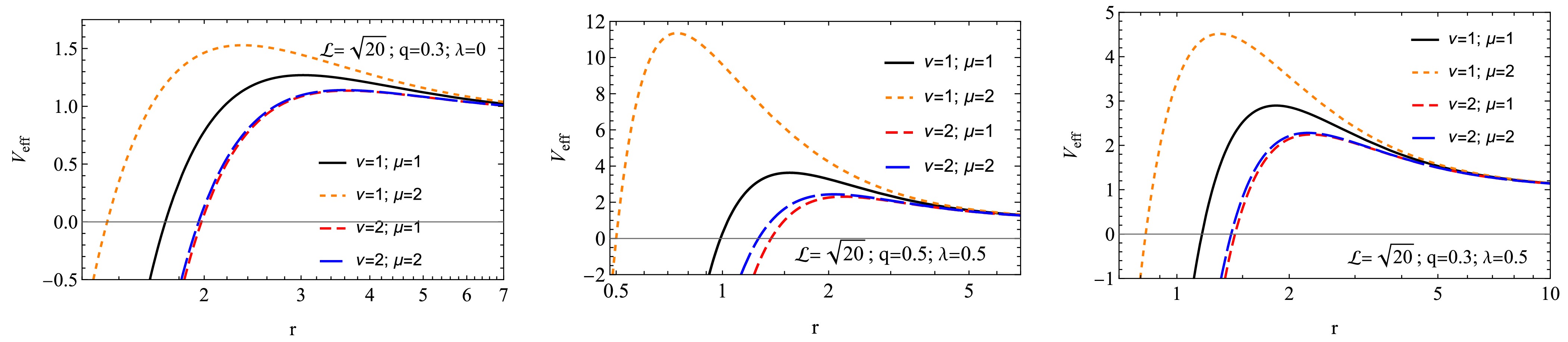

Figure 8.  (color online) Effective potential for radial motion of test particles with fixed specific axial angular momentum $ {\cal L}=\sqrt{20} M $ around a black hole.

To study the circular motion of the particles, we use the following conditions:

To find the values of angular momentum and energy of particles in circular orbits, we used the conditions given in Eq. (44) to obtain the following:

Figure 9 shows radial profiles of energy $ {\cal E} $ (top panel) and angular momentum $ {\cal L} $ (middle panel) corresponding to circular orbits. The bottom panel shows the dependence on energy and angular momentum. $ {\cal E} $ and $ {\cal L} $ decrease with increasing radial distance and then stabilize. A steady increase in energy is observed as the angular momentum increases. As the values of ν and μ increase, the energy $ {\cal E} $ and the angular momentum $ {\cal L} $ also increase.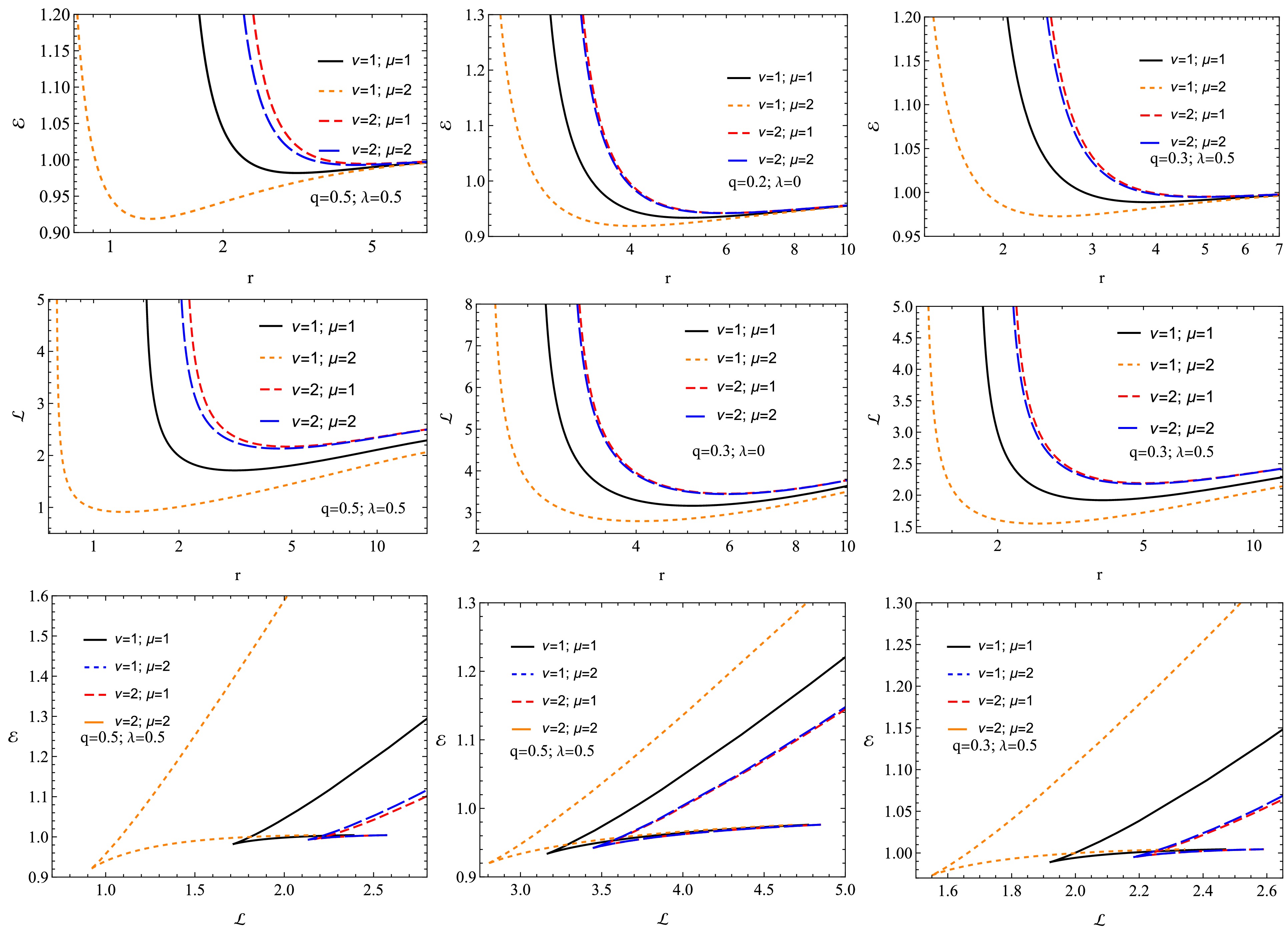

Figure 9.  (color online) Radial dependence of $ \cal L $ and $ \cal E $ varying with q for fixed λ (top panel). Plot of $ \cal L $ and $ \cal E $ for λ and q in the lower panel.

The stability condition of circular orbits of test particles around a central point of gravitating compact objects is described by the equation $ \partial_{rr}V_{\rm eff}\geq 0 $, while the ISCOs satisfy $ \partial_{rr}V_{\rm eff}= 0 $. This condition is often applied with the circularity condition in Eq. (44).

The condition $ \partial_{rr}V_{\rm eff}= 0 $ leads to the following equation, which is the solution with respect to the radial coordinate r that gives the ISCO radius.

The ISCO radius of the test particles can be calculated numerically by solving Eq. (46). The solution $r=r_{\rm ISCO}$ is shown in Fig. 10.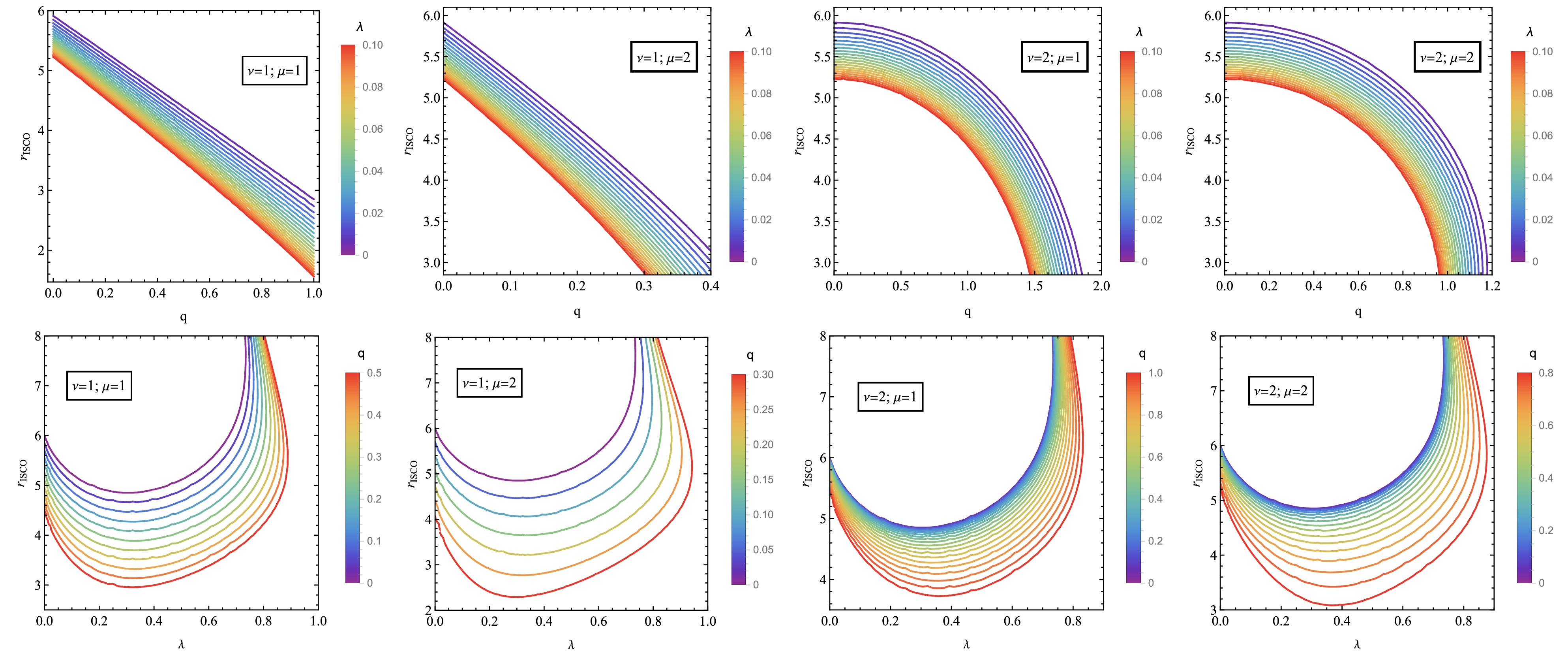

Figure 10.  (color online) Dependece of $r_{\rm ISCO}$ on λ for various values of q (left panel) and on q for varying values of λ (right panel).

The dependence of the ISCO radius on parameters q and λ is shown in Fig. 10. As μ and ν increase, the $r_{\rm ISCO}$ values become higher. As q increases, $r_{\rm ISCO}$ decreases, and as λ increases, $r_{\rm ISCO}$ first decreases and then increases.

The electrostatic fields and electromagnetic waves do not interact in linear electrodynamics. Conversely, in NED, a photon does not follow null geodesics; instead, it interacts with the field due to its nonlinearity. The "shifted-null" geodesics in the spacetime of the effective geometry for photons surrounding the black hole, governing the photon motion of black holes in spacetime obtained in GR coupled with NED are given as [50, 109−111]

in which

The corresponding photon eikonal equation in the effective geometry associated with a black hole may be stated as

In the above expression, $ k^\mu $ is the four-wave vector related to the photon four-momentum with the relation $ p^\mu=\hbar k^\mu $ (in Gaussian units, $ \hbar=1 $). In our previous studies [86, 112, 113], by graphical and numerical analyses, we demonstrated that the difference in shadow sizes, considering the interaction between the photon and the NED field, does not change significantly. The difference is smaller than the error in the data of EHT observations of Sgr A* ($ \sim 14 $%) and M87* (approximately 7.14%). Moreover, our primary focus in this study is probing the combined effects of spacetime parameters, the NED field charge, and the PFDM field on the black hole shadow shape and size.

Geodesic motion around a black hole is the most important aspect in forecasting the potential structure of a black hole shadow. Consider a test particle traveling around the black hole with a rest mass of $ m_0 $. Geodesics are easier to find if the constant of motion associated with the symmetry direction is determined. Let $ y^\sigma $ and $v^{\sigma}=\dfrac{{\rm d} x^{\sigma}}{{\rm d}\lambda}$ be the vectors along the symmetry direction and the tangent vector along the curve $ x^\sigma=x^\sigma(\tau) $, respectively, where τ is an affine parameter. If the trajectory $ x^\sigma $ is a geodesic [114], we may use the Killing vectors to get

The time-like Killing vector for a time-independent metric coefficient is provided by $ y^\sigma=(1,0,0,0) $, and the Killing vector for the ϕ direction may be expressed as $ y^{\sigma}=(0,0,0,1) $. By solving Eq. (51), we can establish the following relationship using the equation mentioned above as follows:

$ {\cal{E}} $ and $ {\cal{L}} $ indicate the relativistic energy and angular momentum per unit mass of a particle, respectively. The geodesic equations may now be determined using Eq. (52), as follows:

This becomes

The two remaining geodesic equations may be obtained using the Hamilton-Jacobi approach. Consequently, it may be inferred that

A proposed approach, such as the one mentioned in reference [115], would result in the following:

In Eq. (57), $ H_r $ and $ H_\theta $ represent the functions of r and θ, respectively. Introducing the Jacobi action (56) yields the Hamilton-Jacobi equation

in which

The geodesic equations of motion for a particle in the presence of a non-rotating black hole may be expressed using the relation $ H_{\theta}=\dfrac{\partial S}{\partial\theta}=\dfrac{\partial S_{\theta}}{\partial\theta} $ and $ H_{r}=\dfrac{\partial S}{\partial r}=\dfrac{\partial S_{r}}{\partial r} $.

Eq. (61) represents the geodesic equation along the θ direction, whereas Eq. (62) represents the geodesic equation along the r direction. Furthermore, the subsequent photon-traced geodesic equations are derived by assuming $ m_0^2=0 $ in the vicinity of the black hole [116].

Conversely, we may write Eq. (64) as

The symbol $ V_{\rm eff} $ represents the effective potential and is given by

Figure 11 plots the dependence of the various parameters that affect the radius of the black hole shadow. The shadows expand as q increases; that is, the radius of the shadows increases. This shows that the increase in the magnetic charge causes the photonsphere to expand. This increase is significant in each case; however, the sensitivity varies slightly depending on the values of $\mu $ and $\nu $. The shadows expand slightly as $\lambda $ increases; the effect of $\lambda $ is weaker than that of q but is still consistently noticeable. The shadow also expands as M increases; the larger the mass of the black hole, the larger its shadow. This indicates that the radius of the shadow directly depends on the mass.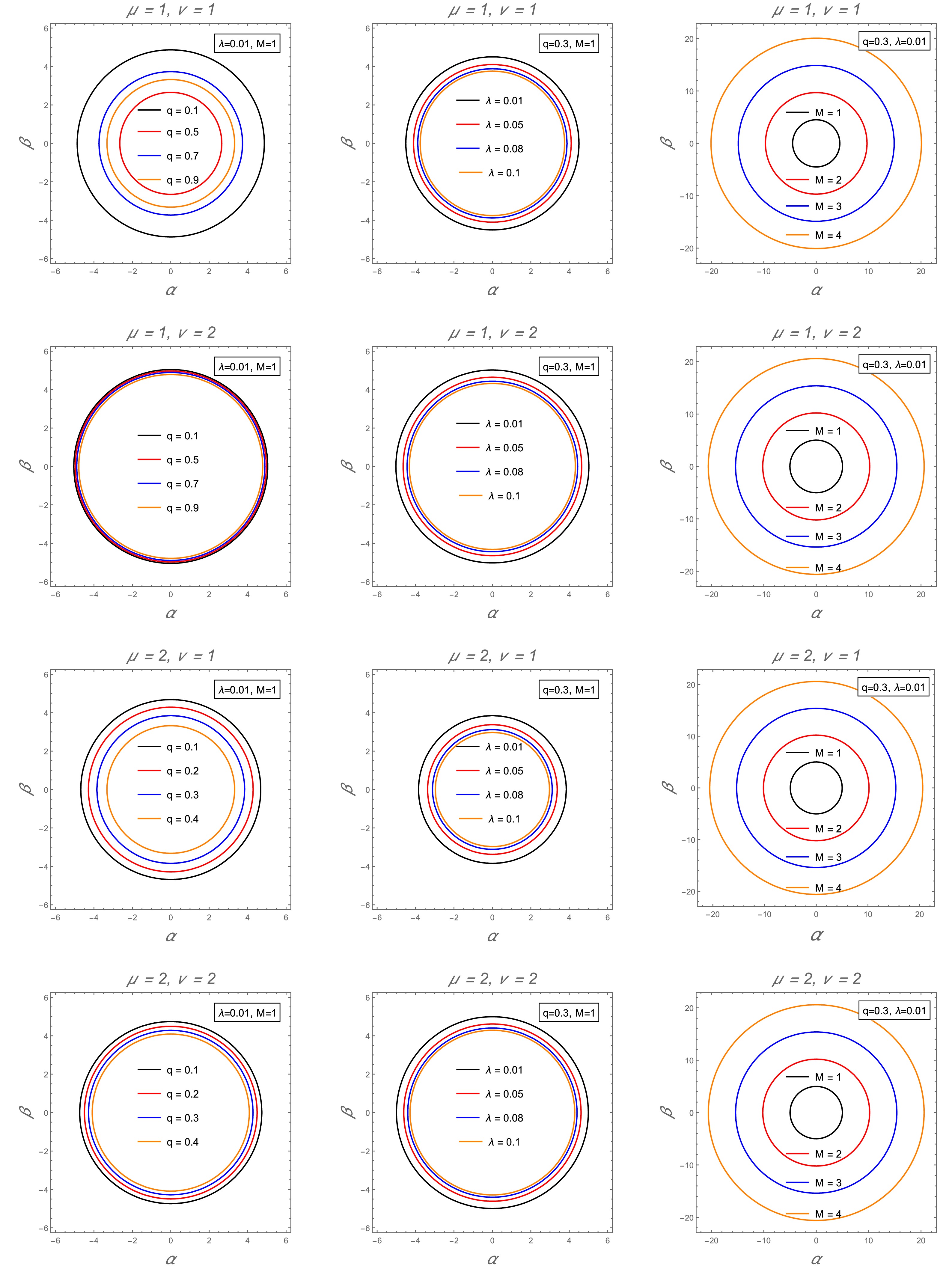

Figure 11.  (color online) Radial profile of the black hole shadow for parameters q (left panel), λ (middle panel), and M (right panel) at different combinations of parameters μ and $ \nu=1 $.

The following limitations aid us in identifying the unstable circular orbits:

In this context, $ r=r_p $ denotes the radius of a photon, and $ ' $ indicates the derivative concerning r. Hence, the equation $V_{\rm eff}(r_{p})=0$ indicates that

Equation (68) makes use of the Chandrasekhar constant definition [115], which is $ \xi={K}/{{\cal{E}}^{2}} $ and $ \eta={\cal{L}}/{\cal{E}} $. Similarly, $ V'_{\rm eff}(r_p)=0 $, resulting in

Figure 12 shows how the photonsphere radius rph varies for various combinations of the parameters λ and q as well as ν and μ. The top row shows the relationship between rph and λ, and the bottom row shows the relationship between rph and q. Each column corresponds to a specific set of ν and μ values. The color bar to the right of each plot shows the third variable parameter λ or q. The graphs reveal the minimum value of λ for the event horizon radius, which depends on the values of ν and μ. As ν increases, the initial value of rph also increases, indicating that a larger ν leads to a larger black hole. Although increasing μ also increases rph, its effect is weaker than that of ν. The U-shaped curves emphasize that rph reaches a minimum at a certain λ that shifts with different values of ν and μ. In general, rph first decreases and then increases with increasing λ. By contrast, all plots consistently show that increasing q leads to a decrease in rph, indicating that the high magnetic charge squeezes the event horizon.

Figure 12.  (color online) Dependece of $ r_{ph} $ on λ for various values of q (top panel) and on q for varying values of λ (bottom panel).

Imagine a massless particle, such as a photon, released by an object traveling toward the black hole between an observer and a brilliant object. Photon paths may result in (a) scattering away from the black hole, (b) falling into the black hole, or (c) a critical geodesic dividing (a) and (b). The scattering of a photon from the black hole is visible to the viewer during this entire process. However, a dark zone will develop when a photon enters the black hole. We call this dark zone the shadow of the black hole. Our primary objective in this part is to investigate the shadow emitted in PFDM spacetime by the black hole. First, we must specify the celestial coordinates [81, 112, 117] for this purpose as

In this context, α represents the apparent perpendicular distance of the shadow from the axis of symmetry, whereas β represents its projection on the equatorial plane. The variable θ denotes the inclination angle between the axis of symmetry and the observer's line of sight, while $ r_0 $ indicates the distance between the black hole and the observer. The values of the derivatives $ {\rm d}\phi/{\rm d}r $ and $ {\rm d}\theta/{\rm d}r $ may be determined by using the geodesic equations in the following manner:

When Eqs. (72) and (73) are solved for $ r\rightarrow \infty $, the expression for the celestial coordinates (70) assumes the following form [118, 119]:

The preceding equations are further simplified when $ \theta=\pi/2 $ is substituted in

Consequently, the expression of the shadow radius in the celestial plane ($ \alpha, \beta $) may be computed as follows:

In Eq. (76), $ R_s $ stands for the radius of the black hole shadow while it is not revolving.

In this section, we examine the dependence of the PFDM parameter λ and q on the shadow images of the black holes M87* and Sagittarius A* (Sgr. A*) using Event Horizon Telescope (EHT) observations. Our analysis is limited to the non-rotating case, since the rotation parameter a of Sgr. A* is sufficiently small to have a negligible effect on the shadow radius [120]. Furthermore, distinguishing between a Kerr black hole ($ a = 0.60\;\rm M $) and a non-rotating extended black hole for M87* using shadow images alone is shown to be challenging. This conclusion is supported by general-relativistic magnetohydrodynamic simulations and radiative transfer calculations that generate synthetic shadow images for direct comparison with EHT observations [121].

Furthermore, as noted in Ref. [122], the shadow size of M87* is observed to lie in the range of $3\sqrt{3}(1 \pm 0.17)\;\rm M$.

Regardless of whether the underlying model assumes spherical symmetry or axisymmetry. This observation provides a strong basis for constraining theoretical models of black holes in alternative theories of GR and gravity. By comparing theoretical predictions of the shadow radius from our model with EHT observational data, we attempt to determine the allowable ranges for the parameter q and other relevant physical parameters. This approach allows us to probe the interplay between NED, DM, and gravitational effects around black holes in the strong field regime.

The EHT collaboration reported the following data for M87*: the angular diameter of the shadow is $ \theta_\text{M87*} = 42 \pm 3 \:\mu $as, the distance to M87* is $ D = 16.8 $ Mpc, and the mass of M87* is $M_\text{M87*} = 6.5 \pm 0.90 \times 10^9 \: \rm M_\odot$ [123]. For Sgr. A*, recent EHT results provide the angular diameter of the shadow as $ \theta_\text{Sgr.A*} = 48.7 \pm 7 \:\mu $, the distance to Sgr. A* as $ D = 8277 \pm 33 $ pc, and the black hole mass as $M_\text{Sgr. A*} = 4.3 \pm 0.013 \times 10^6 \:\rm M_\odot$ (VLTI) [124, 125].

Using the provided data, the shadow diameter in units of mass can be calculated using the formula [126]

The theoretical shadow diameter is given by $ d_\text{sh} = 2R_\text{sh} $. Applying the above expression, we find the shadow diameter for M87* to be $d^\text{M87*}_\text{sh} = (11 \pm 1.5)\;\rm M$ and that for Sgr. A* to be $d^\text{Sgr.A*}_\text{sh} = (9.5 \pm 1.4)\;\rm M$.

The relationship between q and λ affecting the black hole shadow size is shown in Fig. 13. The graphs are drawn based on EHT observational data for M87* and Sgr A*, with the $ q/M $ axis representing the charge-to-mass ratio and the $ d_{\text{sh}}/M $ axis representing the shadow diameter-to-mass ratio. The black lines correspond to $ \lambda = 0 $, representing the scenario where the effect of DM is not considered. The red dashed lines show the variation in shadow size when $ \lambda = 0.03 $, illustrating how the presence of DM influences the shadow. Evidently, as $ q/M $ increases, the shadow diameter decreases and this reduction occurs more rapidly when λ is present. The confidence intervals $ 1\sigma $ and $ 2\sigma $ represent the observational data provided by the EHT. When λ is absent, the black lines mostly fall within the $ 1\sigma $ confidence interval, indicating that the model without the influence of DM aligns well with the EHT observations. By contrast, the red dashed lines representing the case where λ is present mostly fall within the $ 2\sigma $ interval, suggesting the possible influence of DM. However, this influence is not as strong within the $ 1\sigma $ range. Thus, the graphs clearly show how the parameters q and λ affect the black hole shadow size. An increase in charge and the DM parameter reduces the shadow size. Based on EHT observations, the absence of λ corresponds more closely to the $ 1\sigma $ interval, indicating a minimal influence of DM. However, the presence of λ aligns with the $ 2\sigma $ interval, suggesting the possible existence of DM.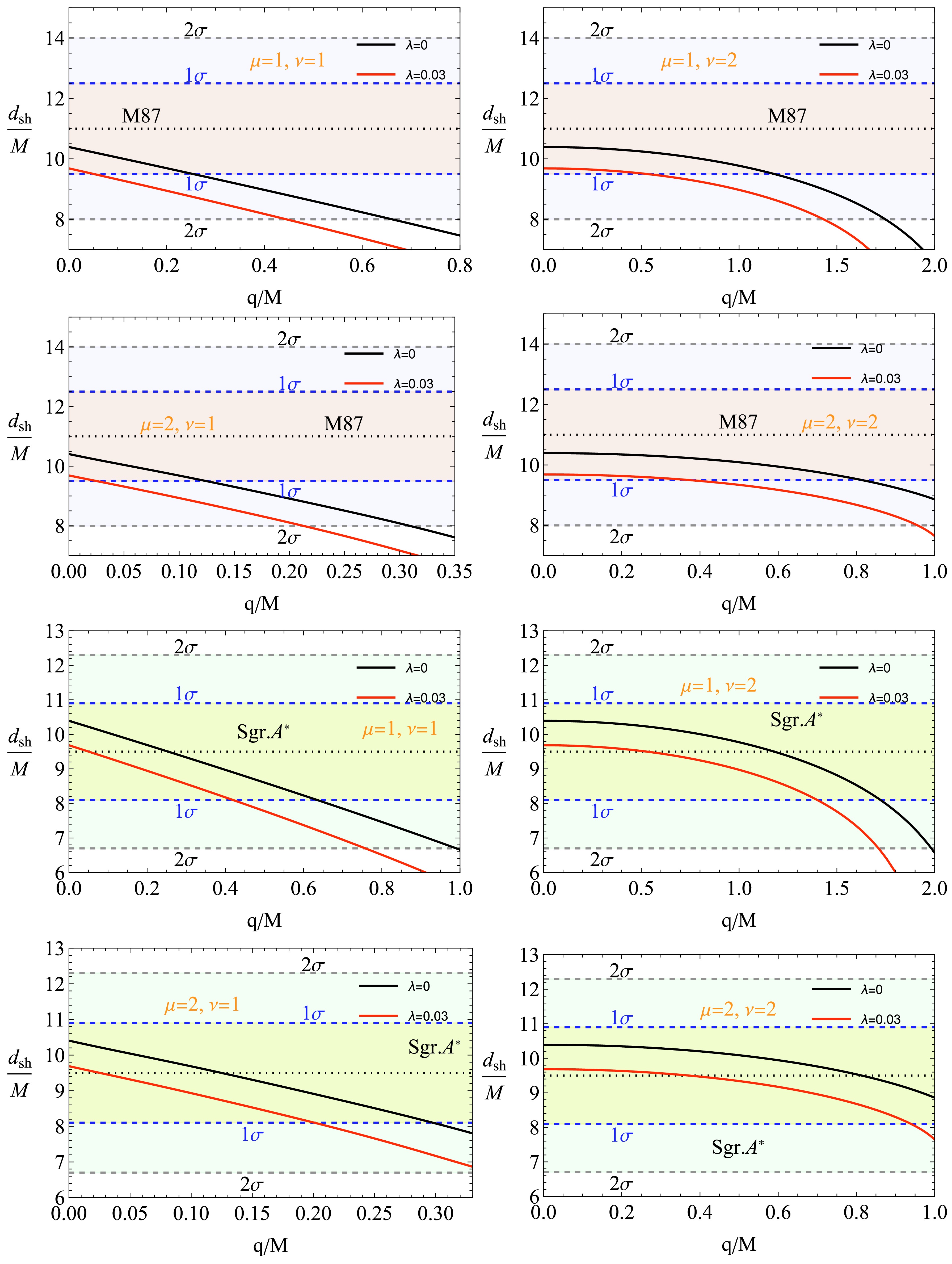

Figure 13.  (color online) The plot shows the constraints for q. The corresponding values of q at the mean, $ 1\sigma $, and $ 2\sigma $ confidence levels are shown.

This study investigated the properties of black holes in GR coupled to NED in the presence of PFDM. The main results obtained across different sections are summarized below. A singular black hole solution was derived, incorporating the effects of NED and PFDM. The energy conditions, including the WEC, NEC, SEC, and DEC, were examined. All energy conditions were observed to decrease as the radius increased. Higher charge values reduced the energy density and sometimes led to negative energy densities, indicating the influence of strong spacetime curvature. The PFDM parameter increase slowed energy distribution changes, whereas NED parameters stabilized the energy density at more considerable distances.

The thermodynamic properties, including temperature, entropy, and specific heat, were analyzed. The specific heat capacity transitioned from positive to negative values, suggesting stability and phase transition behavior in particular parameter ranges. PFDM and NED modified the black hole’s Hawking temperature, indicating changes in its thermodynamic equilibrium.

The geodesic motion of neutral particles was studied, focusing on circular orbits. ISCO was derived from the black hole parameters. Increasing PFDM parameters was observed to shift the ISCO radius, while higher charge values reduced it.

The black hole shadow was computed under different parameter values, revealing how PFDM and NED influence its size and shape. The radius of the shadow increased with higher values of PFDM parameters but decreased with increasing charge. The computed results provide insights into how black hole imaging techniques can place future observational constraints on these parameters.

The results demonstrated that the influence of NED and PFDM on black hole properties shows the dependence of energy conditions on charge and PFDM parameters. Notable deviations from standard GR expectations were identified. In addition, the results indicate the variations in temperature, entropy, and specific heat, highlighting regions of stability and instability. Finally, they present the shifts in circular orbits and ISCO under different parameter values, showing a direct influence of PFDM and NED. We have also demonstrated how to modify observational characteristics such as the shadow radius, which is crucial for astrophysical applications.

The study provides a new framework for understanding black holes in alternative gravity models with DM interactions. The findings suggest that black holes in PFDM environments exhibit modified thermodynamic and observational properties. Future black hole imaging and gravitational wave observations can test these properties. Further research is needed to explore the role of rotation and higher-order corrections in these models. The results can be extended to analyze accretion disk properties and their implications for high-energy astrophysics. In conclusion, this study contributes to understanding black holes in modified gravity scenarios and offers potential pathways for observational tests using astrophysical and cosmological data.

Our analysis of the black hole shadow in the presence of NED and PFDM has provided key insights into how these parameters affect the observable shadow radius. Comparing our results with the EHT measurements of M87* and Sgr A*, we find that PFDM contributes to an increase in the shadow size. Concurrently, NED effects introduce modifications that can reduce it. The interplay of these effects allows us to place constraints on the model parameters, ensuring that deviations from GR remain within observational limits. Precisely, we determine that the values of the NED charge parameter q and PFDM density parameter λ must be finely tuned to reproduce the observed shadow sizes within the 7.14% (M87) and 14% (Sgr A) uncertainty ranges reported by EHT. These constraints provide a novel way to test alternative gravity models and highlight the potential detectability of PFDM signatures in future high-precision black hole imaging experiments.