


 Abstract
 HTML
HTML Reference
 Related
 PDF
PDF


-
Pairing correlations are of special importance in nuclear structure theory. They influence many nuclear properties such as deformation and moments of inertia. The pairing between like-particles (i.e., protons or neutrons) has been widely studied since the end of the 1950s when the Bardeen, Cooper, and Schrieffer (BCS) theory of superconductivity [1] was adapted to nuclear physics [2].
In
$ N\simeq Z $ nuclei, a large overlap exists between neutron and proton wave functions. Thus, in addition to the pairing between like-particles, a neutron-proton (np) pairing exists. It may be of two different types, namely, isovector pairing (T=1) and isoscalar pairing (T=0). The first theoretical studies on np pairing by Goswami et al. [3−6] date to the 1960s. However, they were somewhat abandoned for many years because the nuclei in which this type of pairing exists could not be observed experimentally. When the experimental study of these nuclei was made possible with the advent of radioactive ion beams, np pairing was the subject of a marked revival of interest over the last 25 years in both theoretical and experimental studies [7]. Many methods have been developed to describe both types of np pairing. A generalized BCS approach is often used (see e.g., [8−14]; for a review, see Refs. [15−16]), because of its ease of use. It was applied to study various nuclear quantities such as the moment of inertia [17] and one-proton and two-proton separation energies [18].As the BCS method breaks the particle-number conservation symmetry, several studies have been devoted to the particle-number fluctuations in np pairing, such as the Lipkin-Nogami method [19−23], which conserves approximately the particle number. The restoration of the broken symmetry may also be performed using various approaches as particle-number projection methods either before (see e.g., [24−26]) or after the variation (see e.g., [27−31]). These methods have been applied to study various nuclear observables such as electric quadrupole moments [32], beta transition probabilities [33, 34], charge, proton, and neutron systems and matter radii [35], moments of inertia [36], and spectroscopic factors of various reactions [37−38].
Recently, a model based on the generator coordinate method has been developed to include np pairing correlations. It was applied to the magnetic properties of
$ N=Z $ odd-odd nuclei [39].Another possible approach consists of describing
$ N=Z $ systems with np pairing using α-like quartets (see Ref. [40] and references therein).Moreover, the np pairing effect may be analyzed using a shell model mean-field in which the isovector pairing Hamiltonian can be built using generators of the quasispin O(5) group [41, 42]. A shell-model-like approach based on the relativistic density functional theory may also be used [43].
A completely different study method consists of describing the np pairing correlations on quantum computers using a variational quantum eigensolver approach [44].
Nevertheless, all the cited methods describe systems at zero temperature. The oldest method for considering the pairing correlations in heated nuclei is the finite temperature BCS (FTBCS) approach, which is also among the most used [45−49]. Some methods based on this approach are the BCS-average [50−52] and particle-number projection methods, either of PBCS or FBCS types [53−57]. Another approach is the Hartree-Fock-Bogoliubov (HFB) method [58−65], which may be also in its relativistic form [66]. In addition to the aforementioned models, others exist, such as random-phase-approximation [67−71], the covariant density functional theory [72−76], Matsubara formalism [77], the self-consistent Green's function approach [78], and the generalized Lipkin-Nogami model [79]. For a review, see Ref. [80].
Another method to study the thermal pairing effect is the path integral technique in the framework of the shell-model Monte-Carlo method (SMMC) [81−83] or in a more convenient form in the static-path approximation [84−90]. Let us also cite the work of Fletcher [91], who has shown that the path integral formalism enables the retrieval of FTBCS results using some approximations.
However, all these studies involve pairing between like-particles. Only few studies were devoted to np pairing correlations at finite temperature. The most used methods are the shell model [92−95] and SMMC [96−97]. More recently, the finite temperature np quasiparticle-random-phase-approximation was used to study Gamow-Teller excitations [98]. In Ref. [99], the phase diagrams for np superfluidity was investigated in asymmetric nuclear matter with the inclusion of the angular dependence of the pairing gap.
In Refs. [100−102], the np temperature dependent isovector pairing correlations were studied in the framework of the path integral technique using a generalization of the Fletcher method, whereas the isovector plus isoscalar correlations were studied in Ref. [103].
Recently, we proposed a method for the treatment of pairing correlations between like-particles at finite temperature within the path integral formalism based on the square-root extraction of the pairing term in the Hamiltonian of the system [104]. The aim of the present work is to generalize this method to np pairing. For simplicity, we consider only isovector pairing correlations.
The remainder of the paper is organized as follows: Secs. II and III present the Hamiltonian of the system and the derivation of the partition function, respectively. The gap equations and expressions for the statistical quantities are established in Sec. IV. Numerical results are presented and discussed in Sec. V. The main conclusions are given in the final section.
-
Let us consider a system of N neutrons and Z protons. For isovector pairing, it can be described in the second quantization and isospin formalism using the total Hamiltonian [3, 11, 15, 16]
$ \begin{aligned}[b] \mathcal{H} =\;&\sum_{\nu>0,t}\varepsilon_{\nu t}\left( a_{\nu t}^+a_{\nu t}+a_{\tilde{\nu}t}^+a_{\tilde{\nu}t}\right) \\ & -\sum_{t}G_{tt}P_{t}^+P_{t}-G_{np}P_{np}^+P_{np}. \end{aligned} $

(1) In this expression,
$ \varepsilon_{\nu t} $ represents the single-particle energies, and$ t=n,p $ is the isospin component.$ a_{\nu t}^{+} $ $ \left( a_{\nu t}\right) $ is the creation (annihilation) operator of a nucleon in the$ \vert \nu t\rangle $ state. The state$ \vert \tilde{\nu}t\rangle $ is the time-reversed state of$ \vert \nu t\rangle $ .$ G_{tt^{\prime}} $ ($ t,t^{\prime}=n,p $ ) denotes the pairing-strength that are assumed to be constant. We also assume that$ G_{np}=G_{pn} $ .The operators
$ P_{t}^{+} $ and$ P_{np}^{+} $ are defined by$ \begin{align} P_{t}^+ & =\sum_{\nu>0}a_{\nu t}^+a_{\tilde{\nu}t}^+\text{ } \end{align} $

(2) $ \begin{align} P_{np}^+ & =\sum_{\nu>0}\left( a_{\nu p}^+a_{\tilde{\nu}n} ^++a_{\nu n}^+a_{\tilde{\nu}p}^+\right) . \end{align} $

(3) Indeed, given the presence of the isospin quantum number t in the expression of
$ \mathcal{H} $ , nucleons can interact with each other and create proton-proton, neutron-neutron, and neutron-proton pairs while respecting the Pauli principle.To conserve, on average, the particle numbers, we define the auxiliary Hamiltonian as
$ H=\mathcal{H}-\sum\limits_{t}\lambda_{t}N_{t} $

(4) where
$ \lambda_{t} $ is the Fermi level, and$ N_{t} $ is the particle-number operator of a like-particles system (neutron or proton) defined by$ N_{t}=\sum\limits_{\nu>0}\left( a_{\nu t}^+a_{\nu t}+a_{\tilde{\nu}t} ^+a_{\tilde{\nu}t}\right) $

(5) H may then be expressed as
$ H=H_{0}+H_{1} $

(6) where we use the notations
$ H_{0}=\sum\limits_{\nu>0,t}\tilde{\varepsilon}_{\nu t}\left( \eta_{\nu t} +\eta_{\tilde{\nu}t}\right) $

(7) $ H_{1}=\sum\limits_{t}H_{tt}+H_{np} $

(8) $ H_{tt}=-G_{tt}P_{t}^+P_{t}\text{ , }H_{np}=-G_{np}P_{np}^+P_{np} $

(9) $ \tilde{\varepsilon}_{\nu t}=\varepsilon_{\nu t}-\lambda_{t}\text{ , } $

(10) $ \eta_{\nu t}=a_{\nu t}^+a_{\nu t}\text{ }. $

(11) Ref. [104] showed that
$ H_{tt} $ may take the form$ H_{tt}=-G_{tt}R_{tt}^{2} $

(12) with
$ R_{tt}=\sum\limits_{\nu>0}\eta_{\nu t}\eta_{\tilde{\nu}t}B_{\nu t}, $

(13) where
$ B_{\nu t}=\prod\limits_{\substack{j>0\\j\neq\nu}}\mathcal{S}_{jt}\text{ , }\mathcal{S}_{jt}={\rm i}\left( a_{jt}+a_{jt}^+\right) \left( a_{\tilde{j}t}+a_{\tilde{j}t}^+\right) . $

(14) The operator
$ H_{np} $ may be expressed as$ H_{np}=-G_{np}R_{np}^{2} $

(15) where
$ R_{np}=\sum\limits_{\nu>0}\left[ \eta_{\nu n}\eta_{\tilde{\nu}p}B_{\nu n\tilde{p}}+\eta_{\nu p}\eta_{\tilde{\nu}n}B_{\nu p\tilde{n} }\right] $

(16) with
$ \begin{align} B_{\nu n\tilde{p}} & =\left( a_{\tilde{\nu}n}+a_{\tilde{\nu} n}^+\right) \left( a_{\nu p}+a_{\nu p}^+\right) \prod \limits_{\substack{j>0\\j\neq\nu}}\mathcal{S}_{jn}\text{ }\mathcal{S}_{jp} \end{align} $

(17) $ \begin{align} B_{\nu p\tilde{n}} & =\left( a_{\tilde{\nu}p}+a_{\tilde{\nu} p}^+\right) \left( a_{\nu n}+a_{\nu n}^+\right) \prod \limits_{\substack{j>0\\j\neq\nu}}\mathcal{S}_{jn}\text{ }\mathcal{S}_{jp}. \end{align} $

(18) The calculation details are given in Appendix A.
-
The grand partition function is given by
$ Z=\text{Tr}{\rm e}^{-\beta H}, $

(19) where β is the inverse of the temperature T of the system, and Tr is the trace over all the states of the system. Z is also given by
$ Z=\text{Tr}{\rm e}^{-\beta H_{0}}\mathsf{S}\left( \beta\right) $

(20) where the operator
$ \mathsf{S}\left( \beta\right) $ is defined by$ \mathsf{S}\left( \beta\right) ={\rm e}^{\beta H_{0}}{\rm e}^{-\beta H}. $

(21) It may be expressed formally as [104]
$ \mathsf{S}\left( \beta\right) =T_{\tau}\exp\left( \int_{0}^{\beta} H_{1}\left( \tau\right) {\rm d}\tau\right) $

(22) $ T_{\tau} $ is the chronological operator.Using the definition (8) of
$ H_{1} $ ,$ \mathsf{S}\left( \beta\right) $ becomes$ \begin{aligned}[b] \mathsf{S}\left( \beta\right) =\;&T_{\tau}\text{ }\exp\left( \int _{0}^{\beta}H_{nn}\left( \tau\right) {\rm d}\tau\right) \\ & \times\exp\left( \int_{0}^{\beta}H_{pp}\left( \tau\right) {\rm d}\tau\right) \exp\left( \int_{0}^{\beta}H_{np}\left( \tau\right) {\rm d}\tau\right) \end{aligned} $

(23) where we have assumed that
$ H_{nn} $ and$ H_{pp} $ commute with$ H_{np}. $ Indeed, the commutators$ \left[ H_{tt},H_{np}\right] , $ are proportional to the products$ G_{tt}G_{np} $ , which are small compared with the single-particle energies.Appendix B shows that Z takes the form
$ \begin{aligned}[b] Z =\;&\frac{1}{\pi^{3/2}\sqrt{G_{nn}G_{pp}G_{np}}}\int {\rm d}\Delta_{nn} {\rm d}\Delta_{pp}{\rm d}\Delta_{np}\exp\\&\times\left\{ -\beta\left[ \frac{\left\vert \Delta_{nn}\right\vert ^{2}}{G_{nn}}+\frac{\left\vert \Delta_{pp}\right\vert ^{2} }{G_{pp}}+\frac{\left\vert \Delta_{np}\right\vert ^{2}}{G_{np}}\right] \right\} Tr\exp\\&\times\left( -\beta\sum\limits_{\nu}h_{\nu np}\right) \end{aligned} $

(24) with
$ \begin{aligned}[b] h_{\nu np} =\;&\tilde{\varepsilon}_{\nu n}\left( \eta_{\nu n} +\eta_{\tilde{\nu}n}\right) +\tilde{\varepsilon}_{\nu p}\left( \eta_{\nu p}+\eta_{\tilde{\nu}p}\right) +2\Delta_{nn}\eta_{\nu n} \eta_{\tilde{\nu}n}B_{\nu n}\\&+2\Delta_{pp}\eta_{\nu p}\eta_{\tilde{\nu }p}B_{\nu p} +2\Delta_{np}\left( \eta_{\nu n}\eta_{\tilde{\nu}p}B_{\nu n\tilde{p}}+\eta_{\tilde{\nu}n}\eta_{\nu p}B_{\nu p\tilde{n} }\right) \end{aligned} $

(25) In the following, we will admit that the
$ h_{\nu np} $ and$ h_{\mu np} $ operators commute when$ \nu\neq\mu. $ (see Appendix C for the justification.)We then have
$ \text{Tr}\exp\left( -\beta\sum\limits_{\nu}h_{\nu np}\right) =\prod\limits_{\nu }\text{Tr}\exp\left( -\beta h_{\nu np}\right) . $

(26) All the operators in the expression for
$ h_{\nu np} $ commute with each other and act on different spaces. The eigenvalues of operators$ \eta_{\nu t} $ are$ 0 $ and$ 1 $ , and those of$ \eta_{\tilde{\nu}t} $ are the same. The operators$ B_{\nu t} $ ,$ B_{\nu n\tilde{p}} $ , and$ B_{\nu\tilde{n}p} $ each have the eigenvalues$ -1 $ and$ 1 $ . Subsequently, after some algebra, the partition function takes the form$\begin{aligned}[b] Z=\;&\frac{1}{\pi^{3/2}\sqrt{G_{nn}G_{pp}G_{np}}}\int {\rm d}\Delta_{nn}{\rm d}\Delta _{pp}{\rm d}\Delta_{np}\exp\\&\times\left\{ -\beta\left[ \frac{\left\vert \Delta _{nn}\right\vert ^{2}}{G_{nn}}+\frac{\left\vert \Delta_{pp}\right\vert ^{2} }{G_{pp}}+\frac{\left\vert \Delta_{np}\right\vert ^{2}}{G_{np}}\right] \right\}\\&\times \prod\limits_{\nu}\left( 8A_{\nu}\right) \end{aligned}$

(27) where
$ A_{\nu} $ is defined by$ \begin{aligned}[b] A_{\nu} =\;&2\left( 1+2{\rm e}^{-\beta\tilde{\varepsilon}_{\nu n}} +{\rm e}^{-2\beta\tilde{\varepsilon}_{\nu n}}\cosh2\beta\Delta_{nn}\text{ }\right)\\&\times \left( 1+2{\rm e}^{-\beta\tilde{\varepsilon}_{\nu p}}+{\rm e}^{-2\beta \tilde{\varepsilon}_{\nu p}}\cosh2\beta\Delta_{pp}\text{ }\right) \\ & +4\left( \cosh2\beta\Delta_{np}-1\right) \Big[ {\rm e}^{-\beta\left( \tilde{\varepsilon}_{\nu n}+\tilde{\varepsilon}_{\nu p}\right) }+{\rm e}^{-\beta\left( 2\tilde{\varepsilon}_{\nu n}+\tilde{\varepsilon }_{\nu p}\right) }\\&\times\cosh2\beta\Delta_{nn}+{\rm e}^{-\beta\left( \tilde {\varepsilon}_{\nu n}+2\tilde{\varepsilon}_{\nu p}\right) }\cosh 2\beta\Delta_{pp}\Big] \\ & +\left( \cosh4\beta\Delta_{np}-1\right) {\rm e}^{-2\beta\left( \tilde {\varepsilon}_{\nu n}+\tilde{\varepsilon}_{\nu p}\right) }\cosh 2\beta\Delta_{nn}\cosh2\beta\Delta_{pp} \end{aligned} $

(28) -
The grand partition function enables us to determine the free energy, which is obtained using the relation
$ Z=\frac{1}{\pi^{3/2}\sqrt{G_{nn}G_{pp}G_{np}}}\int {\rm d}\Delta_{nn}{\rm d}\Delta _{pp}{\rm d}\Delta_{np}{\rm e}^{-\beta F}. $

(29) Using the previous expression for the partition function, we have
$ F=\frac{\left\vert \Delta_{nn}\right\vert ^{2}}{G_{nn}}+\frac{\left\vert \Delta_{pp}\right\vert ^{2}}{G_{pp}}+\frac{\left\vert \Delta_{np}\right\vert ^{2}}{G_{np}}-\frac{1}{\beta}\sum\limits_{\nu>0}\ln8A_{\nu}. $

(30) The quantities
$ \Delta_{tt^{\prime}} $ are interpreted as the gap parameters. Hereafter, they are assumed to be real.In the saddle-point approximation, the dominant contribution to the partition function is found by determining the minimum value of the exponent in Eq. (29), i.e., [105]
$ \frac{\partial F}{\partial\Delta_{tt^{\prime}}}=0. $

(31) Using this approximation, we obtain
$ \begin{aligned}[b] \frac{\Delta_{nn}}{G_{nn}\sinh2\beta\Delta_{nn}} =\;&\sum\limits_{\nu}\frac {1}{A_{\nu}}\Big\{ 2{\rm e}^{-2\beta\tilde{\varepsilon}_{\nu n}}\big( 1+2{\rm e}^{-\beta\tilde{\varepsilon}_{\nu p}}\\&+{\rm e}^{-2\beta\tilde{\varepsilon }_{\nu p}}\cosh2\beta\Delta_{pp}\text{ }\big) \\&+4\left( \cosh2\beta \Delta_{np}-1\right) {\rm e}^{-\beta\left( 2\tilde{\varepsilon}_{\nu n}+\tilde{\varepsilon}_{\nu p}\right) } \\ & +\left( \cosh4\beta\Delta_{np}-1\right) {\rm e}^{-2\beta\left( \tilde{\varepsilon}_{\nu n}+\tilde{\varepsilon}_{\nu p}\right) } \cosh2\beta\Delta_{pp}\Big\} \end{aligned} $

(32) $ \begin{aligned}[b] \frac{\Delta_{pp}}{G_{pp}\sinh2\beta\Delta_{pp}} =\;&\sum\limits_{\nu}\frac {1}{A_{\nu}}\Big\{ 2{\rm e}^{-2\beta\tilde{\varepsilon}_{\nu p}}\big( 1+2{\rm e}^{-\beta\tilde{\varepsilon}_{\nu n}}\\&+{\rm e}^{-2\beta\tilde{\varepsilon }_{\nu n}}\cosh2\beta\Delta_{nn}\text{ }\big)\\& +4\left( \cosh2\beta \Delta_{np}-1\right) {\rm e}^{-\beta\left( 2\tilde{\varepsilon}_{\nu p}+\tilde{\varepsilon}_{\nu n}\right) } \\ & +\left( \cosh4\beta\Delta_{np}-1\right) {\rm e}^{-2\beta\left( \tilde{\varepsilon}_{\nu n}+\tilde{\varepsilon}_{\nu p}\right) } \cosh2\beta\Delta_{nn}\Big\} \end{aligned} $

(33) $ \begin{aligned}[b] \frac{\Delta_{np}}{4G_{np}\sinh2\beta\Delta_{np}} =\;&\sum\limits_{\nu} \frac{1}{A_{\nu}}\Big\{ {\rm e}^{-\beta\left( \tilde{\varepsilon}_{\nu n}+\tilde{\varepsilon}_{\nu p}\right) }\\&+{\rm e}^{-\beta\left( 2\tilde {\varepsilon}_{\nu n}+\tilde{\varepsilon}_{\nu p}\right) }\cosh 2\beta\Delta_{nn} +{\rm e}^{-\beta\left( 2\tilde{\varepsilon}_{\nu p}+\tilde {\varepsilon}_{\nu n}\right) }\\ &\times\cosh2\beta\Delta_{pp}+{\rm e}^{-2\beta\left( \tilde{\varepsilon}_{\nu n}+\tilde{\varepsilon}_{\nu p}\right) } \\&\times\cosh2\beta\Delta_{nn}\cosh2\beta\Delta_{pp}\cosh2\beta\Delta_{np}\Big\}. \end{aligned} $

(34) The grand potential Ω is given by
$ \Omega=-\beta F. $

(35) The latter enables us to determine the particle-numbers that are defined by
$ N_{t}=\left. \frac{\partial\Omega}{\partial\alpha_{t}}\right\vert _{\beta={\rm const.}}\text{ , }\alpha_{t}=\beta\lambda_{t}\text{ }. $

(36) After some algebra, they are given by
$ N_{t}=2\sum\limits_{\nu}N_{\nu t} $

(37) where we set
$ \begin{aligned}[b] N_{\nu n} =\;&\frac{1}{A_{\nu}}\Big\{ 2{\rm e}^{-\beta \tilde{\varepsilon}_{\nu n}}\left( 1+{\rm e}^{-\beta\tilde{\varepsilon }_{\nu n}}\cosh2\beta\Delta_{nn}\right) \\&\times\left( 1+2{\rm e}^{-\beta\tilde {\varepsilon}_{\nu p}}+{\rm e}^{-2\beta\tilde{\varepsilon}_{\nu p}}\cosh 2\beta\Delta_{pp}\right) \\ & +2\left( \cosh2\beta\Delta_{np}-1\right) {\rm e}^{-\beta\left( \tilde {\varepsilon}_{\nu n}+\tilde{\varepsilon}_{\nu p}\right) }\\&\times\left( 1+2{\rm e}^{-\beta\tilde{\varepsilon}_{\nu n}}\cosh2\beta\Delta_{nn} +{\rm e}^{-\beta\tilde{\varepsilon}_{\nu p}}\cosh2\beta\Delta_{pp}\right) \\ & +\left( \cosh4\beta\Delta_{np}-1\right) {\rm e}^{-2\beta\left( \tilde{\varepsilon}_{\nu n}+\tilde{\varepsilon}_{\nu p}\right) } \\&\times\cosh2\beta\Delta_{nn}\cosh2\beta\Delta_{pp}\Big\}\end{aligned} $

(38) $ \begin{aligned}[b] N_{\nu p} =\;&\frac{1}{A_{\nu}}\Big\{ 2{\rm e}^{-\beta \tilde{\varepsilon}_{\nu p}}\left( 1+{\rm e}^{-\beta\tilde{\varepsilon }_{\nu p}}\cosh2\beta\Delta_{pp}\right) \\&\times\left( 1+2{\rm e}^{-\beta\tilde {\varepsilon}_{\nu n}}+{\rm e}^{-2\beta\tilde{\varepsilon}_{\nu n}}\cosh 2\beta\Delta_{nn}\right) \\ & +2\left( \cosh2\beta\Delta_{np}-1\right) {\rm e}^{-\beta\left( \tilde {\varepsilon}_{\nu n}+\tilde{\varepsilon}_{\nu p}\right) }\\&\times\left( 1+{\rm e}^{-\beta\tilde{\varepsilon}_{\nu n}}\cosh2\beta\Delta_{nn} +2{\rm e}^{-\beta\tilde{\varepsilon}_{\nu p}}\cosh2\beta\Delta_{pp}\right) \\ & +\left( \cosh4\beta\Delta_{np}-1\right) {\rm e}^{-2\beta\left( \tilde{\varepsilon}_{\nu n}+\tilde{\varepsilon}_{\nu p}\right) }\\&\times\cosh2\beta\Delta_{nn}\cosh2\beta\Delta_{pp}\Big\}. \end{aligned} $

(39) The system formed by the definitions of the gap parameters (Eqs. (32)−(34)) and the particle-number conservation conditions (Eqs. (38) and (39)) constitutes the gap equations.
At the limit where
$ \Delta_{np}=0, $ these equations become$ \begin{aligned}[b] \frac{\Delta_{tt}}{G_{tt}}=\;&\sinh\left( 2\beta\Delta_{tt}\right) \\ &\times\sum\limits_{\nu}\frac{\text{ }{\rm e}^{-2\beta\tilde{\varepsilon}_{\nu t}}}{1+2{\rm e}^{-\beta\tilde{\varepsilon}_{\nu t}}+{\rm e}^{-2\beta\tilde {\varepsilon}_{\nu t}}.\cosh\left( 2\beta\Delta_{tt}\right) } \end{aligned} $

(40) $ N_{t}=2\sum\limits_{\nu}\frac{{\rm e}^{-\beta\tilde{\varepsilon}_{\nu t} }+{\rm e}^{-2\beta\tilde{\varepsilon}_{\nu t}}.\cosh\left( 2\beta\Delta _{tt}\right) \text{ }}{1+2{\rm e}^{-\beta\tilde{\varepsilon}_{\nu t} }+{\rm e}^{-2\beta\tilde{\varepsilon}_{\nu t}}.\cosh\left( 2\beta\Delta _{tt}\right) \text{ }}. $

(41) They correspond to the gap equations in the pairing between the like-particles case of Ref. [104].
Moreover, the gap equations of this study are different from those of Refs. [100−102] for isovector pairing, which are recalled in Appendix D. Indeed, even if both methods are based on the path integral approach, the approximations introduced to use the Hubbard-Stratonovitch transformation are different.
The energy of the system may also be derived using the grand potential
$ \Omega. $ It is defined by$ E=-\left. \frac{\partial\Omega}{\partial\beta}\right\vert _{\alpha_{t} ={\rm const}}\text{ , }\alpha_{t}=\beta\lambda_{t}. $

(42) After some algebra, it is given by
$ E=-\frac{\Delta_{nn}^{2}}{G_{nn}}-\frac{\Delta_{pp}^{2}}{G_{pp}}-\frac {\Delta_{np}^{2}}{G_{np}}+2\sum\limits_{\nu,t}\varepsilon_{\nu t}N_{\nu t}. $

(43) The entropy is defined by
$ S=\Omega-\beta\sum\limits_{t}\lambda_{t}N_{t}+\beta E, $

(44) and the heat capacity by
$ C=T\frac{\partial S}{\partial T}=-\beta\frac{\partial S}{\partial\beta} $

(45) -
The previously described formalism has been first tested using the schematic Richardson model and then applied to realistic cases.
-
In the Richardson model [106], the single-particle levels are doubly degenerated and equidistant. They are such that
$ \varepsilon_{\nu t}=\nu\text{ , }\nu=1,2,..,Nor\text{, }t=n,p, $

(46) where
$ Nor $ is the total degeneracy of the levels.We consider the system
$ N=Z=10 $ ,$ Nor=10, $ because np pairing exists essentially in nuclei with$ N\simeq Z $ . The pairing-strength constants$ G_{tt^{\prime}} $ have been selected to reproduce the values of the gap parameters$ \Delta_{tt^{\prime}} $ at zero temperature. We arbitrarily select the following values:$ \begin{align*} \Delta_{nn}\left( 0\right) & =1.4~{\rm MeV}\\ \Delta_{pp}\left( 0\right) & =1.2~{\rm MeV}\\ \Delta_{np}\left( 0\right) & =0.3~{\rm MeV}. \end{align*} $

The values of
$ \Delta_{nn}\left( 0\right) $ and$ \Delta_{pp}\left( 0\right) $ are intentionally selected to be different to avoid superposing the curves$ \Delta _{nn}\left( T\right) $ and$ \Delta_{pp}\left( T\right) $ . The$ \Delta_{np}\left( 0\right) $ value is significantly lower than$ \Delta_{nn}\left( 0\right) $ and$ \Delta_{pp}\left( 0\right) $ to reproduce realistic cases (see below). -
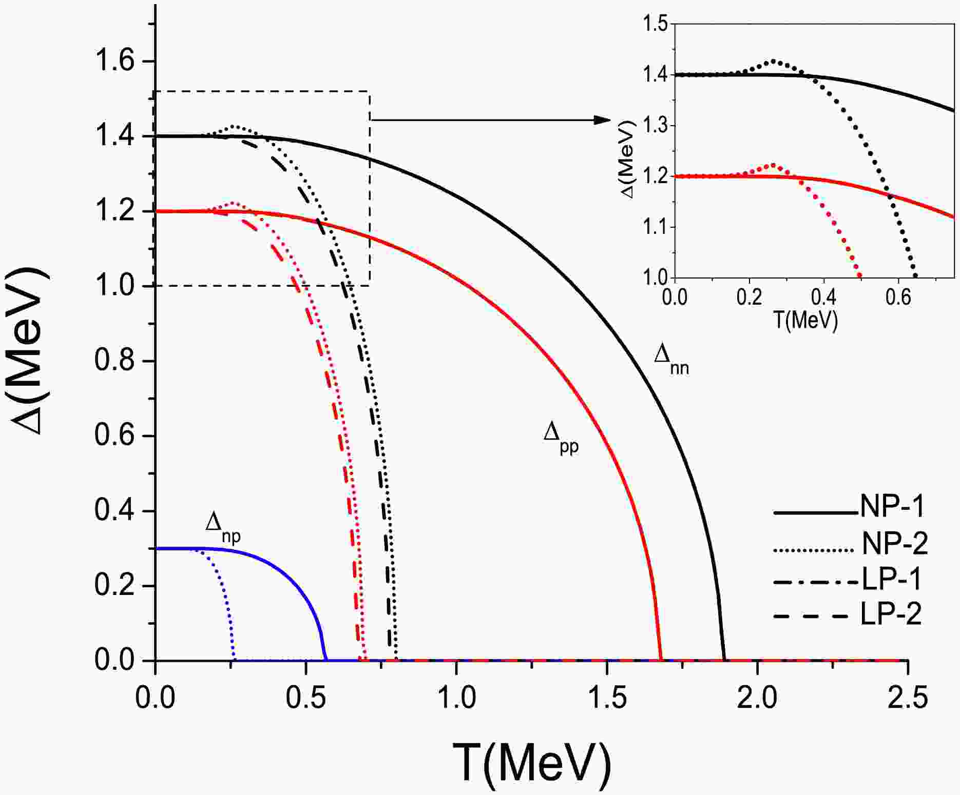
The variations in the various gap parameters as functions of the temperature are shown in Fig. 1. They are compared with the results obtained using the method described in Refs. [100−102] for isovector np pairing. In the following, the present method is designated by the abbreviation NP-1 and that of Refs. [100−102] by the abbreviation NP-2. The variations in
$ \Delta_{tt}(T) $ in the pairing between like-particles obtained using the method described in Ref. [104] (designated by the abbreviation LP-1) and the standard FTBCS method (designated by the abbreviation LP-2) are also reported in this figure.
Figure 1. (color online) Variations in the pairing gap parameters
$ \Delta_{nn} $ (black),$ \Delta_{pp} $ (red), and$ \Delta_{np} $ (blue) as functions of the temperature T within the framework of the Richardson model. Solid lines refer to the NP-1 model (present work), and dotted lines refer to the NP-2 model (Refs. [100−102]) for isovector pairing. Dash-dotted lines refer to the LP-1 model (Ref. [104]) and dashed lines refer to the LP-2 (standard FTBCS) model in pairing between like-particles. The$ \Delta_{nn} $ and$ \Delta_{pp} $ curves in NP-1 and LP-1 models are exactly superposed.Surprisingly, the
$ \Delta_{tt}\left( T\right) $ curves of this paper overlap with those of LP-1. We observe from the figure that the behavior of$ \Delta_{tt^{\prime}}(T) $ of this paper is similar to that of$ \Delta_{nn}\left( T\right) $ and$ \Delta_{pp}\left( T\right) $ in the standard FTBCS method (LP-2). We note in particular the existence of critical temperatures (which will be denoted as$ T_{ctt^{\prime}} $ ,$ t,t^{\prime}=n,p, $ in the following) beyond which the gap parameters vanish. However, their values are significantly higher than those obtained in both LP-2 and NP-2 methods. Therefore, the present model predicts the existence of an isovector pairing at temperatures beyond which the NP-2 model predicts. However, no exact values exist for isovector pairing as in like-particle pairing [107]. Therefore, we cannot decide between the two methods. However, NP-1 is a generalization of LP-1, whereas NP-2 is a generalization of LP-2 (FTBCS). LP-1 reproduces exact values better than LP-2 in a wider temperature range (see Ref. [104]). This may suggest that the NP-1 results would be better than those of NP-2.Moreover, in the present method, the curves of
$ \Delta_{nn}\left( T\right) $ and$ \Delta_{pp}\left( T\right) $ exhibit a plateau in the neighborhood of$ T_{cnp} $ , whereas in NP-2, they increase in the vicinity of$ T_{cnp} $ before decreasing from this value of T (see the enlarged part of Fig. 1). The NP-1 and NP-2 results differ significantly although the models are both developed within the path integral formalism because of the nature of the approximations used, which are different in the two models. -
For a comparison between the results of the various models, we consider the excitation energy
$E_{\rm exc}$ , defined as$ E_{\rm exc}\left( T\right) =E(T)-E(0), $

(47) rather than the energy of the system. The variations in
$E_{\rm exc}\left( T\right)$ are shown in Fig. 2 for the previously cited four models. The angular points that appear in each of these models correspond to the critical temperatures (see Fig. 1). Three appear in the isovector pairing case and two in the like-particles pairing case.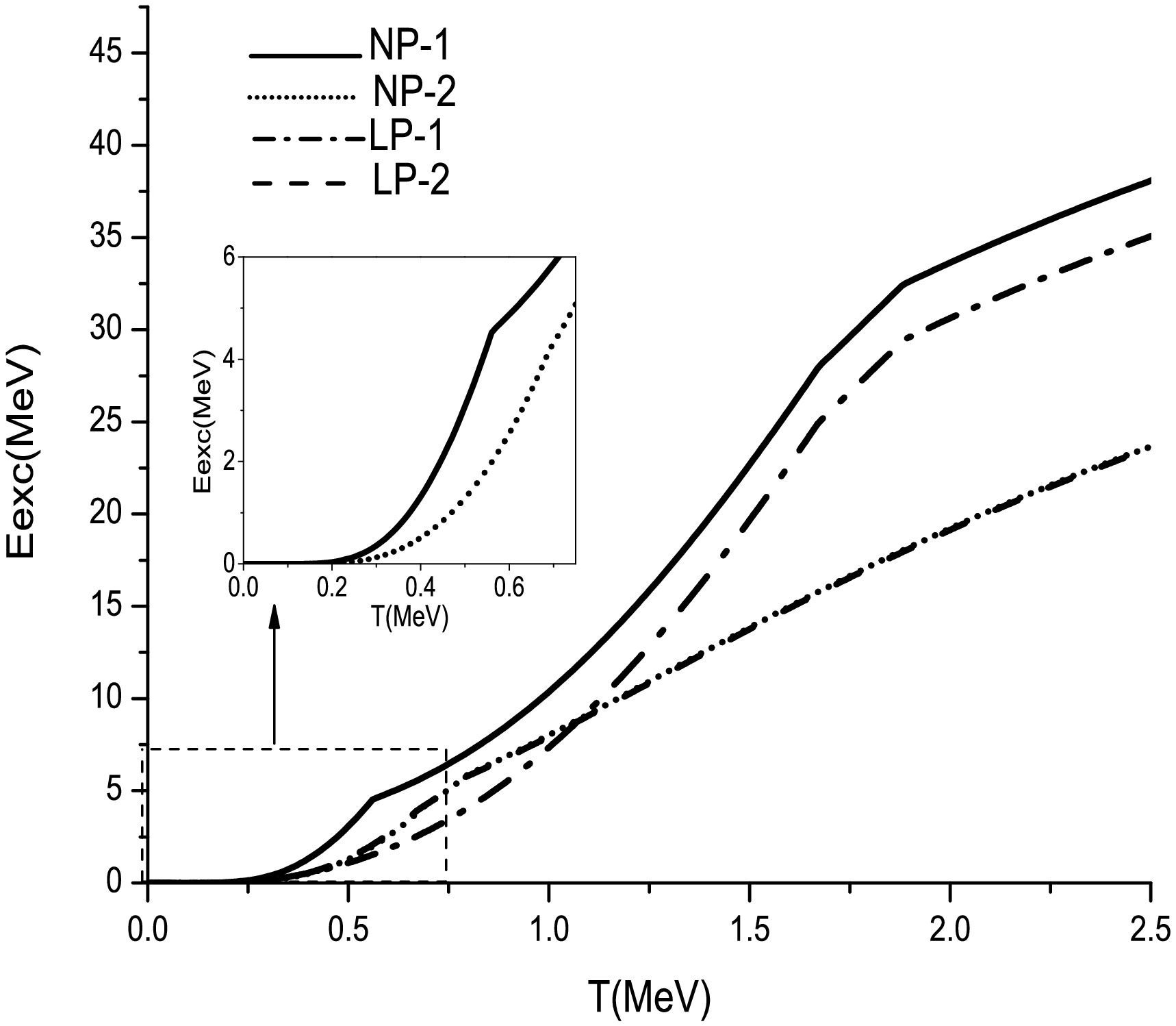
Figure 2. Variation in the excitation energy
$E_{\rm exc}\left( T\right)$ as a function of the temperature T within the framework of the Richardson model. Solid lines refer to the NP-1 model (present work) and dotted lines to the NP-2 model (Refs. [100−102]) for isovector pairing. Dash-dotted lines refer to the LP-1 model (Ref. [104]) and dashed lines refer to the LP-2 (standard FTBCS) model for pairing between like-particles.The figure shows that, for isovector pairing, when
$ T<\left( T_{cnp}\right) _{1}, $ the increase in$E_{\rm exc}$ is faster in the NP-1 model than in NP-2 model (see the enlarged part of Fig. 2). Moreover, we can evaluate the isovector pairing effect using the discrepancies$ \delta E_{{\rm exc}1}=E_{\rm exc}\left( NP\text-1\right) -E_{\rm exc}\left( LP\text-1\right) $

(48) and
$ \delta E_{{\rm exc}2}=E_{\rm exc}\left( NP\text-2\right) -E_{\rm exc}\left( LP\text-2\right) , $

(49) because the NP-1 (NP-2) model is a generalization of the LP-1 (LP-2) model.
$\delta E_{{\rm exc}1}$ is clearly more important than$\delta E_{{\rm exc}2}$ , which is very small. Indeed, the LP-2 and NP-2 graphs are very close to each other and appear superposed in the figure. This is because the$ \Delta_{pp}\left( T\right) $ and$ \Delta_{nn}\left( T\right) $ graphs are very close in these two approaches (see Fig. 1). In contrast,$\delta E_{{\rm exc}1}$ may reach up to$ 3 $ $\text {MeV}$ . Therefore, according to the present model, the isovector pairing effect on the excitation energy is more important than what the NP-2 model predicts.Beyond
$ T_{cnn} $ of the present model, all curves are parallel because no more pairing occurs in this region. However, in this temperature range, the graphs of$E_{\rm exc}\left( T\right)$ are not superposed because the$ E\left( 0\right) $ values are different in the various approaches. -
Next, we have studied the variation in the total heat capacity of the system C as a function of the temperature. The corresponding results are reported in Fig. 3 and compared with those obtained using the NP-1, LP-1, and LP-2 methods.
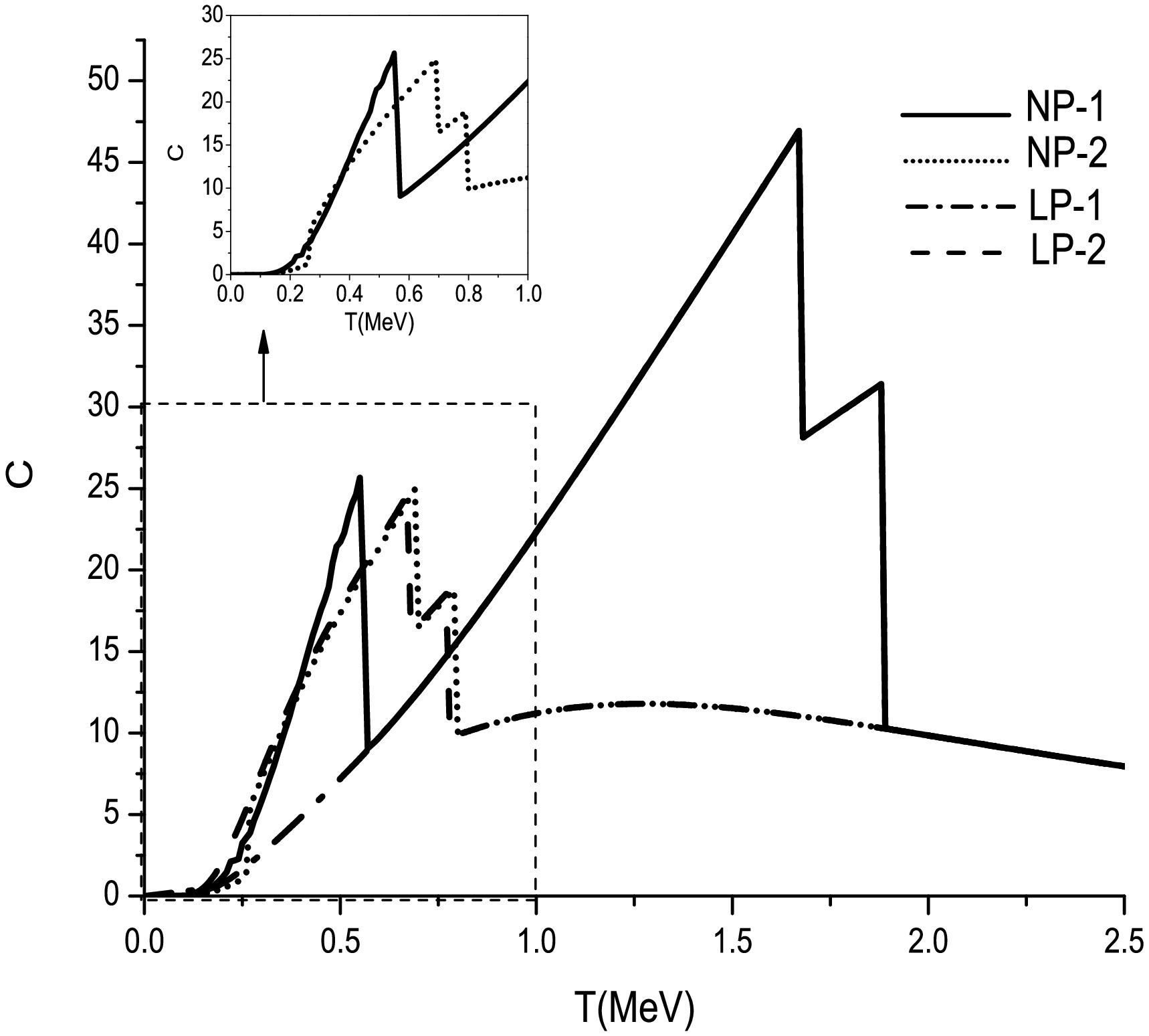
Figure 3. Variation in the heat capacity C as a function of the temperature T within the framework of the Richardson model. Solid lines refer to the NP-1 model (present work), and dotted lines refer to the NP-2 model (Refs. [100−102]) for isovector pairing. Dash-dotted lines refer to the LP-1 model (Ref. [104]) and dashed lines refer to the LP-2 (standard FTBCS) model in pairing between like-particles.
The figure shows that the overall behavior is similar for the four approaches: the peaks correspond to the various critical temperatures. The behavior of the pairing parameters is reflected in the heat capacity. Thus, the present method does not enable us to reproduce the S-shaped curve of the experimental heat capacities [108−110]. This is owing to the approximations used, namely, on the one hand, assuming that the different terms of the total Hamiltonian commute, and, on the other hand, the static-path and saddle-point approximations.
Similar to the excitation energy, the curves of heat capacity obtained using NP-2 and LP-2 are practically superposed, even if a slight shift occurs. Moreover, the peak corresponding to
$ \left( T_{cnp}\right) _{2} $ is barely visible (see the enlarged part of Fig. 3).We notice that the C values of this study are significantly higher than those predicted by the other methods. The values at
$ T=T_{ctt^{\prime}} $ are almost twice as large as in NP-2.Here again, the curves join beyond
$ T_{cnn} $ of the present method because no more pairing occurs in this region. -
In realistic cases, we used the single-particle energies of a Woods-Saxon deformed mean-field with the parameters described in Ref. [111], with a maximum number of shells of
$N_{\rm max}=12$ .In the following, we consider three nuclei as illustrative examples:
$^{36}{\rm Ar}$ ,$^{48}{\rm Cr}$ , and$^{64}{\rm Ge}$ . These nuclei are such that$ N=Z $ because the np pairing in this type of systems must be maximal. Moreover, for these nuclei, the pairing gap parameters$ \Delta_{tt^{\prime}}\left( 0\right) , $ $ t,t^{\prime}=n,p $ may be deduced from the even-odd mass differences. They are given by [12]$ \begin{aligned}[b] \Delta_{pp} =\;&-\frac{1}{8}[M(Z+2,N)-4M(Z+1,N)\\ & +6M(Z,N)-4M(Z-1,N)-4M(Z-2,N)] \end{aligned} $

(50) $ \begin{aligned}[b] \Delta_{nn} =\;&-\frac{1}{8}[M(Z,N+2)-4M(Z,N+1)\\ & +6M(Z,N)-4M(Z,N-1)-4M(Z,N-2)] \end{aligned} $

(51) $ \begin{aligned}[b] \Delta_{np} =\;&\frac{1}{4}\{2\left[ M(Z,N+1)+M(Z,N-1)\right. \\ & \left. +M(Z-1,N)+M(Z+1,N)\right] -4M(Z,N)\\ & -[M(Z+1,N+1)+M(Z-1,N+1)\\ & +M(Z+1,N-1)+M(Z+1,N-1)]\} \end{aligned} $

(52) where
$ M(Z,N) $ is the experimental mass value.Moreover, results concerning these nuclei obtained within the framework of the NP-2 method are available in Ref. [101]. However, the nuclei for which semiexperimental heat capacity data is available, such as
$^{162}{\rm Dy}$ and$^{172}{\rm Yb}$ , which were considered in Ref. [104], have a large$ (N-Z) $ value. In these nuclei, np pairing is negligible. -
The variations in
$ \Delta_{tt^{\prime}}\left( T\right) $ as functions of the temperature for these nuclei are shown in Figs. 4, 5, and 6 for the NP-1, NP-2, LP-1, and LP-2 approaches. Note that the values of NP-2 are extracted from Ref. [101], where the temperature values only go up to 2$\text {MeV}$ . Additionally, for the$^{36}{\rm Ar}$ and$^{64}{\rm Ge}$ nuclei, the "experimental" values of$ \Delta_{tt^{\prime}}\left( 0\right) $ are less well reproduced for the NP-2 model than the NP-1 model.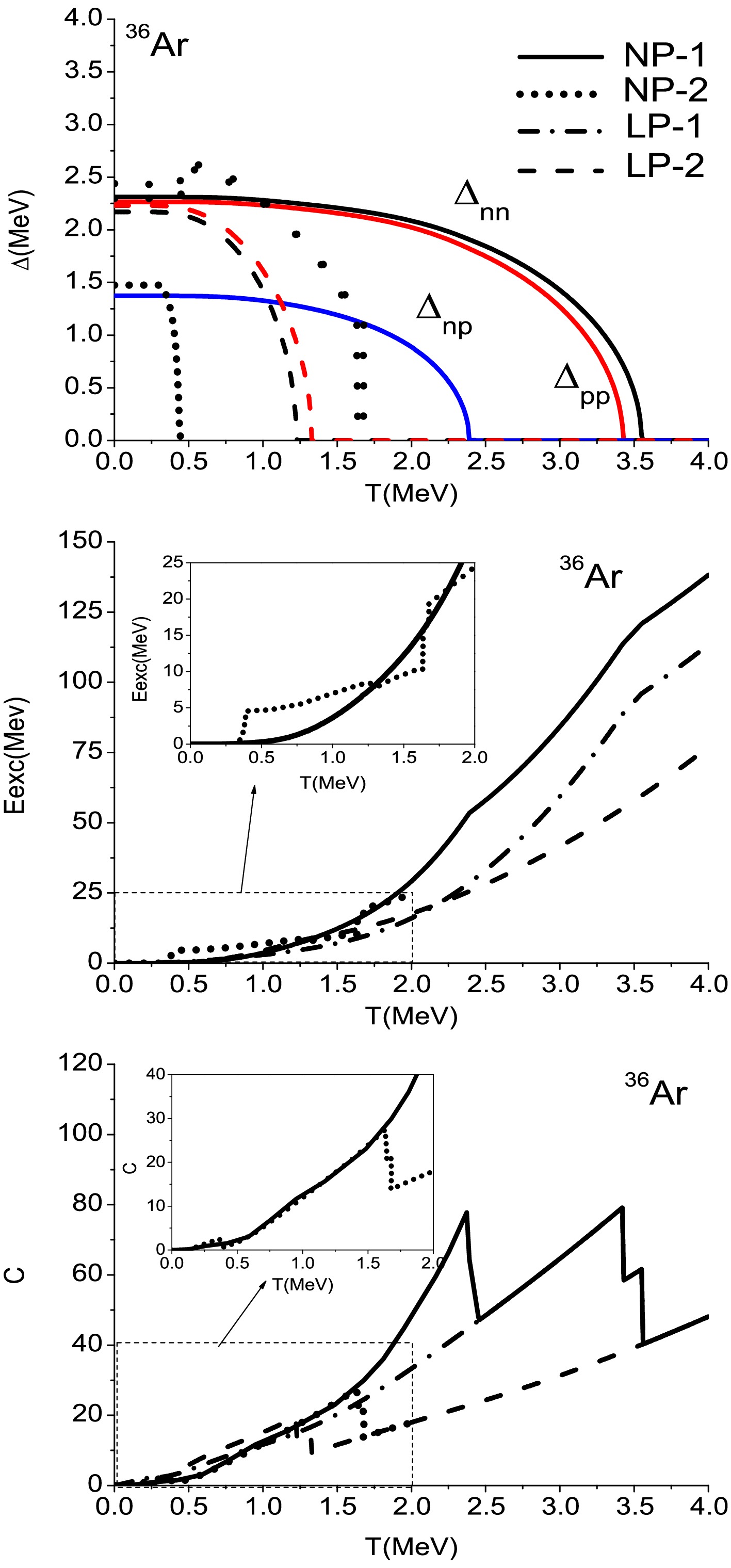
Figure 4. (color online) Variations in the pairing gap parameters
$ \Delta_{tt^{\prime}}\left( T\right) $ ,$ t,t^{\prime}=n,p $ (upper part), excitation energy$E_{\rm exc}$ (middle), and heat capacity C as functions of the temperature T for the nucleus$^{36}{\rm Ar}$ . Solid lines refer to the NP-1 model (present work), dotted lines refer to the NP-2 model (Refs. [100−102]) for isovector pairing. Dash-dotted lines refer to the LP-1 model (Ref. [104]) and dashed lines refer to the LP-2 (standard FTBCS) model for pairing between like-particles. The$ \Delta_{nn} $ and$ \Delta_{pp} $ curves in the NP-1 and LP-1 models are exactly superposed.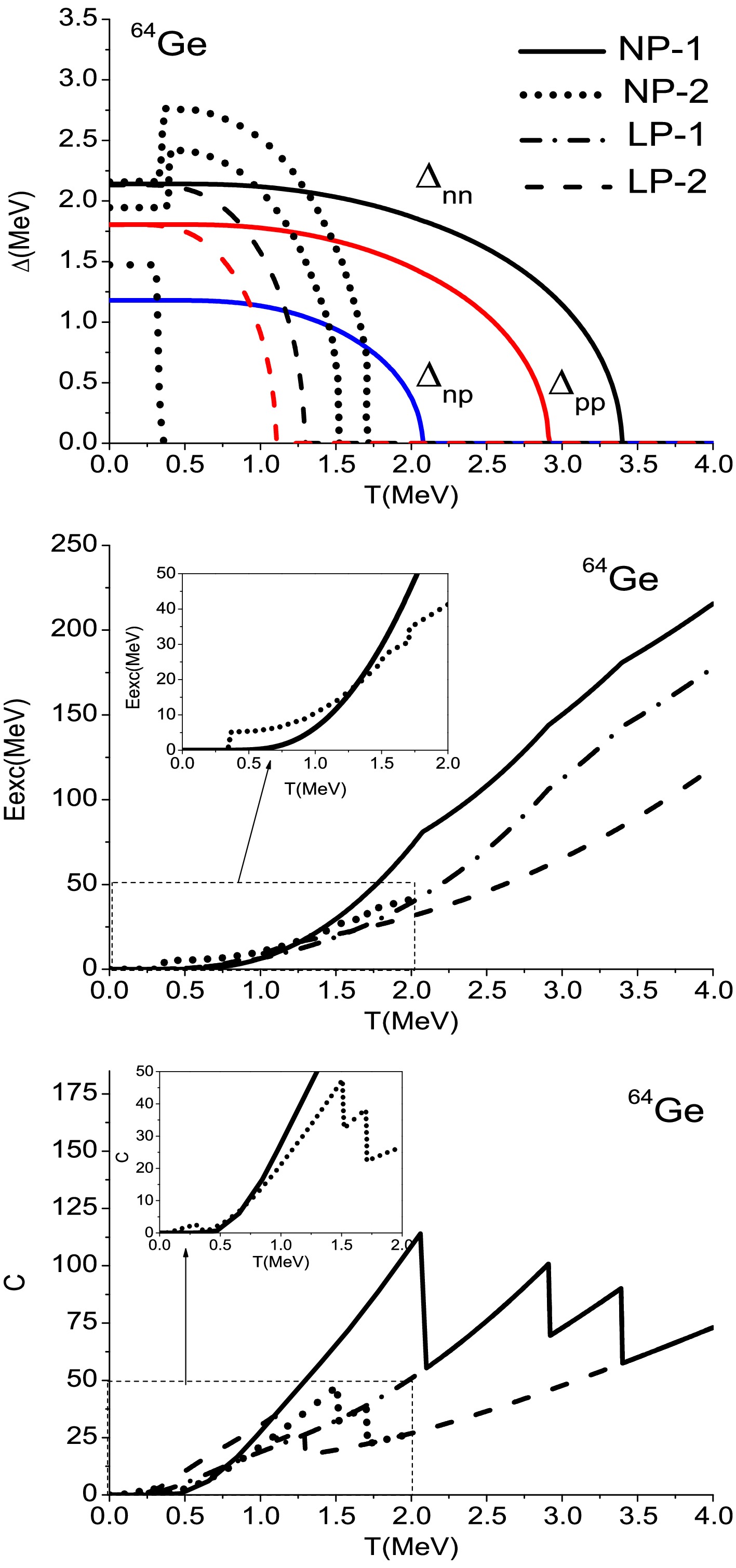
Figure 6. (color online) Same as Fig. 4 for the nucleus
$^{64}{\rm Ge}$ .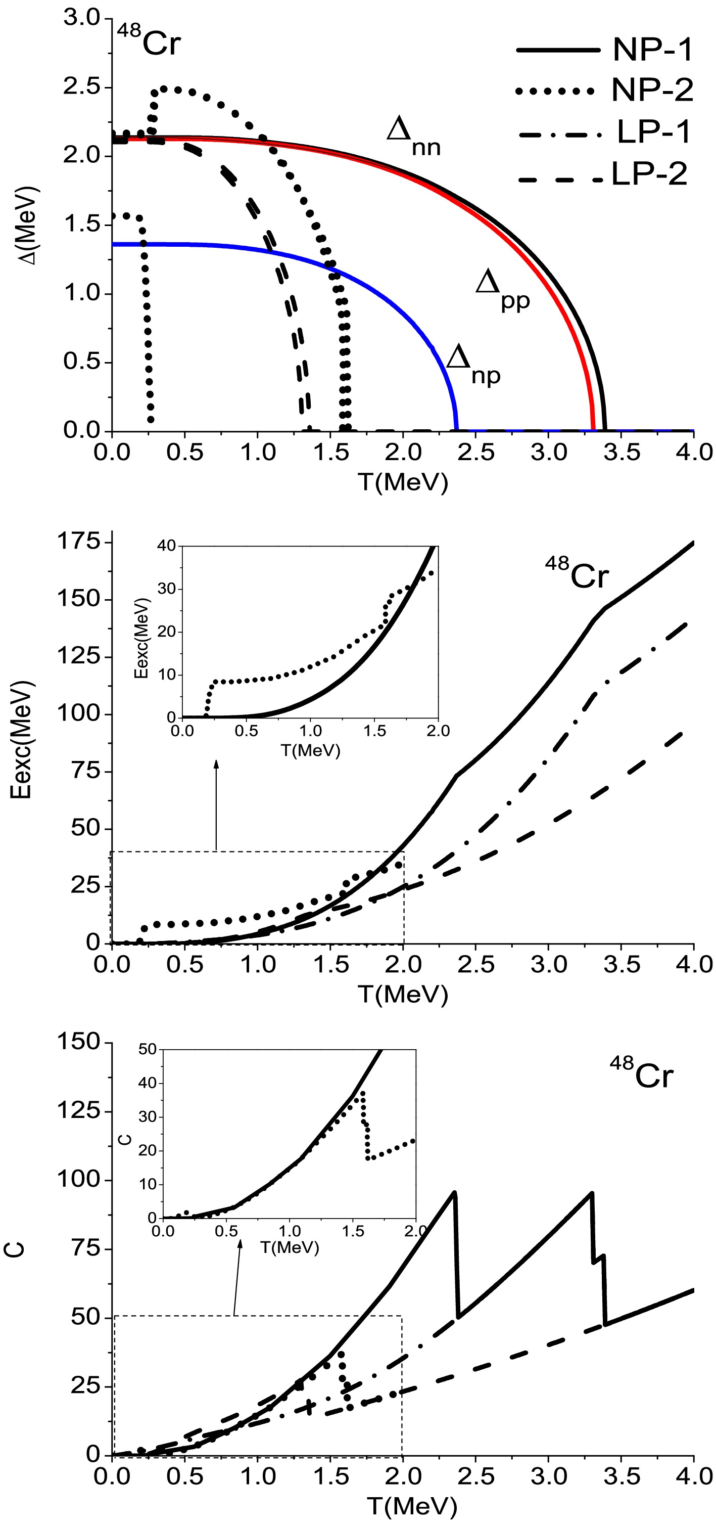
Figure 5. (color online) Same as Fig. 4 for the nucleus
$^{48}{\rm Cr}$ .For the three considered nuclei, the
$ \Delta_{tt}\left( T\right) $ of the NP-1 and LP-1 methods overlap, similar to the schematic case. We have not found an explanation for this fact.Moreover, the overall behavior of the three gap parameters of the present method is similar to that of the standard FTBCS method (LP-2). The abrupt increase in the
$ \Delta_{nn} $ and$ \Delta_{pp} $ curves and abrupt decrease in the$ \Delta_{np} $ curve at$ T=T_{cnp} $ that appear in NP-2 method no longer exist in NP-1.Moreover, the critical temperatures of the present model are clearly more important than the ones predicted by NP-2 and LP-2 methods. Their values are more than twice those predicted by the NP-2 and LP-2 models.
-
The variations in
$E_{\rm exc}\left( T\right)$ as functions of the temperature are reported in the same figure as$ \Delta_{tt^{\prime}} $ for each of the considered nuclei. We can observe a change in the slope of$E_{\rm exc}$ at the various critical temperatures. However, the change in the isovector pairing case is less sudden within the framework of NP-1 model than within the NP-2 one. This is a direct consequence of the behavior of$ \Delta_{tt^{\prime} }\left( T\right) $ .For all the considered nuclei, the excitation energy of NP-2 model increases faster than that of NP-1, until
$ T=T_{cnn} $ of NP-2 model. Beyond this value, the result is inverted.We have evaluated the isovector pairing effect on the excitation energy using the quantities
$\delta E_{{\rm exc}1}$ and$\delta E_{{\rm exc}2}$ defined by Eqs. (48) and (49). Their respective values at$ T=\left( T_{cnp}\right) _{1} $ and$ T=\left( T_{cnp}\right) _{2} $ are given in Table 1. The np pairing contribution to the excitation energy appears to be much more important in the framework of the NP-1 model than in the NP-2 model.Nucleus $\delta E_{ {\rm exc}1}( ( T_{cnp}) _{1}) /\rm MeV$ 

$\delta E_{{\rm exc}2}( ( T_{cnp}) _{2}) /\rm MeV$ 

$^{36}{\rm Ar}$ 

24.86 2.51 $^{48}{\rm Cr}$ 

32.76 8.46 $^{64}{\rm Ge}$ 

37.76 5.06 Table 1. Isovector pairing effect on the excitation energy evaluated at the neutron-proton critical value of the temperature (see the text for notations).
When
$ T>T_{cnn} $ of the NP-1 model, all curves are parallel because no more pairing occurs in this region. Nevertheless, as in the schematic case, the excitation energy graphs are not superposed because the energy values at zero temperature are different in the various approaches. -
The variations in
$ C\left( T\right) $ as functions of the temperature are shown in Figs. 4−6. As in the schematic case, the overall behavior is similar for the four approaches: none of them can reproduce the S-shaped curve of the experimental heat capacities.For
$^{36}{\rm Ar}$ and$^{48}{\rm Cr}$ , the "experimental" values of$ \Delta _{nn}\left( 0\right) $ and$ \Delta_{pp}\left( 0\right) $ are very close to each other. The$ \Delta_{tt}\left( T\right) $ ,$ t=,np, $ curves are then practically superposed in all the models. Thus, the peaks in the$ C\left( T\right) $ curves at$ T_{cnn} $ and$ T_{cpp} $ are very close and, in some cases, difficult to distinguish.A shift exists between the peaks positions at
$ T=T_{cnn} $ and$ T=T_{cpp} $ between the NP-2 and LP-2 models. This is due to the shift observed in the$ \Delta_{tt}\left( T\right) $ graphs between these two models. This shift does not exist between the NP-1 and LP-1 approaches: the$ C(T) $ curves are exactly superposed when$ T>\left( T_{cnp}\right) _{1} $ .In the isovector pairing case, the height of the peak in NP-2 approach at
$ T=\left( T_{cnp}\right) _{2} $ is small compared with the peaks corresponding to the proton and neutron critical temperature values. However, the peak in NP-1 at$ T=\left( T_{cnp}\right) _{1} $ is comparable to that of its homologues at$ T=T_{cnn} $ and$ T=T_{cpp} $ . Moreover, the peak at$ T=\left( T_{cnp}\right) _{2} $ is negligible compared with the one at$ T=\left( T_{cnp}\right) _{1} $ .In the temperature range between
$ \left( T_{cnp}\right) _{2} $ and$ T_{cpp} $ of the NP-2 aproach, the NP-1 and NP-2 curves are very close to each other for the nuclei$ ^{36}Ar $ and$ ^{48}Cr $ . The discrepancy observed for$ ^{64}Ge $ is probably due to the$ \Delta_{tt^{\prime}}\left( 0\right) $ ,$ t,t^{\prime}=n,p $ values being different in the two models.All the curves for the four considered models join when
$ T>T_{cnn} $ of model NP-1, because no more pairing occurs in this region.In summary, the main conclusions drawn in the schematic case remain valid in the realistic case.
However, the predicted critical temperatures appear to be too high. For pairing between like-particles, Ref. [104] showed that the LP-1 approach reproduces the exact results of the gap parameter, energy, and heat capacity at low temperatures well. However, this is no longer the case at higher temperatures. This leads to an overestimation of the energy values for higher temperatures.
As the NP-1 approach is a generalization of LP-1, we can assume that
$ \Delta_{tt\prime} $ ,$ {t,t\prime=n,p} $ ,$E_{\rm exc}$ , and C are correctly described by the NP-1 approach at low temperatures. However, the latter appears to overestimate the critical temperatures, which leads to excessive values of$E_{\rm exc}$ . To solve this problem, we should consider the thermal and quantal fluctuations and perform a particle-number projection. -
We present a model for the treatment of the temperature dependent np pairing correlations based on the path integral formalism (model NP-1). It generalizes the recently proposed model using a similar approach in the pairing between like-particles (model LP-1).
The pairing terms in the total Hamiltonian are expressed in a square form to facilitate the use of the Hubbard-Stratonovitch transformation. The expression for the partition function of the system is then established using the static path approximation.
The gap equations, as well as the expressions for the energy, entropy, and heat capacity of the system are deduced. They generalize those of the LP-1 model. We simply must set
$ \Delta_{np}=0 $ in the expressions of NP-1 model to determine the equations of the LP-1 model. Moreover, they are different from the ones obtained using the NP-2 model (which is a generalization of the standard FTBCS model LP-2) because the approximations used are of a different nature.As a first step, the formalism is numerically applied within the framework of the schematic Richardson model. The method is then applied to realistic cases using the single-particle energies of a deformed Woods-Saxon mean-field. Three nuclei with
$ N=Z $ are considered becausethe np pairing must be maximal in this type of systems: $^{36}{\rm Ar}$ ,$^{48}{\rm Cr}$ , and$^{64}{\rm Ge}$ .The variations in the three gap parameters, excitation energy, and heat capacity are studied as functions of the temperature in both schematic and realistic cases. They are compared with the results of the LP-1, NP-2, and LP-2 approaches. The conclusions in the schematic and realistic cases are similar.
We observe that the behavior of the three gap parameters of NP-1 model is similar to that of
$ \Delta_{tt}\left( T\right) $ in the standard FTBCS model. Critical values of the temperature exist beyond which$ \Delta_{tt^{\prime}} $ ...$ t,t^{\prime}=n,p $ ,vanish. These critical temperatures are significantly larger in the NP-1 and LP-1 models than in the NP-2 and LP-2 models. Moreover, the$ \Delta_{tt}\left( T\right) , $ of the NP-1 and LP-1 models are exactly superposed, whereas those of the NP-2 and LP-2 models are different. Furthermore, the sudden variation in the graphs of$ \Delta _{tt}\left( T\right) $ in the vicinity of$ T_{cnp} $ in the NP-2 model no longer exists in the NP-1 model.T
he isovector np pairing contribution to the excitation energy predicted using the NP-1 model appears to be more important than the one predicted by NP-2 model. Finally, the heat capacity exhibits an overall behavior that is similar in the four approaches: none of them can reproduce the S-shaped curve of the experimental heat capacities. Each model has a peak at each value of the critical temperature. These peaks are significantly higher in the framework of the NP-1 and LP-1 models than in the framework of the NP-2 and LP-2 models.
However, note that no experimental data are available for the considered nuclei. Therefore, deciding between the different approaches is difficult. Nevertheless, the model NP-1 appears to overestimate the critical temperatures. To remedy this problem, we should consider the thermal and quantal fluctuations and perform a particle-number projection.
It would also be interesting to generalize the present study to the isovector plus isoscalar pairing case.
-
Let us consider the unitary operator
$ U_{np}=U_{n}U_{p} $

(A1) with
$ U_{t}=\prod\limits_{j>0}\mathcal{S}_{jt}\text{ , }\mathcal{S}_{jt}={\rm i}\left( a_{jt}+a_{jt}^+\right) \left( a_{\tilde{j}t}+a_{\tilde{j}t} ^+\right) \text{, }t=n,p. $

(A2) We can easily verify that
$ U_{np}^+=U_{np}. $

(A3) The operators
$ P_{np}^{+}U_{np} $ and$ U_{np}^{+}P_{np} $ are identical and are given by$ P_{np}^+U_{np}=U_{np}^+P_{np}=R_{np} $

(A4) where
$ R_{np}=\sum\limits_{\nu>0}\left[ \eta_{\nu n}\eta_{\tilde{\nu}p}B_{\nu n\tilde{p}}+\eta_{\nu p}\eta_{\tilde{\nu}n}B_{\nu p\tilde{n} }\right] $

(A5) with
$ \begin{align} B_{\nu n\tilde{p}} & =\left( a_{\tilde{\nu}n}+a_{\tilde{\nu} n}^+\right) \left( a_{\nu p}+a_{\nu p}^+\right) \prod \limits_{\substack{j>0\\j\neq\nu}}\mathcal{S}_{jn}\text{ }\mathcal{S}_{jp} \end{align} $

(A6) $ \begin{align} B_{\nu p\tilde{n}} & =\left( a_{\tilde{\nu}p}+a_{\tilde{\nu} p}^+\right) \left( a_{\nu n}+a_{\nu n}^+\right) \prod \limits_{\substack{j>0\\j\neq\nu}}\mathcal{S}_{jn}\text{ }\mathcal{S}_{jp}. \end{align} $

(A7) Finally, we have
$ P_{np}^+P_{np}=P_{np}^+U_{np}U_{np}^+P_{np}=R_{np}^{2}. $

(A8) -
Let us set in Eq. (8)
$ \begin{aligned}[b] \mathsf{S}_{tt^{\prime}}\left( \beta\right) & =T_{\tau}\text{ }\exp\left( \int_{0}^{\beta}H_{tt^{\prime}}\left( \tau\right) {\rm d}\tau\right) \\ & =\underset{N\rightarrow \infty}{\lim}T_{\tau}\prod\limits_{i=1}^{N} \exp\left( \frac{\beta}{N}H_{tt^{\prime}}\left( \tau_{i}\right) \right) \text{ , }t,t^{\prime}=n,p. \end{aligned} $

(B1) We then have
$ \mathsf{S}\left( \beta\right) =\mathsf{S}_{nn}\left( \beta\right) \mathsf{S}_{pp}\left( \beta\right) \mathsf{S}_{np}\left( \beta\right) . $

(B2) Using the Hubbard-Stratonovitch transformation [91, 112, 113]
$ \exp\left( O^{2}\right) =\int\nolimits_{-\infty}^{+\infty}{\rm d}x\exp\left\{ -\pi x^{2}-2\sqrt{\pi}xO\right\} ,$

(B3) where O is a bounded Hermitian operator and x is an external field; the quantities
$ \mathsf{S}_{tt^{\prime}}\left( \beta\right) $ , become$ \begin{aligned}[b] \mathsf{S}_{tt^{\prime}}\left( \beta\right) =\;&T_{\tau}\underset {N\rightarrow \infty}{\lim}\prod\limits_{i=1}^{N}\int\nolimits_{-\infty }^{+\infty}\sqrt{\frac{\beta}{N}}{\rm d}X_{tt^{\prime}i}\exp\left\{ -\pi\frac {\beta}{N}X_{tt^{\prime}i}^{2}\right. \\& \left. -2\frac{\beta}{N}\sqrt{\pi G_{tt^{\prime}}}X_{tt^{\prime} i}R_{tt^{\prime}}\left( \tau_{i}\right) \right\} \end{aligned} $

(B4) where we set, for simplicity
$ x_{tt^{\prime}i}=x_{tt^{\prime}}\left( \tau_{i}\right) ,$

(B5) and
$ X_{tt^{\prime}i} $ is such that$ x_{tt^{\prime}i}=\sqrt{\frac{\beta}{N}}X_{tt^{\prime}i}. $

(B6) At the limit where N goes to infinity, we set
$ \int\mathfrak{D}X_{tt^{\prime}}=\underset{N\rightarrow \infty}{\lim} \int_{-\infty}^{+\infty}\prod\limits_{j=1}^{N}\sqrt{\frac{\beta}{N} }{\rm d}X_{tt^{\prime}j}. $

(B7) Note that
$ X_{tt^{\prime}j} $ here means$ X_{tt^{\prime} }\left( \tau_{j}\right) $ and when the limit is taken,$ X_{tt^{\prime }j}\rightarrow X_{tt^{\prime}}\left( \tau\right) $ .$ \mathsf{S}_{tt^{\prime}}\left( \beta\right) $ finally reads$ \begin{aligned}[b] S_{tt^{\prime}}\left( \beta\right) =\;&T_{\tau}\int\mathfrak{D}X_{tt^{\prime} }\exp\left\{ -\pi\int\nolimits_{0}^{\beta}X_{tt^{\prime}}^{2}\left( \tau\right) {\rm d}\tau\right. \\& \left. -2\sqrt{\pi G_{tt^{\prime}}}\int\nolimits_{0}^{\beta}R_{tt^{\prime} }\left( \tau\right) X_{tt^{\prime}}\left( \tau\right) {\rm d}\tau\right\} . \end{aligned} $

(B8) Let us set
$ \Delta_{tt^{\prime}}\left( \tau\right) =\sqrt{\pi G_{tt^{\prime}} }X_{tt^{\prime}}\left( \tau\right) , $

(B9) the partition function Z is then given by
$ \begin{aligned}[b] Z =\;&T_{\tau}Tr\int \mathfrak{D}\Delta_{nn}\mathfrak{D}\Delta_{pp}\mathfrak{D}\Delta_{np} \\&\times\exp\left\{ -\int\nolimits_{0}^{\beta}\left[ \frac{\Delta_{nn}^{2}\left( \tau\right) }{G_{nn}}+\frac{\Delta_{pp}^{2}\left( \tau\right) }{G_{pp} }+\frac{\Delta_{np}^{2}\left( \tau\right) }{G_{np}}\right] {\rm d}\tau\right\} \\ & \times\exp\Bigg\{ -\beta H_{0}-2\int\nolimits_{0}^{\beta}\Big[ R_{nn}\left( \tau\right) \Delta_{nn}\left( \tau\right) +R_{pp}\left( \tau\right) \Delta_{pp}\left( \tau\right) \\& +R_{np}\left( \tau\right) \Delta_{np}\left( \tau\right) \Big] {\rm d}\tau\Bigg\}, \end{aligned} $

(B10) where
$ \int\mathfrak{D}\Delta_{tt^{\prime}}=\underset{N\rightarrow \infty}{\lim} \int_{-\infty}^{+\infty}\prod\limits_{j=1}^{N}\sqrt{\frac{\beta}{N}}\frac {1}{\sqrt{\pi G_{tt^{\prime}}}}{\rm d}\Delta_{tt^{\prime}j}. $

(B11) Using the static-path approximation [114], where we assume that
$ \Delta_{tt^{\prime}}\left( \tau\right) $ is independent of τ, i.e.,$ \Delta_{tt^{\prime}}\left( \tau\right) =\Delta_{tt^{\prime}}, $

(B12) Z reduces to ordinary integrals over the variables
$ \Delta_{tt^{\prime}}. $ It then reads as$ \begin{aligned}[b] Z =\;&\frac{1}{\pi^{3/2}\sqrt{G_{nn}G_{pp}G_{np}}}\int {\rm d}\Delta_{nn} {\rm d}\Delta_{pp}{\rm d}\Delta_{np}\\&\times\exp\left\{ -\beta\left[ \frac{\left\vert \Delta_{nn}\right\vert ^{2}}{G_{nn}}+\frac{\left\vert \Delta_{pp}\right\vert ^{2} }{G_{pp}}+\frac{\left\vert \Delta_{np}\right\vert ^{2}}{G_{np}}\right] \right\} {\rm Tr}\\&\times\exp\left( -\beta\sum\limits_{\nu}h_{\nu np}\right) \end{aligned} $

(B13) with
$ \begin{aligned}[b] h_{\nu np} =\;&\tilde{\varepsilon}_{\nu n}\left( \eta_{\nu n} +\eta_{\tilde{\nu}n}\right) +\tilde{\varepsilon}_{\nu p}\left( \eta_{\nu p}+\eta_{\tilde{\nu}p}\right) +2\Delta_{nn}\eta_{\nu n} \eta_{\tilde{\nu}n}B_{\nu n}\\&+2\Delta_{pp}\eta_{\nu p}\eta_{\tilde{\nu }p}B_{\nu p} +2\Delta_{np}\left( \eta_{\nu n}\eta_{\tilde{\nu}p}B_{\nu n\tilde{p}}+\eta_{\tilde{\nu}n}\eta_{\nu p}B_{\nu p\tilde{n} }\right) \end{aligned} $

(B14) -
Let us set
$ h_{\nu np}=\sum\limits_{t}h_{\nu t}+h_{\nu np}^{\prime} $

(C1) with
$ h_{\nu t}=\tilde{\varepsilon}_{\nu t}\left( \eta_{\nu t}+\eta _{\tilde{\nu}t}\right) +2\Delta_{tt}\eta_{\nu t}\eta_{\tilde{\nu} t}B_{\nu t} $

(C2) and
$ h_{\nu np}^{\prime}=2\Delta_{np}\left( \eta_{\nu n}\eta_{\tilde{\nu} p}B_{\nu n\tilde{p}}+\eta_{\tilde{\nu}n}\eta_{\nu p}B_{\nu p\tilde{n}}\right) . $

(C3) The commutation relation between
$ h_{\nu np} $ and$ h_{\mu np} $ is given by$ \begin{aligned}[b] \left[ h_{\nu np},h_{\mu np}\right] =\;&\sum_{tt^{\prime}}\left[ h_{\nu t},h_{\mu t^{\prime}}\right] +\sum_{t}\left[ h_{\nu t},h_{\mu np}^{\prime }\right] \\ & +\sum_{t}\left[ h_{\nu np}^{\prime},h_{\mu t}\right] +\left[ h_{\nu np}^{\prime},h_{\mu np}^{\prime}\right] . \end{aligned} $

(C4) We then have
$ \begin{aligned}[b] \left[ h_{\nu t},h_{\mu t^{\prime}}\right] =\;&2\Delta_{t^{\prime} t^{\prime}}\tilde{\varepsilon}_{\nu t}\left[ \left( \eta_{\nu t} +\eta_{\tilde{\nu}t}\right) ,\eta_{\mu t^{\prime}}\eta_{\tilde{\mu }t^{\prime}}B_{\mu t^{\prime}}\right] \\ & +2\Delta_{tt}\tilde{\varepsilon}_{\mu t^{\prime}}\left[ \eta_{\nu t}\eta_{\tilde{\nu}t}B_{\nu t},\left( \eta_{\mu t^{\prime}} +\eta_{\tilde{\mu}t^{\prime}}\right) \right] \\ & +4\Delta_{tt}\Delta_{t^{\prime}t^{\prime}}\left[ \eta_{\nu t} \eta_{\tilde{\nu}t}B_{\nu t},\eta_{\mu t^{\prime}}\eta_{\tilde{\mu }t^{\prime}}B_{\mu t^{\prime}}\right] . \end{aligned} $

(C5) The first two terms in
$ \left[ h_{\nu t},h_{\mu t^{\prime}}\right] $ for$ \nu\neq\mu $ are proportional to$ \Delta_{t^{\prime}t^{\prime}} $ (and thus to$ \sqrt{G_{t^{\prime}t^{\prime}}} $ ) or to$ \Delta_{tt} $ (and thus to$ \sqrt{G_{tt}} $ ). The last term is proportional to the product$ \Delta_{tt}\Delta_{t^{\prime}t^{\prime}} $ (and thus to$ \sqrt{G_{tt} G_{t^{\prime}t^{\prime}}} $ ).Similarly,
$ \left[ h_{\nu t},h_{\mu np}^{\prime}\right] $ and$ \left[ h_{\nu np}^{\prime},h_{\mu t}\right] $ for$ \nu\neq\mu $ are the sum of a term proportional to$ \Delta_{np} $ (and thus to$ \sqrt{G_{np}} $ ) and another proportional to$ \Delta_{tt}\Delta_{np} $ (and thus to$ \sqrt{G_{tt}G_{np} } $ ). For example,$ \begin{aligned}[b] \left[ h_{\nu t},h_{\mu np}^{\prime}\right] =\;&2\Delta_{np}\\& \times\left[ \tilde{\varepsilon}_{\nu t}\left( \eta_{\nu t} +\eta_{\tilde{\nu}t}\right) ,\left( \eta_{\mu n}\eta_{\tilde{\mu} p}B_{\mu n\tilde{p}}+\eta_{\tilde{\mu}n}\eta_{\mu p}B_{\mu p\tilde{n}}\right) \right] \\& +4\Delta_{tt}\Delta_{np}\big[ \left( \eta_{\nu t}\eta_{\tilde{\nu} t}B_{\nu t}\right) ,\big( \eta_{\mu n}\eta_{\tilde{\mu}p}B_{\mu n\tilde{p}}\\&+\eta_{\tilde{\mu}n}\eta_{\mu p}B_{\mu p\tilde{n} }\big) \big] . \end{aligned} $

(C6) Finally,
$ \left[ h_{\nu np}^{\prime},h_{\mu np}^{\prime}\right] $ for$ \nu\neq\mu $ is proportional to$ \Delta_{np}^{2} $ (and thus to$ G_{np} $ ). As the values of$ G_{tt^{\prime}} $ ($ t,t^{\prime}=n,p $ ) are small compared with single-particle energies, the approximation$ \left[ h_{\nu np},h_{\mu np}\right] =0\text{ , }\nu\neq\mu, $

is justified.
-
The temperature dependent gap equations in the isovector pairing case of Ref. [100] are briefly recalled in the following.
The gap parameters
$ \Delta_{tt^{\prime}} $ $ \left( t,t^{\prime}=n,p\right) $ are defined by$ \begin{aligned}[b] \frac{4\Delta_{nn}}{G_{nn}}=\;&\sum_{\nu,\text{ }\tau=1,2}\frac{1}{E_{\nu\tau} }\tanh\frac{1}{2}\beta E_{\nu\tau}\Bigg\{ \Delta_{nn} +\frac{\left( -1\right) ^{\tau+1}}{R_{\nu}} \\ &\times \left[ \left( E_{\nu n}^{2}-E_{\nu p}^{2}\right) \Delta_{nn}+2\Delta_{np}^{2}\left( \Delta _{nn}+\Delta_{pp}\right) \right] \Bigg\} \end{aligned} $

(D1) $ \begin{aligned}[b] \frac{4\Delta_{pp}}{G_{pp}}=\;&\sum_{\nu,\text{ }\tau=1,2}\frac{1}{E_{\nu\tau} }\tanh\frac{1}{2}\beta E_{\nu\tau}\Bigg\{ \Delta_{pp} +\frac{\left( -1\right) ^{\tau+1}}{R_{\nu}} \\& \left[ \left( E_{\nu p}^{2}-E_{\nu n}^{2}\right) \Delta_{pp}+2\Delta_{np}^{2}\left( \Delta _{nn}+\Delta_{pp}\right) \right] \Bigg\} \end{aligned} $

(D2) $ \begin{aligned}[b] \frac{2}{G_{np}}=\;&\sum_{\nu,\text{ }\tau=1,2}\frac{1}{E_{\nu\tau}}\tanh\frac {1}{2}\beta E_{\nu\tau}\times\Bigg\{ 1+\frac{\left( -1\right) ^{\tau+1}}{R_{\nu}}\\ &\left[ E_{\nu n}^{2}+E_{\nu p}^{2}+2\left( \Delta_{nn}\Delta_{pp}-\tilde{\varepsilon }_{\nu n}\tilde{\varepsilon}_{\nu p}\right) \right] \Bigg\} . \end{aligned} $

(D3) with the notations
$ E_{\nu\tau}^{2}=\frac{1}{2}\left\{ E_{\nu n}^{2}+E_{\nu p}^{2}+2\Delta _{np}^{2}+\left( -1\right) ^{\tau+1}R_{\nu}\right\} \text{ , }\tau=1,2 $

(D4) $ R_{\nu}^{2}=\left( E_{\nu n}^{2}-E_{\nu p}^{2}\right) ^{2}+4\Delta_{np} ^{2}\left[ \left( \tilde{\varepsilon}_{\nu n}-\tilde{\varepsilon }_{\nu p}\right) ^{2}+\left( \Delta_{nn}+\Delta_{pp}\right) ^{2}\right] $

(D5) and
$ E_{\nu t}=\sqrt{\tilde{\varepsilon}_{\nu t}^{2}+\Delta_{tt}^{2}}. $

(D6) The particle-number conservation conditions are given by
$ N_{t}=\sum\limits_{\nu}\left\{ 1+\sum\limits_{\tau=1,2}\frac{\partial E_{\nu\tau}} {\partial\lambda_{t}}\tanh\frac{1}{2}\beta E_{\nu\tau}\right\} $

(D7) with
$ \begin{aligned}[b] \frac{\partial E_{\nu\tau}}{\partial\lambda_{n(p)}}=\;&\frac{1}{2E_{\nu\tau} }\Bigg\{ -\tilde{\varepsilon}_{\nu n(p)}+\left( -1\right) ^{\tau +1}\frac{1}{R_{\nu}} \\ & \times\left[ \tilde{\varepsilon}_{\nu n(p)}\left( E_{\nu p(n)}^{2}-E_{\nu n(p)}^{2}\right) +2\Delta_{np}^{2}\left( \tilde {\varepsilon}_{\nu p(n)}-\tilde{\varepsilon}_{\nu n(p)}\right) \right] \Bigg\} . \end{aligned} $

(D8) At the limit when
$ \Delta_{np}=0, $ Eqs. (D1) and (D2) become$ \frac{2}{G_{tt}}=\sum\limits_{\nu}\frac{1}{E_{\nu t}}\tanh\left( \frac{\beta }{2}E_{\nu t}\right) $

(D9) and the particle-number conservation conditions (87) become
$ N_{t}=\sum\limits_{\nu}\left[ 1-\frac{\tilde{\varepsilon}_{\nu t}}{E_{\nu t}}\tanh\left( \frac{\beta}{2}E_{\nu t}\right) \right] . $

(D10) The latter equations are the standard FTBCS expressions [45, 47, 101, 103].
Neutron-proton isovector pairing correlations treatment in heated nuclei within the path integral formalism
- Received Date: 2025-03-03
- Available Online: 2025-08-15
Abstract: A method for the treatment of the neutron-proton (np) isovector pairing correlations at finite temperature is developed within the path integral formalism. It generalizes the recently proposed model using a similar approach for pairing between like-particles. The pairing terms in the total Hamiltonian are expressed in a square form to facilitate the use of the Hubbard-Stratonovitch transformation. The expression for the partition function of the system is then established. The gap equations, as well as the expressions for the energy, entropy, and heat capacity of the system are deduced. In a first step, the formalism is numerically applied to the schematic Richardson model. In a second step, the method is applied to nuclei with


 DownLoad: