Spin alignment of quarkonia in vortical quark-gluon plasma

The spin physics in relativistic heavy ion collisions (HICs) has recently become an emergent field under intensive studies. Researchers first realized that the final particles in off-central HICs should be spin polarized [1]. The first measurement was made in the global polarizaiton of $ {{\Lambda}} $ hyperons [2], which has been easily understood from the coupling of the spin of $ {{\Lambda}} $ hyeprons with the vorticity of quark-gluon plasma (QGP) [3−5]. Further measurement of local polarization revealed a more refined structure of the spin interaction [6], enabling us to characterize the spin response to more general hydrodynamic gradients [7−14].

A closely related phenomenon is the spin alignment of vector mesons, originally proposed from the polarization of the two constituent quarks based on the quark model [15, 16]. In HICs, the spin alignment is measured with a quantization axis selected to be perpendicular to the event plane. The spin component along the axis defines $ 1,\,-1,\,0 $ states. With the polarization of quarks from spin-vorticity coupling, we would have a spin alignment quadratic in vorticity. However, the measurement of the spin alignment of the $ {{\phi}} $ meson has revealed a significantly large signal, with the probability of finding the $ 0 $ state significantly larger than the other two states. Various mechanisms have been explored to understand the large signal [17−26] ¹; see [27] for a recent review. More recently, a proposal on constraining the mechanisms experimentally has been made [28].

A second vector meson observed with spin alignment is $ J/{{\psi}} $. Measurements revealed a spin alignment different from the counterpart of the $ {{\phi}} $ meson in sign [29]. This might not be a surprise as the production mechanism of $ J/{{\psi}} $ is completely different from that of $ {{\phi}} $, which results primarily from thermal production. Because the charm quark is much larger than the temperature of QGP, thermal production is negligible. $ J/{{\psi}} $ can be produced either directly in initial hard scatterings or from a recombination of charm and anti-charm quarks, which are also produced by initial hard scatterings. Both sources are subject to significant medium modifications. The early produced $ J/{{\psi}} $ is partly dissociated because the interaction with the medium and charm quarks evolving with the medium also carries information about the medium before they recombine to form $ J/{{\psi}} $. We shall refer to the two cases loosely as dissociation and recombination productions. The dissociation and recombination productions are known to dominate in low and high energy collisions, respectively [30−32].

While the vorticity coupling to spin of constituent quarks correctly gives the sign for spin alignment of $ {{J/{{\psi}}}} $, the overall magnitude is expected to be much smaller than what has been observed in experiments [15, 16]. This is because the spin alignment is quadratic in the phenomenologically small vorticity. This is not the only effect of vorticity on spin alignment. In this paper, we propose another possible mechanism through spin-dependent dissociation in a QGP with vorticity. Because dissociation occurs throughout the evolution of the QGP, the small vorticity can be compensated for by a long evolution time. For simplicity, we focus on dissociation production in medium-high energy collisions. We consider the dissociation rate of quarkonia in a spinning QGP characterized by vorticity $ {{\omega}} $. For quarkonia in the vortical QGP, we expect through rotational symmetry that the vortical contribution to the dissociation rate for quarkonia in the spin s state can be parameterized by $ {{\Gamma}}_s={{\Gamma}}_{1}s\widehat{\boldsymbol{p}}\cdot\boldsymbol{\omega}(\widehat{\boldsymbol{n}}\cdot\widehat{\boldsymbol{p}})+{{\Gamma}}_{2}s\widehat{\boldsymbol{n}}\cdot\boldsymbol{\omega}+O({{\omega}}^2) $, with $ \hat{n} $ and $ \hat{p} $ being the directions of the quantization axis and quarkonium momentum, respectively. $ s=1,-1,0 $ labels the spin states of the quarkonia. The survival probability of the initially produced quarkonia is given by exponential decay as $\exp(-\int{{\Gamma}}_s {\rm d}t)$. Because exponential decay is a concave function, the splitting in the dissociation rate above leads to a suppressed rate of the $ 0 $ state compared with the average of the other two. This is independent on the signs of $ {{\Gamma}}_1 $ and $ {{\Gamma}}_2 $ in the parameterization above. The objective of this paper is to determine the spin-dependent part of the dissociation rate and study its impact on the spin alignment of $ {{J/{{\psi}}}} $.

The remanider of this paper is structured as follows: In Sec. II, we first review the spin-independent dissociation of quarkonia in the QGP in the quasi-free picture and then calculate the spin-dependent vortical correction to the dissociation rate of quarkonia. In addition to dependence on spin component s, the correction is found to depend on the quantization axis and momentum of quarkonia. In Sec. III, we apply the results to calculate the spin alignment of $ {{J/{{\psi}}}} $ in medium-high energy collisions and discuss the phenomenological implications. Sec. IV is devoted to the conclusion and outlook. Details of the calculations are given in three appendices.

With application to $ {{J/{{\psi}}}} $ in mind, we consider the dissociation of spin-triplet S-wave quarkonium states (henceforth referred to as quarkonium states) in the vortical QGP. Because the magnitude of the vorticity produced in HICs is $ \sim10\,\text{MeV} $, still much smaller than that at the typical temperature of the QGP ($ \sim200\,\text{MeV} $), we may treat the vorticity-dependent part of the dissociation rate as a perturbation. The dissociation rate of the quarkonium state in the absence of vorticity has been well understood, which we briefly review below.

The dissociation of unthermalized quarkonia results from two types of processes: gluo-dissociation and inelastic scattering. In the former, the color singlet quarkonium dissolves into a color octet by absorbing a gluon from the QGP [33−36]. This process is leading order in the coupling constant. In the latter, one of the heavy (anti-) quark constituents scatters with a light quark or gluon in the QGP, converting the color singlet quarkonium into a color octet. It is next to leading order in the coupling constant and formally suppressed. However, the naive power counting ignores the bound state nature of quarkonium. The gluo-dissociation process is only possible for the bound state: in the limit of vanishing binding energy, the gluo-dissociation cross section simply vanishes by vanishing the phase space. Therefore, the effect of a finite binding energy should be considered. Scholars have realized that the cross section for gluo-dissociation is rather small as quarkonium is loosely bounded at high temperatures [37]. Thus, the dominant process for dissociation is the inelastic scattering. A quasi-free picture has been proposed for quarkonium, in which the two constituents of quarkonium scatter with light quarks and gluons in the QGP independently [38, 39], see also [40, 41]. The validity of the scenario is studied in the framework of a potential non-relativistic QCD [42−45], which treats the bound state effect more systematically.

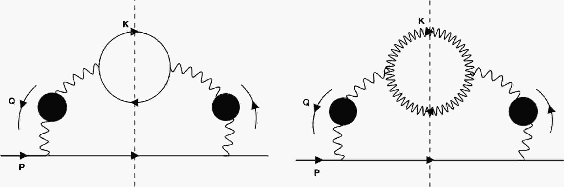
Binding energy also plays a crucial role in the inelastic scattering process, which includes Coulomb scattering and Compton scattering. It is well known that the perturbative damping rate for heavy quarks suffers from infrared (IR) divergence when the exchanged gluon carries very soft momenta [46, 47]. Fortunately, the finite binding energy, denoted as $ {{\epsilon}}_b $, sets a threshold for the energy of an exchanged gluon to dissolve the quarkonium; thus, the binding energy effectively cuts off the IR divergence, leading to a logarithmic enhancement in the binding energy. Similar IR divergence does not occur in Compton scattering as the exchanged particle is the heavy constituent [46]. At a sufficiently low binding energy, the Coulomb scattering process is logarithmically enhanced, providing the dominant contribution to the cross section. Such an enhancement of form $\ln\dfrac{T}{{{\epsilon}}_b}$ was found in [43], with T being the temperature of the QGP. Focusing on the logarithmically enhanced contribution allows one to consider only Coulomb scattering.

With Coulomb scattering, the evaluation of the dissociation rate can be reduced to the effective one-loop self-energy diagram for heavy quarks shown in Fig. 1. The gluon propagator running in the loop is the hard thermal loop (HTL) resummed propagator, which screens the IR divergence of Coulomb scattering. The remaining logarithmic divergence is cut off by $ {{\epsilon}}_b $, as we have already discussed.

Figure 1.  Self-energy diagrams for heavy quarks. The cut propagators can be put on-shell. The left/right diagram corresponds to Coulomb scattering off light quarks/gluons. The logarithmic enhancement results from the exchange of gluons with soft momenta; therefore, we must use HTL resummed propagators for them, indicated by blobs.

The question we now ask is how the vorticity enters the diagram above. We still assume the quarkonium to be unthermalized such that the vorticity affects only the light quarks and gluons. The modifications are known from quantum kinetic theories; see [48] for a recent review. Crucially, the vorticity modifies only the on-shell light quarks and gluons but not their off-shell counterparts. Aiming at vortical correction to the dissociation rate to leading logarithmic order $\ln\dfrac{T}{{{\epsilon}}_b}$, we will also restrict ourselves to the Coulomb scattering process. The role played by the vorticity is to affect the distribution and polarization of light degrees of freedom in the initial and final states.

With the light degrees of freedom polarized by vorticity, we expect a spin-dependent damping rate of heavy quarks inside the quarkonium though collisions with polarized light degrees of freedom. The spin-dependent damping rate for the constituent can further lead to a spin-dependent dissociation rate for the bound state. The spin averaged damping rate can be related to self-energy as [49]

To derive the damping rate for a particular spin state, we must project the self-energy into a spin state. To determine the appropriate spin projection operator, we first recall the following representation of the free retarded propagator for the particle state:

where $ u_s(P) $ is the eigenspinor solution to the free Dirac equation, normalized as $ u^ \dagger_r u_s=2E_p{{\delta}}_{rs} $. This is the general eigenstate representation of the retarded function in quantum mechanics applied to Dirac theory with labels of eigenstates being spin. We readily identify $ \dfrac{u_s(P){u}^ \dagger_s(P)}{2E_p} $ as the projection operator onto a specific spin state and $ \dfrac{\sum_s u_s(P){u}^ \dagger_s(P)}{2E_p} $ as the identity operator in Dirac space. With the same logic, we can rewrite the spin average in (1) more explicitly as

This suggests the following damping rate for specific spin states:

Let us comment on the validity of this representation: (4) implicitly assumes $ E_p $ to be degenerate and free eigenspinors can be used. In principle, both emanate from the solution to the following Dirac equation in the presence of self-energy:

with $ {{\Sigma}}_R $ being the retarded self-energy. However, in the perturbation theory, $ {{\Sigma}}_R\sim {{\Sigma}}^> $ is small and has a leading order contribution to $ {{\Gamma}}_s $; hence, we may ignore modifications to the energy and eigenspinor in (4), which are higher order effects.

The case of anti-particles can be analyzed similarly. Because the vorticity effect in a charge neutral QGP is expected to be identical for a particle and an anti-particle, we will focus on the damping rate for particles in the following.

Now, we are ready to calculate the self-energy of heavy quarks in a vortical QGP. As argued in the previous subsection, only Coulomb scattering contributes to the leading logarithmic order in $ {{\epsilon}}_b $, corresponding to the self-energy diagrams in Fig. 1.

The vorticity corrections to the diagrams enter through modifications of propagators for light quarks and gluons. The explicit forms are known from quantum kinetic theories. The gluon lesser propagator in the Coulomb gauge is given by [50−52]

where X is a coarse-grained coordinate labeling fluid elements. We assume a uniform temperature and slow-varying fluid velocity $ u_{{\mu}}(X) $. The vorticity is defined as $ {{\omega}}^{{\mu}}=\dfrac{1}{2}{{\epsilon}}^{{{\mu}}{{\nu}}{{\rho}}{{\sigma}}}u_{{\nu}} {\partial}_{{\rho}} u_{{\sigma}} $. $ P^{{{\mu}}{{\rho}}}_T=-{\eta}^{{{\mu}}{{\rho}}}+\dfrac{Q^{{\mu}} u^{{\rho}}+Q^{{\rho}} u^{{\mu}}}{Q\cdot u}-\dfrac{Q^{{\mu}} Q^{{\rho}}}{(Q\cdot u)^2} $ and $ P_{{{\mu}}{{\nu}}}=u_{{\mu}} u_{{\nu}}-{\eta}_{{{\mu}}{{\nu}}} $are the transverse and spatial projectors, respectively. $ {{\epsilon}} $is the sign function, and f is the Bose-Einstein distribution function. Superscripts $ (0) $ and $ (1) $ indicate the order in vorticity. $ D_{{{\mu}}{{\rho}}}^{<(1)} $ can be further simplified. In the fluid rest frame with $ u^{{\mu}}=(1,0,0,0) $, only spatial components of $ D_{{{\mu}}{{\rho}}}^{<(1)} $ are nonvanishing and are expressed as

where $ f'\equiv\dfrac{ {\partial}}{ {\partial} q_0}f(q_0) $. We have used $ {\partial}_ju_k={{\epsilon}}^{jkl}{{\omega}}_l $ in a vortical fluid and the Schouten identity $ -q_i{{\epsilon}}^{jkl}+q_j{{\epsilon}}^{kli} - q_k{{\epsilon}}^{lij}+q_l{{\epsilon}}^{ijk}=0 $ in the second equality. The greater propagator $ D_{{{\mu}}{{\rho}}}^> $ can be obtained by replacement $ f\to 1+f $ in (6). Note that $ D_{{{\mu}}{{\rho}}}^{<(1)}=D_{{{\mu}}{{\rho}}}^{>(1)} $, indicating that the spectral function is not modified at this order. The color structure is the trivial one inherited from the free gluon propagator, which we have suppressed for notational simplicity.

The quark lesser propagator is given by [53, 54]

with $ \tilde{\Omega}^{\mu\nu}=\omega^\mu u^\nu-\omega^\nu u^\mu $. $ \widetilde{f} $ is the Fermi-Dirac distribution function. Greater propagator $ S^> $ can be obtained from (8) by replacement $ -\widetilde{f}\to1-\widetilde{f} $. Again, we have $ S^{<(1)}=S^{>(1)} $, indicating no modification of spectral function at this order. In the following, we confine to the rest frame of the fluid with $ u^{{\mu}}=(1,0,0,0) $ and suppress the explicit dependence on X.

The self-diagrams adopt the same representation below:

with $ C_F=\dfrac{N_c^2-1}{2N_c} $ resulting from the color sum $ t_{ij}^at^a_{jk}=C_F{{\delta}}_{ik} $. Here, $ S_H^>(P+Q)=2{{\pi}}({\not P}+{\not Q}+m){{\delta}}((P +Q)^2- m^2) $ is the greater propagator for probe heavy quarks. $ D_{\nu\mu}^{<(1)}(Q)=-D_{\nu\alpha}^{R}(Q)\Pi^{\alpha\beta<(1)}(Q)D_{\beta\mu}^{A}(Q) $ is the vortical correction to the gluon propagator, with the correction located entirely in gluon self-energy $ {{\Pi}}_{{{\alpha}}{{\beta}}}^{<(1)} $ [55]. The gluon self-energy emanates from either the quark loop or gluon loop captured by the two diagrams in Fig. 1. $ D_{{{\mu}}{{\nu}}}^{R/A} $ represents retarded/advanced gluon propagators in the absence of vorticity, given by

$ P^T_{{{\mu}}{{\nu}}} $ is the transverse projector defined earlier, and $ u^{{\mu}} u^{{\nu}} $ is the longitudinal projector in the Coulomb gauge. We use HTL resummed propagators relevant for exchanged gluons with soft momenta [49], for which

$ m_g $ is the gluon thermal mass defined by $ m_g^2=\dfrac{1}{6}g^2T^2 (C_A+\dfrac{1}{2}N_f) $. $ x=\dfrac{q_0}{q} $, where $ q_0 $and q are the temporal and spatial components of the momentum in the QGP frame, respectively. Using (8), we obtain $ {{\Pi}}^{{{\alpha}}{{\beta}}<(1)} $ from the quark loop as

with $ T_F=\dfrac{1}{2} $ resulting from the color sum $ \text{tr}[t^at^b]=T_F{{\delta}}^{ab} $, and $ N_f $is the number of light quark flavors. Prefactor $ 2 $ occurs because vortical correction can enter either quark propagator in the loop. Clearly, $ {{\Pi}}^{{{\alpha}}{{\beta}}<(1)} $ denotes anti-symmetric indices. Using (6), we obtain $ {{\Pi}}^{{{\alpha}}{{\beta}}<(1)} $ from the gluon loop as

where $ C_A=N_c $ results from the color sum $ f^{acd}f^{bcd}=C_A{{\delta}}^{ab} $. The two terms in the square bracket in the first line correspond to vortical corrections to two gluon propagators. A symmetry factor of $ 1/2 $ is included. We now show that it is also anti-symmetric in indices. By relabeling indices $ {{\mu}}\leftrightarrow{{\sigma}} $, $ {{\nu}}\leftrightarrow{{\rho}} $ and redefinition of momentum $ K\to -K-Q $, which amounts to the interchange of two vertices, we find

Using properties $ D_{\mu\rho}^{<(0)}(P)=D_{\mu\rho}^{>(0)}(-P) $, and $ D_{{{\sigma}}{{\nu}}}^{>(1)}(P)= -D_{{{\sigma}}{{\nu}}}^{<(1)}(-P) $, we immediately find $ {{\Pi}}^{{{\alpha}}{{\beta}}<(1)}_g=-{{\Pi}}^{{{\beta}}{{\alpha}}<(1)}_g $. Moreover, $ {{\Pi}}^{{{\alpha}}{{\beta}}<(1)} $ is purely imaginary from the explicit representations (13), (14), and (6). It follows that $ D_{{{\nu}}{{\mu}}}^{<(1)} $ is also anti-symmetric and purely imaginary. The anti-symmetric property of $ D_{{{\nu}}{{\mu}}}^{<(1)} $ enables the following replacement in the product of gamma matrices in (10)

with ${{\Sigma}}^{{{\mu}}{{\nu}}}=\dfrac{\rm i}{2}[{{\gamma}}^{{\mu}},{{\gamma}}^{{\nu}}]$.

To evaluate the trace in (4), we require the following representation of eigenspinors:

$ {{\xi}}_s(s=+/-) $ are the spin up/down spinors along a given quantization axis $ \widehat{\boldsymbol{n}} $, with the following explicit expressions:

We analyze the case $ s=+ $ below. The other case can be simply obtained by flipping the direction of ${n}$. Product $ u_s(P)\bar{u}_s(P) $ is determined as

where we have defined $ \tilde{p}=\dfrac{\vec{p}}{p_0+m} $. Using replacement (17), we evaluate the trace as

Using $ D_{\nu\mu}^{<(1)}(Q)=-D_{\nu\alpha}^{R}(Q)\Pi^{\alpha\beta<(1)}(Q)D_{\beta\mu}^{A}(Q) $, the anti-symmetric property of $ {{\Pi}}^{{{\alpha}}{{\beta}}<(1)} $ and explicit representation of $ D^{R/A} $ (11), we observe that only the following contractions of gluon self-energy are required: $ P_T^{m'm}{{\Pi}}^{0m<(1)} $ and $ P^{m'm}_TP^{n'n}_T{{\Pi}}^{mn<(1)} $. These are derived in Appendix A, with the following results:

Subscripts "q" and "g" denote contributions from the quark and gluon loops, respectively. The common part of the phase space integration is calculated as

where $\int {\rm d}\cos{{\theta}}{{\delta}}((K+Q)^2)=\dfrac{1}{2kq}$, fixing $ \cos{{\theta}}=$ $ \dfrac{q_0^2-q^2+2k_0q_0}{2kq} $.

Using (4), (10), and (21) and performing the angular average of q (details given in Appendix B), we obtain the following representation for $ {{\Gamma}}_s^{(1)} $

In the above, $ s=\pm\dfrac{1}{2} $ has been inserted for the cases of both spin states. Functions $ {{\Gamma}}_1 $ and $ {{\Gamma}}_2 $ are scalar functions that depend on quark momentum p, energy $ p_0 $, binding energy $ {{\epsilon}}_b $, and temperature T, with explicit forms given by

Here, $ q_\parallel\equiv q\cdot\hat{p}=\dfrac{q_0^2-q^2+2p_0q_0}{2p} $ following from ${{\delta}}((P+ Q)^2-m^2)={{\delta}}(2P\cdot Q+Q^2)$ for on-shell P. The integration bounds of $ q_0 $ and q are given respectively by $ q_0\in[{{\epsilon}}_b, +\infty) $ and $ q\in[\sqrt{p^2+2p_{0}q_{0}+q_{0}^{2}}-p , \sqrt{p^2+2p_{0}q_{0}+q_{0}^{2}}+ p] $. Functions $ A_1^{q/g} $ and $ A^{q/g}_2(q^0,q) $ are related to the projected gluon self-energies in (22) as

In Fig. 2, we show $ {{\Gamma}}_{1} $ and $ {{\Gamma}}_2 $ as functions of p, $ {{\epsilon}}_b $, and T with $ {{\alpha}}_s=0.3 $, $ N_f=N_c=3 $, and m taken to be the charm quark mass. For simplicity, we take ${{\epsilon}}_b= 0.0233\,\text{GeV}$ for an average temperature of $ 210\,\text{MeV} $ corresponding to the weak binding scenario [56]. We find $ |{{\Gamma}}_2|\gg|{{\Gamma}}_1| $, indicating that the angular dependence of $ {{\Gamma}}_s^{(1)} $ is largely set by $ {{\omega}}\cdot\mathit{\boldsymbol{n}} $, with only a small correction from the dependence on quark momentum direction $ \hat{p} $. $ {{\Gamma}}_1 $ tends to zero as $ p\to 0 $, which is consistent with the expectation of no $ \hat{p} $-dependence in this limit.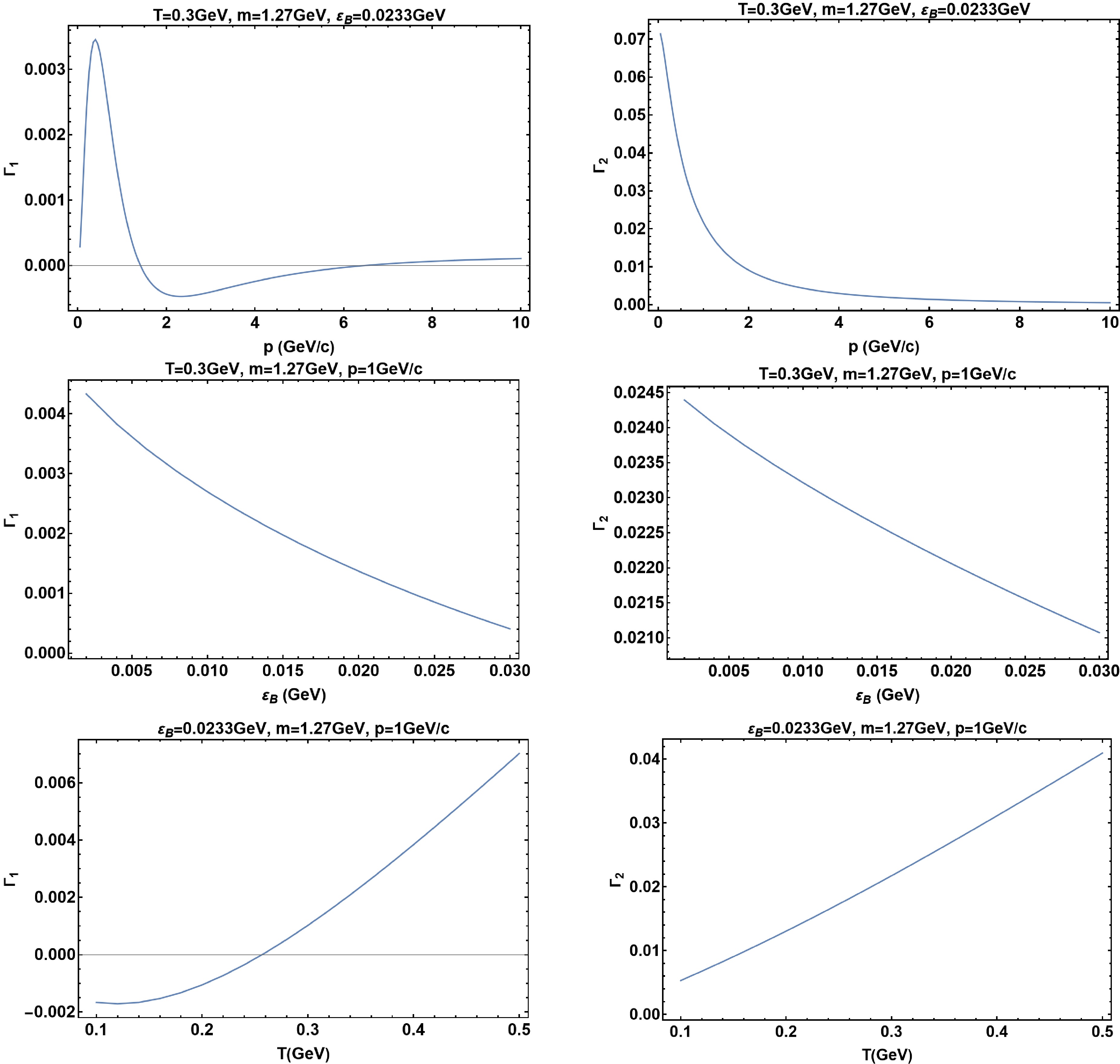

Figure 2.  (color online) $ \Gamma_1 $ and $ \Gamma_2 $ defined in (24) as functions of p, $ {{\epsilon}}_b $, and T, respectively, with $ {{\alpha}}_s=0.3 $, $ N_f=N_c=3 $, and m taken to be the charm quark mass. $ {{\epsilon}}_b $ is temperature dependent. For simplicity, we take $ {{\epsilon}}_b=0.0233\,\text{GeV} $ for an average temperature of $ 210\,\text{MeV} $ corresponding to the weak binding scenario [56]. We find $ |{{\Gamma}}_2|\gg|{{\Gamma}}_1| $ numerically, indicating that the angular dependence of $ {{\Gamma}}_s^{(1)} $ is largely set by $ {{\omega}}\cdot\mathit{\boldsymbol{n}} $, with only a small correction from the dependence on the quark momentum direction $ \hat{p} $.

A surprising result is the absence of $ \ln\dfrac{T}{{{\epsilon}}_b} $ enhancement, which we now explain. Note that $ \ln\dfrac{T}{{{\epsilon}}_b} $enhancement has indeed been found in earlier calculations of the spin-independent dissociation rate; see [43]. It results from quark coupling to fluctuations of incompletely screened chromomagnetic fields. Because two spin-magnetic vertices exist, the dependence on spin cancels in the product. In our case, the fluctuations of the chromomagnetic field can be identified with terms $ \propto|{{\Delta}}_T|^2 $ in (25) and (26). In the mean time, we have explicitly calculated the IR limit of vortical correction to gluon self-energy in Appendix C, finding the same scaling with q as their counterpart in the absence of vorticity. However, similar $ \ln\frac{T}{{{\epsilon}}_b} $ does not occur for vortical correction owing to the presence of an additional factor of $ q_0 $ in the corresponding terms. The appearance of $ q_0 $ can be understood as follows: we are seeking a spin-dependent dissociation rate. The quark can only have spin-dependent coupling to the chromomagentic field in one vertex and spin-independent coupling to the chromoelectric field in the other vertex ² such that the product is still spin dependent. The factor of $ q_0 $ is necessary for converting one of the transverse gauge fields in $ D^{m'n'<(1)}=-|{{\Delta}}_T|^2P_T^{m'm}P_T^{n'n}{{\Pi}}_{q/g}^{mn<(1)} $to a chromoelectric field. Because the chromoelectric field is completely screened, no logarithmic enhancement is observed.

Thus far, we have calculated only the dissociation from scattering with one of the constituent quarks. In the quasi-free picture, we can easily obtain the dissociation rate for quarkonia by adding contributions from two constituents:

To implement the spin-dependent dissociation rate in the spin alignment for $ {{J/{{\psi}}}} $, we take the Bjorken flow for the evolution of the QGP and the evolution of vorticity from Eq. (8) of [58]; see also [59]

For illustration, we consider quarkonia spin alignment in collisions with $ \sqrt{s_{NN}}=200\,\text{GeV} $. The temperature profile is modeled using Bjorken flow with

with $ T_0=350\,\text{MeV} $ and $ {{\tau}}_0=0.6\,\text{fm} $. $ {{\tau}}=\sqrt{t^2-z^2} $ is the proper time. Given that $ |{{\Gamma}}_1|\ll|{{\Gamma}}_2| $numerically, we ignore the term dependent on quark momentum direction $ \hat{p} $. Because the quark and anti-quark should carry close momenta in the quasi-free picture, the spin-dependent dissociation rate is nearly independent of the quarkonia momentum direction. We can then obtain a simple form of spin alignment as follows: assuming spin-independent distribution function f for initially produced quarkonia and considering the dissociation contribution only, the distribution of quarkonia in the i-th spin state is given by

with $ i=0,+,- $. Further assuming $ \mathit{\boldsymbol{n}} \parallel {{\omega}} $, we determine the corresponding spin alignment as

In the final step, we have expanded to the first non-trivial order $\int {{\Gamma}}_s{\rm d}{{\tau}}$. The $ {{\tau}} $-integration is chosen to start at $ {{\tau}}_0 $ and stop at $T=150\;\text{MeV}$. In Fig. 3, we show the p dependence of spin alignment.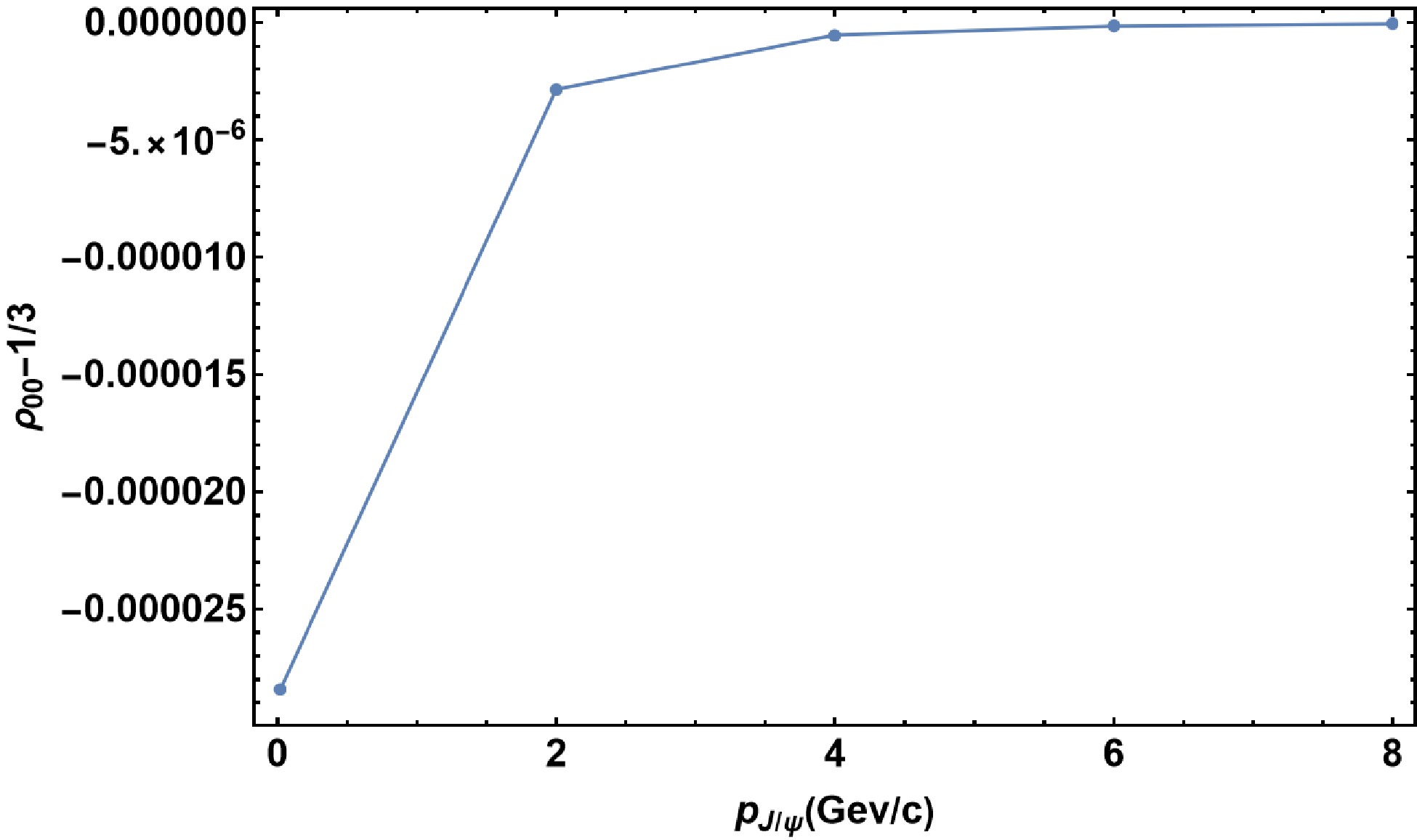

Figure 3.  (color online) Spin alignment $ \rho_{00}-1/3 $ as a function of p.

We have considered the dissociation of quarkonia in the vortical QGP and proposed the spin-dependent dissociation rate as a possible mechanism for the quarkonia spin alignment observed in heavy ion experiments. In this mechanism, small vorticity in high energy collisions may be compensated for by a long evolution time of the QGP. With QGP constituents being polarized by vorticity, inelastic scattering between quarkonium and QGP constituents naturally leads to a spin-dependent dissociation rate for quarkonia. Aiming at leading logarithmically enhanced contribution in binding energy, we focus on Coulomb scattering process in this work. We have obtained a non-trivial angular structure of the vortical correction to the dissociation rate that depends on the directions of the quantization axis, vorticity, and constituent quark momentum. The dependence on the quark momentum direction is found to be weak for phenomenologically interesting parameter choices. We have implemented the results in a simplified dissociation-dominated evolution of quarkonia, which gives a slightly suppressed spin zero states compared with the average of the other two states.

A surprising result we have found both numerically and analytically is the absence of logrithmical enhancement in the binding energy in the vortical correction to the dissociation rate. This is understood as resulting from the requirement that a spin-dependent dissociation can only come from quark coupling to a pair of chromomagnetic and chromoelectric fields. In this case, the screening effect is sufficient to render the results free of logarithmical enhancement.

Clearly, a complete study requires the inclusion of Compton scattering. Indeed, early calculations of heavy quark energy losses [46] indicate a possible significant contribution from Compton scattering, suggesting a similar contribution to the dissociation rate. A more interesting question is, how do other hydrodynamic gradients affect the spin alignment? A specific example is the shear, which can sustain for long time and is known to contribute to local spin polarization significantly [7−9]. Studying spin-dependent dissociation in a QGP with shear flow would be an interesting direction. We leave these interesting directions for future explorations.

We thank X.-z. Bai, P. Braun-Munzinger, Y. Guo, Y. Jia, M. He, D.-f. Hou, K. Zhou, P.-f. Zhuang for stimulating discussions.

We start with the evaluation of the vortical correction to the gluon self-energy from the quark loop. Working in the QGP frame with $ u^{{\mu}}=(1,0,0,0) $, we can give the explicit form of (13) as

Note that the heavy quarks are on-shell in quasi-free picture $ P^2=(P+Q)^2=m_Q^2 $. The gluon energy threshold is set by binding energy $ q_0\geq {{\epsilon}}_B>0 $. We can easily show that the gluon is spacelike as long as $ Q\ll m_Q $. Using $ {{\delta}}(K^2) $, we obtain $ {{\delta}}((K+Q)^2)={{\delta}}(q_0^2-q^2+2k_0q_0-2k q\cos{{\theta}}) $, with $ {{\theta}} $ being the angle between $ \mathit{\boldsymbol{k}} $ and $ \mathit{\boldsymbol{q}} $. $ {{\delta}}((K+Q)^2) $ fixes $ \cos{{\theta}}=\dfrac{q_0^2-q^2+2k_0q_0}{2kq} $. $ |\cos{{\theta}}|\leq 1 $ gives the following kinematic constraint on k:

For both cases, we have $ {{\epsilon}}(k_0){{\epsilon}}(k_0+q_0)=1 $. To simplify the tensor structures, we note that $ {{\Pi}}^{ij<(1)} $ should be contracted with transverse projectors on both sides; therefore, we may simply take i and j to be transverse indices. Thus, index k must be longitudinal. Formally, we can express this statement by the following identity:

The first identity can be shown by expanding it and using the Schouten identity $ {{\epsilon}}^{inl}\hat{q}^m-{{\epsilon}}^{nlm}\hat{q}^i+ {{\epsilon}}^{lmi}\hat{q}^n- {{\epsilon}}^{min}\hat{q}^l=0 $. We can then obtain projected $ {{\Pi}}^{ij<(1)} $ as

We use $ \parallel $ to denote longitudinal projection. $ k^ \parallel=k\cdot\hat{q} $. In the second line, we have made the replacement $ (k+q)_l\to (k^ \parallel+q)_l $. This is because $ k^ \perp_{{\lambda}} k^ \parallel_k $ vanishes on the angular integration of $ \mathit{\boldsymbol{k}} $. Similarly, $ {{\Pi}}^{0i<(1)}_q $ is projected as

Now, we turn to vortical correction from the gluon loop. Noting that vortical correction to either gluon propagator gives an identical contribution and gluon propagators in the loop take only spatial indices, we may write

The product of vertices in the second line above can be expressed explicitly. For $ {{\alpha}}{{\beta}}=0m $, we have

where the last term is dropped upon contraction with $P_{ij}^T(K+Q)\bigg[\dfrac{{\rm i}{{\epsilon}}^{kla}k_ak_b{{\omega}}_b}{2k_0^2}+\dfrac{{\rm i}{{\epsilon}}^{kla}{{\omega}}_a}{2}\bigg]$, which is symmetric in $ ij $ and anti-symmetric in $ kl $. For $ {{\alpha}}{{\beta}}=mn $, the product is slightly complex:

The first and last terms are symmetric in $ mn $; thus, they can be dropped ³. The remaining terms can be organized as

We then contract (39) and (40) with $P_{ij}^T(K+Q)\bigg[\dfrac{{\rm i}{{\epsilon}}^{kla}k_ak_b{{\omega}}_b}{2k_0^2}+\dfrac{{\rm i}{{\epsilon}}^{kla}{{\omega}}_a}{2}\bigg]$ and project the spatial indices to the transverse plane. For $ {{\alpha}}{{\beta}}=0m $, we have

where $ {{\omega}}_a^ \perp=({{\delta}}_{ab}-\hat{q}_{a}\hat{q}_{b}){{\omega}}_b $. In arriving at the above, we have used $ {{\delta}}((K+Q)^2) $ and made replacements such as $ k_a^\perp k_b^\perp\to\dfrac{1}{2}k_ \perp^2({{\delta}}_{ab}-\hat{q}_{a}\hat{q}_{b}) $ using rotational invariance in the transverse plane. Similarly, for $ {{\alpha}}{{\beta}}=mn $, we have

Collecting all terms, we have

We start by writing out explicit expressions of (21) as

Using (27), we may further simplify the above as

To perform an angular integration of q, we decompose $ q_k=q_k^ \parallel+q_k^ \perp $ with the parallel and perpendicular components defined with respect to $ \hat{p} $. Note that $ q_ \parallel=\dfrac{q_0^2-q^2+2p_0q_0}{2p} $ is already fixed by ${{\delta}}((P+Q)^2- m^2)={{\delta}}(2P\cdot Q+Q^2)$. Thus, we only need to perform an angular integration in the perpendicular plane. Recall that $ {{\omega}}^ \parallel $ and $ {{\omega}}^ \perp $ are defined with respect to $ \hat{q} $ instead. The angular integration can be easily performed following the same logic as the angular integration of k in Appendix A, i.e., keeping only the even power of $ q_k^ \perp $ and replacing $ q_i^ \perp q_j^ \perp\to\dfrac{1}{2}q_ \perp^2{{\delta}}_{ij}^ \perp $ with $ {{\delta}}_{ij}^ \perp={{\delta}}_{ij}-\hat{p}_i\hat{p}_j $. After straightforward calculations, we obtain

with $ \cos\varphi=\hat{q}\cdot\hat{p} $.

We will require the IR limit of (36), (37), and (44). For the quark loop contribution, the dominant contribution is from the phase space with $ K\sim T\gg Q $, which leads to the following approximation:

with subscript "q" denoting the quark loop contribution. In the above, the angular part of the k-integration is calculated as

The two pole contributions of $ {{\delta}}(K^2) $ are combined using $ \widetilde{f}(k_0)+\widetilde{f}(-k_0)=-1 $. (48) scales as $ T^2{{\omega}}/q $ with the correction suppressed by $ O(q/T) $. A similar approximation for the gluon loop contribution is

with subscript "g, hard" denoting the gluon loop contribution from hard loop momenta. (50) also scales as $ T^2{{\omega}}/q $. However, it is incomplete. Because of Bose enhancement, an additional contribution comes from the phase space with $ K\sim Q $. In this case, we may expand the distribution function $ f(k_0+q_0)\simeq \dfrac{T}{k_0+q_0}-\dfrac{1}{2} $, $ f'(k_0)\simeq -\dfrac{T}{k_0^2} $ to obtain

with subscript "g, soft" denoting the gluon loop contribution from soft loop momenta. Two contributions in (51) are from the poles at $ k_0=\pm k $, with the corresponding integration lower bound set by $ \dfrac{q\mp q_0}{2} $, respectively. We will extract the leading $ T^2{{\omega}}/q $ contribution, which clearly comes from the term $ \dfrac{T}{k_0+q_0} $ in the expansion of $ f(k_0+q_0) $. The corresponding integral can be calculated analytically. While the contributions from the poles at $ k_0=\pm k $ are separately ultraviolet (UV) divergent, their sum is UV safe ⁴. Pushing the integration upper bound to $ \infty $, we obtain

The hard parts for quark (48) and gluon (50) can be calculated and combined as

We have verified that the combination of (52) and (53) accurately reproduces a direct numerical integration of the full expressions when $ q\ll T $. Moreover, the IR limit of $ D_{m'n'}^{<(1)} $ and $ D_{0m'}^{<(1)} $given by (52) and (53) scales the same as counterpart $ D_{{{\mu}}{{\nu}}}^{<(0)} $ in the absence of vorticity.