Holography and the internal structure of charmonium

Quarkonium states produced in heavy ion collisions are important sources of information about quark gluon plasma (QGP). This state of strongly interacting matter, which behaves like a perfect fluid [1−4], is not observed directly. The reconstruction of QGP is based on the analysis of the final particles that reach the detectors in a heavy ion collision. One important tool is the analysis of suppression of charmonium states, relative to proton-proton collisions, which is interpreted as a consequence of dissociation in the medium [5, 6]. This is the reason for the wide interest in understanding the behavior of quarkonium quasi-states in a thermal medium.

The dissociation of quarkonium states in a plasma has been described in the recent literature by means of holographic models for heavy vector mesons, inspired by gauge-string duality [7−16]. In particular, the holographic model of Ref. [10] involves three energy parameters, associated with the heavy quark mass, intensity of the strong interaction (string tension), and scale of energy change in the non-hadronic decay of quarkonium. This model provides good estimates for the spectra of masses and decay constants and also for the dependence of the dissociation effect on temperature, magnetic field, density, and angular momentum [10−13, 17−19].

This phenomenological holographic model consists of a vector field in a 5-d space with some background. By requiring the field to be normalizable, one finds a discrete set of solutions corresponding to the meson states. It is important to remark that mesons are bound states of a quark-antiquark pair. The normalizable field solutions represent the different states. For charmonium, the solution with the smallest mass corresponds to $ J/\psi $. The background of the model is engineered such that the spectra of masses and decay constants are provided. However, it lacks an interpretation for the relation between the 5-d phenomenological background and the quark-antiquark interaction. The masses of the heavy meson states are a result of both the heavy quark masses and quark-antiquark interaction.

The question we address in this study is as follows: what is the relation between the 5-d background and quark-antiquark interaction? In other words, what is the relation between the background geometry and internal structure of charmonium states? To answer this, we study the holographic representation of the interaction between heavy quarks, consisting of a Nambu Goto string, in the model background. We start with the vacuum case and then analyze the finite temperature situation, where the metric develops a black hole (BH) geometry. The dissociation process of charmonium is then investigated from the perspective of the quark-antiquark interaction.

The remainder of this paper is organized as follows. In Sec. II, we review the holographic model for heavy vector mesons and present a different version, with a change in the sign of a quadratic term, which is necessary to obtain a confining background. In Sec. III, we study the quark-antiquark interaction by considering a string, with fixed endpoints, in the background of the model. Then, in Sec. IV, the finite temperature case is considered, and the dissociation process is investigated. Some final remarks and conclusions are given in Sec. V.

In gauge-string duality, the massless vector field $ V_m $ in the bulk is dual to the current operator $ j^\mu = \bar \psi \gamma^\mu\psi $, which represents a meson on the boundary ($ z \to 0 $). This correspondence provides a framework for describing mesons in terms of bulk fields. Based on this duality, a holographic model for quarkonium was proposed in Ref. [10], with an action integral of the form

with $ F_{mn} = \partial_m V_n - \partial_n V_m $. The metric $ \bar{g} $ is given by

where $ x^1 $, $ x^2 $, and $ x^3 $are the spatial coordinates of the 4-d space where the meson exists, z is the holographic coordinate, and the dilaton field is

The three parameters $ \kappa, M $, and Γ are fixed in such a way to provide the best fit for the masses and decay constants of quarkonia states.

One can incorporate the dilaton ϕ into the metric through the transformation

The new metric g is

and the action (1) takes the form

With the metric and action written as in Eqs. (5) and (6), one can interpret the dilaton as being part of the geometry of the space. This interpretation does not affect the solutions for the vector fields, as actions (1) and (6) lead to the same equations of motion for the fields. However, in gauge-string duality, it is possible to represent the potential energy associated with the interaction between heavy quarks by a string connecting two fixed points on the boundary of the 5-d space and stretching into the bulk [20, 21]. The result depends on the metric of the space; thus, metrics g and $ \bar g $ lead to different potential energies. We will revise this point in Section III. If the potential energy increases linearly with the quark-antiquark distance, one has confinement. For this to happen, the product of the metric components $ g_{tt} $ and $ g_{xx} $ must have a non-vanishing minimum, as we comment in Section III and as shown in detail in Ref. [21]. This criteria is not satisfied by metrics (2) and (5). However, if one changes the sign of the quadratic term in z in metric (5), one finds confinement. For a similar discussion, in the context of the soft wall model, see Refs. [22, 23].

If one uses the new dilaton

instead of (3) in the metric (5) when defining the metric g, it is still possible to fit the masses and decay constants of charmonium states, and the corresponding quark-antiquark potential energy will increase linearly with the quark distance, showing confinement. From now on, we consider the dilaton (7).

The action (6) leads to the equations of motion

To describe a meson at rest, we choose a solution corresponding to zero spatial momentum $ V_m(t, \boldsymbol{x}, z) = v_m(\omega,z) \mathrm{e}^{-\text{i}\omega t} $ and use the condition $ V_z = 0 $. Now, the equations of motion (8) become

where the prime symbol denotes the derivative with respect to z.

Eqs. (10) and (11) have the trivial solution $ v_t = \mathrm{constant} $, and this constant must be zero to ensure normalization. The relevant equation is (9). Choosing a fixed polarization $ \epsilon $, one can write $ v_i = \epsilon_i v $, with $ \epsilon $ a unitary vector of the form $ (0,\epsilon_1, \epsilon_2, \epsilon_3, 0) $. Then, Eq. (9) reduces to

Meson states are represented by normalizable solutions of the field. The normalization condition reads

which implies a boundary condition for the field:

The masses $ m_n $ of the charmonium states are identified with the possible energy eigenvalues $ \omega_n $ of the meson at rest, obtained by solving the equation of motion (12) with the boundary condition (14).

The decay constants are obtained from the equation [10]

where the constant $ g_5 $ is determined in Appendix A.

The equation of motion (12) with the dilaton field of (7) has no analytical solution. If only the quadratic term is present, for which $ \phi = \kappa^2 z^2 $, corresponding to the soft wall model [24], the solution is analytic and the spectrum of masses is $ m_n^2 = 4 \kappa^2 (n+1) $ $ (n = 0,1,2,3,\cdots) $, providing a nice description of light mesons.

However, for heavy mesons, experimental data show that the mass of the state $ n=0 $ is considerably greater than the differences of mass $ m_{n+1} - m_n $. This is a consequence of the fact that the masses of the heavy mesons have a very large contribution from the mass of the constituent quarks. In other words, the masses of heavy mesons depend not only on the strong interaction between the quarks but also on their masses. This is one of the reasons why a dilaton with more parameters is required when dealing with heavy mesons.

Also, heavy meson decay constants should decrease with n. This feature is not captured by the soft wall model [24], where the decay constants do not depend on n. In the tangent model, the solutions to the equation of motion (12) are numeric, but the fit of the masses and decay constants of heavy mesons is more precise.

With the definition $ \psi(z)=\sqrt{R/z}\; \mathrm{e}^{-\phi(z)/2}v(z) $, the equation of motion (12) is transformed to the Schrödinger-like form

with

This form of the equation can be used to explain the dilatons (3) and (7) and why the fit of masses and decay constants is better with these dilatons. The hyperbolic tangent in (3) or (7) adds a potential well to the potential-like function V, which is responsible for rising the decay constants of the first states. The presence of a $ \pm M z $ term on the dilaton adds a constant term to the potential, which guarantees a better fit for the masses of heavy mesons. The sign of this term was chosen in such a way that the potential in the Schrödinger-like equation leads to the best description of the charmonium states.

The best fit for the masses and decay constants is found using the following values for the model parameters:

and the obtained results are shown in Table 1. More details on this procedure of finding masses and decay constants can be found in Ref. [10].

Charmonium Masses and Decay Constants
State	Experimental Masses/MeV	Masses on the tangent model/MeV	Experimental Decay Constants/MeV	Decay Constants on the tangent model/MeV
$ 1S $	$ 3096.900 \pm 0.006 $	$ 2300 $	$ 416 \pm 4 $	411
$ 2S $	$ 3686.097 \pm 0.011 $	$ 3445 $	$ 294.3 \pm 2.5 $	259
$ 3S $	$ 4040 \pm 4 $	$ 4289 $	$ 187 \pm 8 $	206
$ 4S $	$ 4415 \pm 5 $	$ 4982 $	$ 161 \pm 10 $	180

Table 1.  Comparison of charmonium masses and decay constants obtained experimentally and from the tangent model.

The experimental values for the masses in Table 1 are taken from the Particle Data Group (PDG) [25]. While the PDG does not directly show the decay constants $ f_n $, it does provide the decay width $ \Gamma_{n \to e^{+}e^{-}} $. The relationship between these quantities is given by the formula [26]

where $ \alpha = 1/137 $ is the fine structure constant; $ c_V $ is the square of the charge of the quark, which, for charmonium, is $ c_V = c_{J/\psi} = 4/9 $; $ m_n $ is the mass of the state whose radial excitation number is n; and $ \Gamma_{n \to e^{+}e^{-}} $ is the decay width found by the PDG.

Let us define the root mean square percentage error (RMSPE) as

where $ N = 8 $ is the number of experimental points (4 masses and 4 decay constants), the $ y_i $'s are the values of masses and decay constants predicted by the model, and the $ \hat{y}_i $'s are the experimental values of masses and decay constants. With this definition, we have RMSPE=12.7%.

In the context of the gauge-gravity duality, the interaction between two static color charges, or infinite mass quarks, is represented by a string connecting the quarks. The string stretches to the fifth dimension of the $ \text{AdS}_5 $ space, with a shape that minimizes its world sheet area or, equivalently, the corresponding Nambu-Goto action [20, 21]

where $ \alpha' $ is a constant with mass dimension $ -2 $. The string endpoints are located on the axis $ x^1 \equiv x $ at the positions $ x = \pm r/2 $, and r is the quark-antiquark distance, from a gauge theory perspective.

This association was proposed by Maldacena in Ref. [20] to show that the minimal area is proportional to the expectation value of the Wilson loop along a closed contour $ \mathcal{C} $, formed by the quark-antiquark pair at $ z \to 0 $. This relationship can be expressed as follows:

Meanwhile, it is known from QCD that by taking the limit $ \Delta t\to\infty $, the Wilson loop of a quark-antiquark pair can be written as $ \left\langle W\right\rangle(\mathcal{C})\left\langle\sim\right\rangle\mathrm{e}^{-\Delta tE} $, thus giving [23]

Following Ref. [21], one can define

and

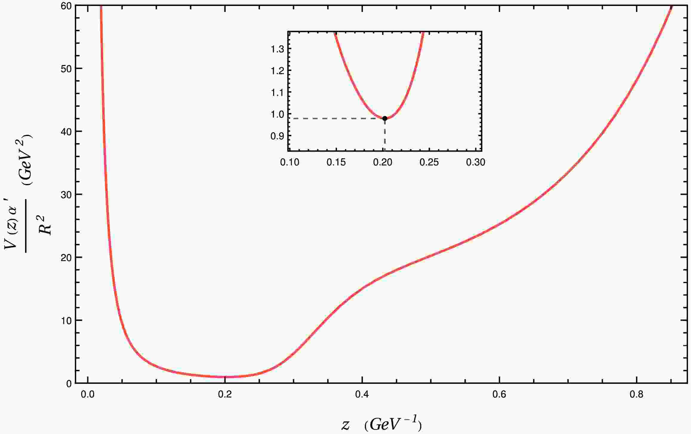
The function $ V(z) $ is plotted in Fig. 1. We designate $ z_{\min} $ as the point where the minimum of this function occurs.

Figure 1.  (color online) $ V(z) \alpha'/ R^2 $ as a function of the coordinate z.

There is no time dependence on this problem. However, one can use a Hamiltonian-based formulation, but with the coordinate x playing the role of time, to minimize the functional $ S_{NG} $. We define the Lagrangian

which leads to the Hamiltonian ¹

where

is the conjugate momentum. Note that now we are using the prime to represent derivatives with respect to the coordinate x.

As the Hamiltonian does not depend explicitly on x, its value is a constant of motion. Designating $ z_0 $ as the point where the string crosses the z axes, meaning that $ z_0 = z(x=0) $, we write

because, for a symmetric (even) and smooth string, we must have $ z'(x=0) = 0 $.

After some algebraic calculations, (29) leads to the equation of the geodesic

for the $ x < 0 $ ($ + $) and $ x > 0 $ ($ - $) sides of the string. This defines the shape of the string. Some examples of this type of string for different values of $ z_0 $ are shown in Fig. 2.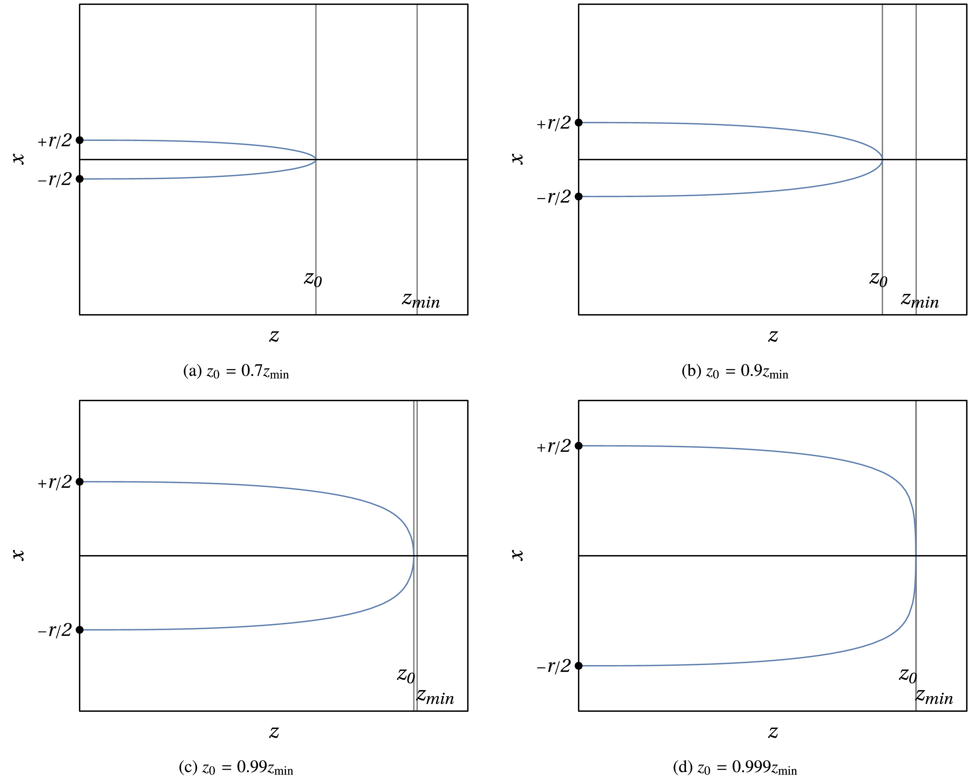

Figure 2.  (color online) Representation of four strings that are solutions of (30) with different values of $ z_0 $, corresponding to different distances r between quarks.

The string configuration is completely determined by the value of $ z_0 $ and the geodesic equation (30). In particular, the distance r between the quarks and energy E of the string can be written in terms of $ z_0 $.

At this point, note that x and z are real coordinates. Thus, $ z' = {\rm d}z/{\rm d}x $ cannot assume complex values. This implies that the argument of the square root in (30), $ V^2/V_0^2 - 1 $, must be non-negative. This condition imposes a limit on the value of $ z_0 $. From Fig. 1, note that the function $ V(z) $ is monotonically decreasing for $ z \le z_{\min} $. Thus, for strings that satisfy $ z_0 \le z_{\min} $, one has that $ V^2(z)/V_0^2 - 1 $ is always non negative. However, for $ z > z_{\min} $, Fig. 1 shows that $ V(z) $ is monotonically increasing. Thus, for a string satisfying $ z_0 > z_{\min} $, the factor $ V^2(z)/V_0^2 - 1 $ assumes negative values that would lead to a complex square root in Eq. (30). Thus, one concludes that the condition $ z_0 \le z_{\min} $ must hold.

The distance between the quarks is

It is important to note that, as we will see in the sequence, when $ z_0 \to z_{\min} $, the quark separation diverges, $ r \to \infty $.

The energy of the configuration is the length of the string

which is just the Nambu-Goto action (21) divided by the time interval.

The expression (32) is singular as it includes the infinite masses of the quarks. One can regularize the energy following a similar approach as in Ref. [20] of subtracting the contribution associated with two straight strings:

The straight strings stretch from the boundary to the minimum of the metric factor $ V(z) $, which occurs at $ z = z_{\min} $.

Now, to compare the interaction energy of the quark-antiquark pair with the Cornell potential, we analyze the asymptotic behaviors of the energy for large and small quark separation.

The asymptotic behavior of r and E for $ z_0 $ close to $ z_{\min} $ was discussed for general metrics in Ref. [21]. For the particular case of the present model, one has

and

From Eq. (34), note that the region of $ z_0 $ close to $ z_{\min} $corresponds to the region of large r. Dividing (35) by (34), we see that, in this limit,

This linear potential characterizes confinement. If it happens that, for a certain geometry, $ V(z_{\min}) = 0 $, the quarks of the dual gauge theory would be unconfined [21].

The Cornell potential [27], which effectively represents the quark-antiquark interaction for the static case, has the form

with a similar linear term in r in the large distance limit. Comparing Eqs. (36) and (37), one finds that the string tension for the present holographic model is

Meanwhile, for $ z_0 $ close to $ 0 $, one finds [28]

and

From Eq. (39), we see that the region of $ z_0 $ close to $ 0 $ corresponds to the region of small r. Therefore, multiplying (40) by (39), we see that in this limit,

Again, this is in agreement, for the small r limit, with the Cornell potential (37). The predicted coupling constant $ \alpha_s $ is

The parameters of the Cornell potential were estimated considering a charmonium state as a static system of heavy quarks and solving the non-relativistic Schrödinger equation,

for this two-body system (e.g., see Refs. [29, 30]). The eigenvalues $ E_n $ of the energy correspond to the binding energies of the system. The masses of the various charmonium states have the form $ m_n = 2 m_c + E_n $, where $ m_c $ is the mass of the charm quark. Using this approach, one is able to fix the parameters $ \alpha_s $ and σ of the Cornell potential (37) by fitting the experimental masses of charmonium states.

Following a similar approach but using our holographic potential parametrized by Eqs. (31) and (32) instead of the Cornell potential, we were able to fit the parameter $ R^2/\alpha' $. The results obtained were $ R^2/\alpha' = $ 0.0226 and the masses shown in Table 2.

Charmonium Masses from the Schrödinger equation
State	Experimental masses /MeV	Masses obtained from the Shcrodinger equation/MeV
$ 1S $	$ 3096.900 \pm 0.006 $	$ 3168 $
$ 2S $	$ 3686.097 \pm 0.011 $	$ 3652 $
$ 3S $	$ 4040 \pm 4 $	$ 4048 $
$ 4S $	$ 4415 \pm 5 $	$ 4398 $

Table 2.  Comparison of charmonium masses and decay constants obtained experimentally and from the Schrödinger equation.

This approach for calculating the masses is not equivalent to the one used in Section II. In the ideal scenario of perfect equivalence, these masses would coincide with those shown in Table 1. One could consider fitting the parameter $ R^2/\alpha' $ using the tangent model masses from Table 1 instead of the experimental values. However, this method would propagate the errors inherent to the mass fitting within the tangent model.

Therefore, using Eqs. (38) and (42), one obtains

These are the estimates from the holographic model. The value of σ is in a reasonable agreement with those obtained by the methods that apply the Cornell potential. For example, the authors of [29−31] obtained $ \sigma = {0.18} \text{GeV}^2, {0.18}\;\text{GeV}^2 $, and $ {0.164}\;\text{GeV}^2 $, respectively. Meanwhile, the value of $ \alpha_s $ is two orders of magnitude smaller than the typical values obtained from the Cornell potential. This result is consistent with the fact that the stringy description of the quark-antiquark interaction is expected to be appropriate for the large r region, while $ \alpha_s $ is related to the small r region.

Once the constant $ R^2/\alpha' $ is fixed, we use Eqs. (31) and (32) to plot the curve $ E(r) $ parametrized by $ z_0 $. This plot is shown in Fig. 3. As expected from the asymptotic calculations, this graph resembles the Cornell potential in the small and large r limits. The linear growth behavior in the large r region indicates confinement, as it implies that an infinite amount of energy would be required to separate the quarks.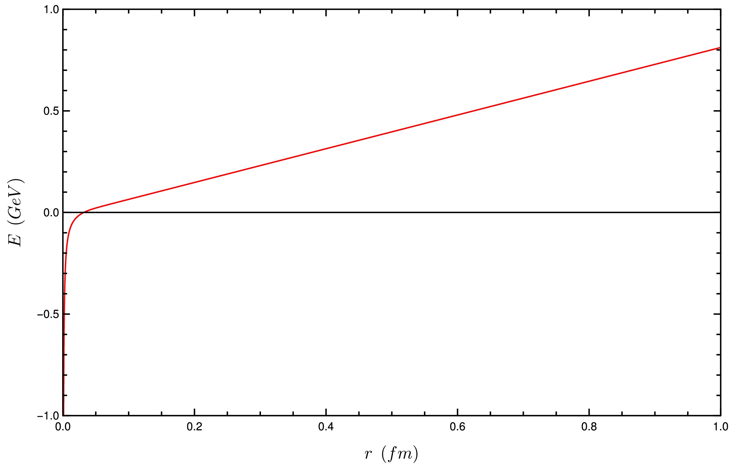

Figure 3.  (color online) Energy of the string as a function of the distance between quark and antiquark.

We introduce finite temperature by adding a black hole to our original $ \text{AdS}_5 $ space (2). The new metric is

with

The fields that represent the mesons are subject to the same action (1). Then, we introduce the dilaton into the metric, in the same way as for the zero temperature case, so that the new action assumes the same form as (6) and the new metric becomes

We assume that the dilaton parameters do not depend on the temperature. The temperature of the plasma is identified with the Hawking temperature of this black hole, which is

Inverting this equation, one can express the position of the horizon as a function of the temperature:

Using the metric (47), we generalize the definition of the function $ V(z) $ to include the dependence on the temperature:

Note that the function $ f(z) $ depends on $ z_h $ and consequently on T. Meanwhile, the function

does not change, as the factors of $ f(z) $ in $ g_{tt} $ and $ g_{zz} $ cancel out.

The variation of the function $ V(T, z) $ with the coordinate z is strongly affected by the temperature. For low temperatures, V presents two local minima: one, which is similar to the case of zero temperature, is a non-vanishing minimum at some point $ z = z_{\min}(T) $; the other is the zero of the function V at $ z = z_h(T) $. As a consequence, V also has a local maximum, located between $ z_{\min} $ and $ z_h $. As the temperature increases, this picture changes. For temperatures greater than some value $ T = T_d $, V has only one minimum, which is zero, at $ z = z_h(T) $. In this case, the local non-vanishing minimum disappears, as well as the local maximum.

In Fig. 4, plots of $ V(T, z) $ are shown for different values of temperature. In the left panel, one finds temperatures $ T < T_d $, while the right panel presents cases with $ T \geq T_d $. These plots illustrate the different behaviors. When the temperature grows, starting from a small value $ T < T_d $, the height of the local maximum decreases, and its position approaches the point $ z_{\min}(T) $. The temperature $ T_d $ is the one where both of these points, minimum and maximum, coincide, becoming an inflection point.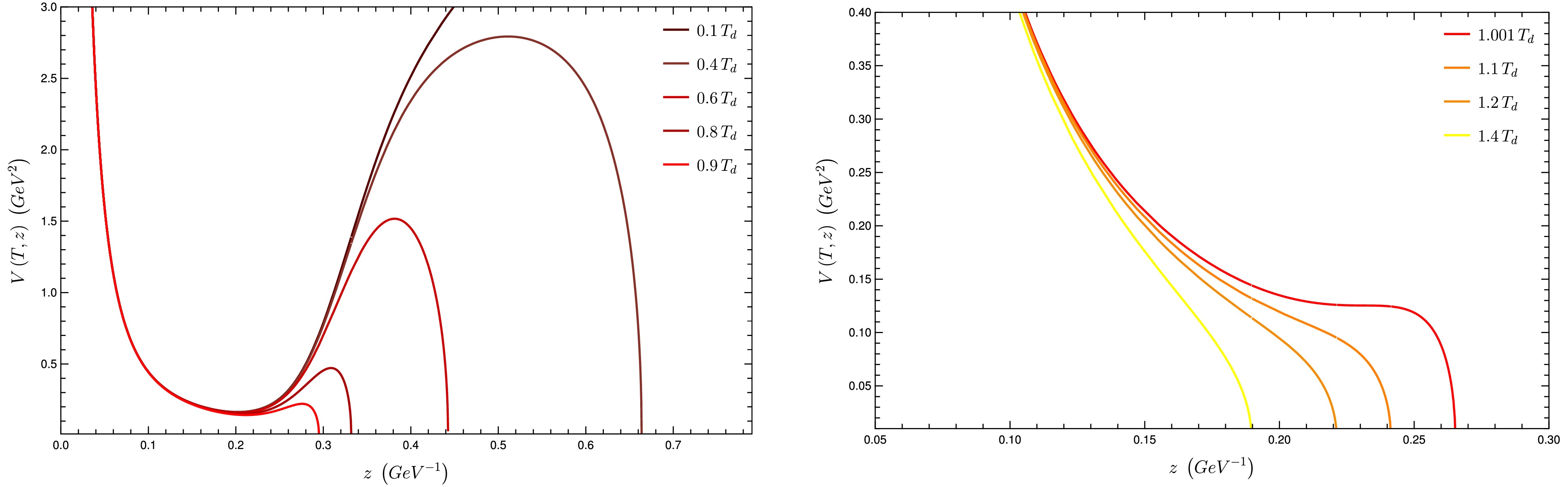

Figure 4.  (color online) Some illustrative plots of $ V(z) $ for different temperatures. In the left panel, $ T < T_d $. In the right panel, $ T > T_d $.

As we discussed in Sec. III.B, the minimum of z of the function $ V(T,z) $ is the key to determine whether there is confinement or not. For a fixed $ T \ge T_d $, the function V is monotonically decreasing with respect to z, with only one local minimum at $ z = z_h $, where $ V(z_h) = 0 $. This indicates the absence of confinement. For this reason, we call $ T_d $ the dissociation temperature. This can be determined graphically by the disappearance of the non-vanishing minimum on plots like those in Fig. 4 or by imposing that the local non-vanishing minimum and local maximum occur at the same point, which, as explained before, becomes an inflection point.

If one uses the set of parameters shown in (18), the dissociation temperature obtained from this method would be $ T_d = {1.2}\;\text{GeV} $. This value is unsatisfactorily larger than the predictions of lattice theory [32] that indicate dissociation of $ J/\psi $ at approximately $ 1.5 T_c $, where $ T_c $ is the critical temperature of the QGP formation by the dissociation of the light flavor hadrons. This corresponds to a dissociation temperature of the order of $ \, \sim {0.25}\;\text{GeV} $.

This result motivates a different procedure to fix the the model parameters: to include the dissociation temperature as one of the physical quantities to be fitted, besides the masses and decay constants. Following this approach, one finds the new set of parameters

These parameters produce the results of masses and decay constants shown in Table 3 and result in a reasonable value for the dissociation temperature.

Charmonium masses and decay constants
State	Experimental masses/MeV	Masses on the tangent model/MeV	Experimental decay constants/MeV	Decay constants on the tangent model/MeV
$ 1S $	$ 3096.900 \pm 0.006 $	$ 2399 $	$ 416 \pm 4 $	298
$ 2S $	$ 3686.097 \pm 0.011 $	$ 3560 $	$ 294.3 \pm 2.5 $	258
$ 3S $	$ 4040 \pm 4 $	$ 4011 $	$ 187 \pm 8 $	239
$ 4S $	$ 4415 \pm 5 $	$ 4590 $	$ 161 \pm 10 $	229

Table 3.  Comparison of charmonium masses and decay constants obtained experimentally and from the tangent model with parameters that give the best fit of the dissociation temperature.

The errors in the decay constants increase considerably with this new approach. The new root mean square percentage error is RMSPE = 23%, with the temperature included in the calculation.

Let us now analyze the behavior of the string and free energy in detail. The distance between the quarks has the same form as in the zero temperature case:

but now V is a function of both T and z. Because the string behavior is different depending on the temperature being lower or higher than $ T_c $, let us analyze these situations separately.

At finite temperature, one can consider an extension of the proposal of Maldacena, as discussed in Section III. Now, the Nambu-Goto action is related to Polyakov loops

As in the zero-temperature case, this expectation value is known, and in this scenario, is proportional to the free energy ²

This leads to

Note that the string that minimizes the area of the world sheet also minimizes the free energy of the system. Then, using $ \Delta t = 1/T $, we write

where the same regularization of the zero temperature case was used.

At zero temperature, we see that the domain of possible values of $ z_0 $ is $ (0, z_{\min}) $. This is necessary to prevent the quantity $ V^2/V_0^2 - 1 $ from being negative, as it is inside a square root in the geodesic equation (30). At finite temperature, for $ 0 < T < T_d $, $ z_0 $ can be in two different regions: ³ $ (0, z_{\min}) $ and $ ( \bar{z}_{\min}, z_h) $, where $ \bar{z}_{\min} $ is the point satisfying $ \bar{z}_{\min} > z_{\min} $ such that $ V(\bar{z}_{\min}) = V(z_{\min}) $. One can understand the situation by looking at the left panel of Fig. 4.

Thus, in principle, one should have to consider more than one string configuration for each temperature. However, we will see that one of them is dominant. Applying Eq. (54) to the first region, $ (0, z_{\min}) $, we find that the distance between quarks, r, increases continuously from zero, going to infinity when $ z_0 \to z_{\min} $. This behavior is similar to that found at zero temperature. Meanwhile, in the second region, r starts from a finite value at $ z_0 = \bar{z}_{\min}(T) $ and goes to zero at $ z_0 = z_h(T) $. These two behaviors can be seen in Fig. 5.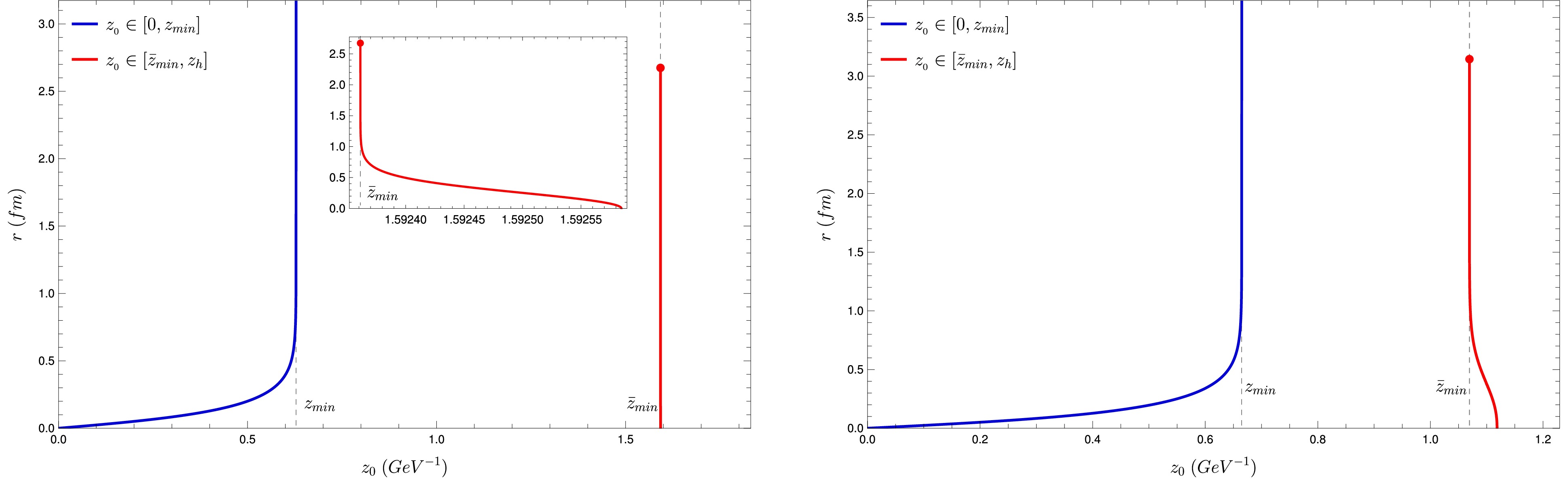

Figure 5.  (color online) Quark-antiquark distance as a function of $ z_0 $. Left panel: $ T=0.6T_d $. Right panel: $ T=0.95T_d $.

Now, using Eq. (58) for each of the two regions for a given temperature T and making the parametrization $ \left(r(T, z_0), F(T, z_0)\right) $, we find the free energy profiles plotted in Fig. 6. Note that, for $ r \in \left(0, r(\bar{z}_{\min})\right] $, there are two possibilities of energy for each r: one corresponds to a string with $ z_0 \in (0, z_{\min}) $ and the other corresponds to a string with $ z_0 \in [\bar{z}_{\min}, z_h] $. However, the string assumes the configuration that minimizes the Nambu-Goto action. Because $ F(T, z_0) $ is proportional to the action, the dominant configuration is the one that minimizes $ F(T, z_0) $ for a given r. For this reason, only the strings with $ z_0 $ in the region $ (0, z_{\min}) $ will be considered. The result for the dependence of the free energy on the quark-antiquark separation r is that of a confining potential again. The form is similar to that found in the zero temperature case, with a linear behavior for large r. A small difference that is worth pointing out is that the string tension slightly reduces when temperature grows. The result is illustrated in Fig. 7.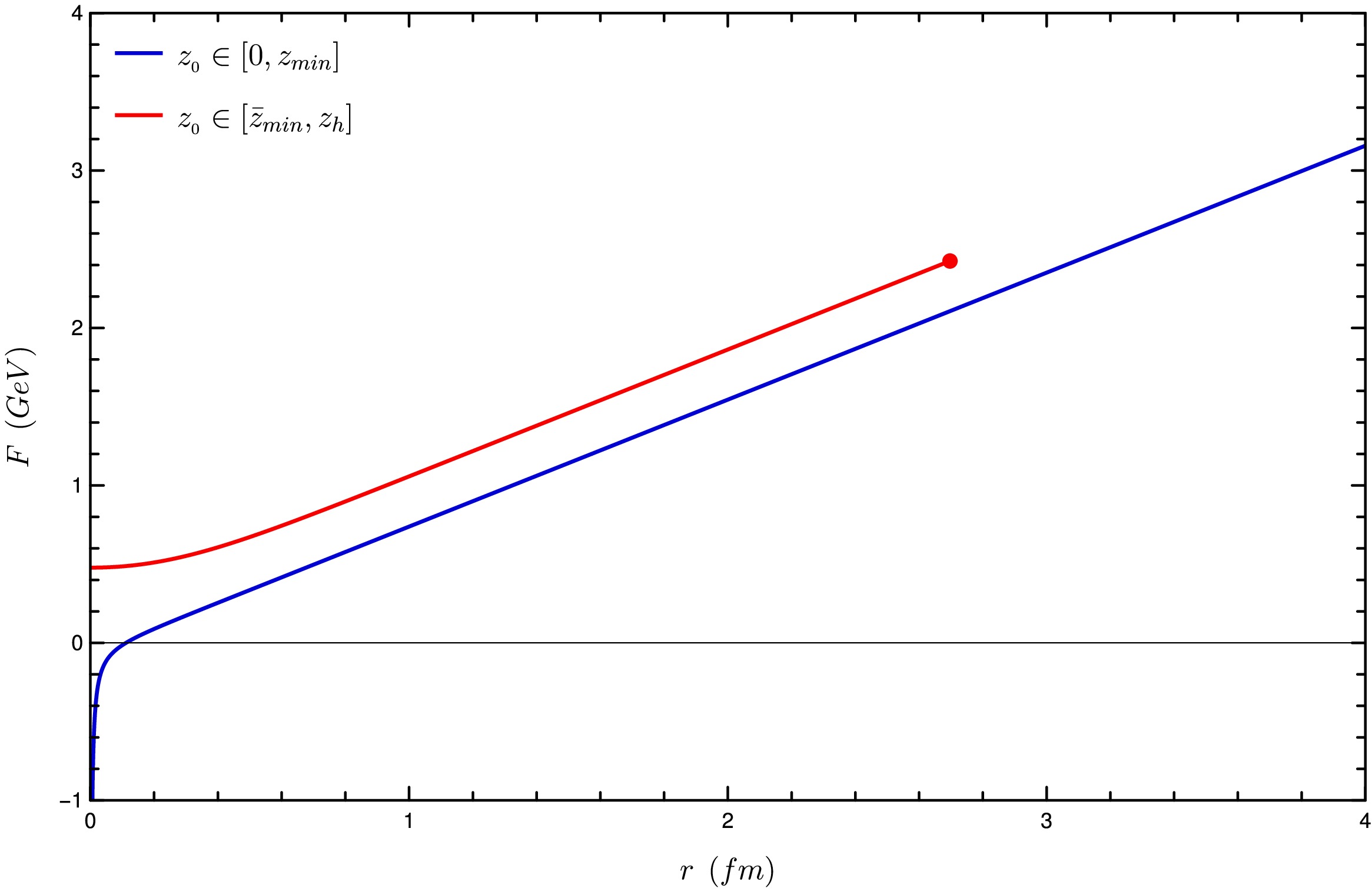

Figure 6.  (color online) Free energy F as a function of the distance between quarks r. The upper curve (red) corresponds to strings with $ z_0 $ in the region $ (0, z_{\min}(T)) $ and the lower one (blue) to strings with $ z_0 \in (\bar{z}_{\min}(T), z_h(T)] $. In both cases, $ T = 0.8 T_d $.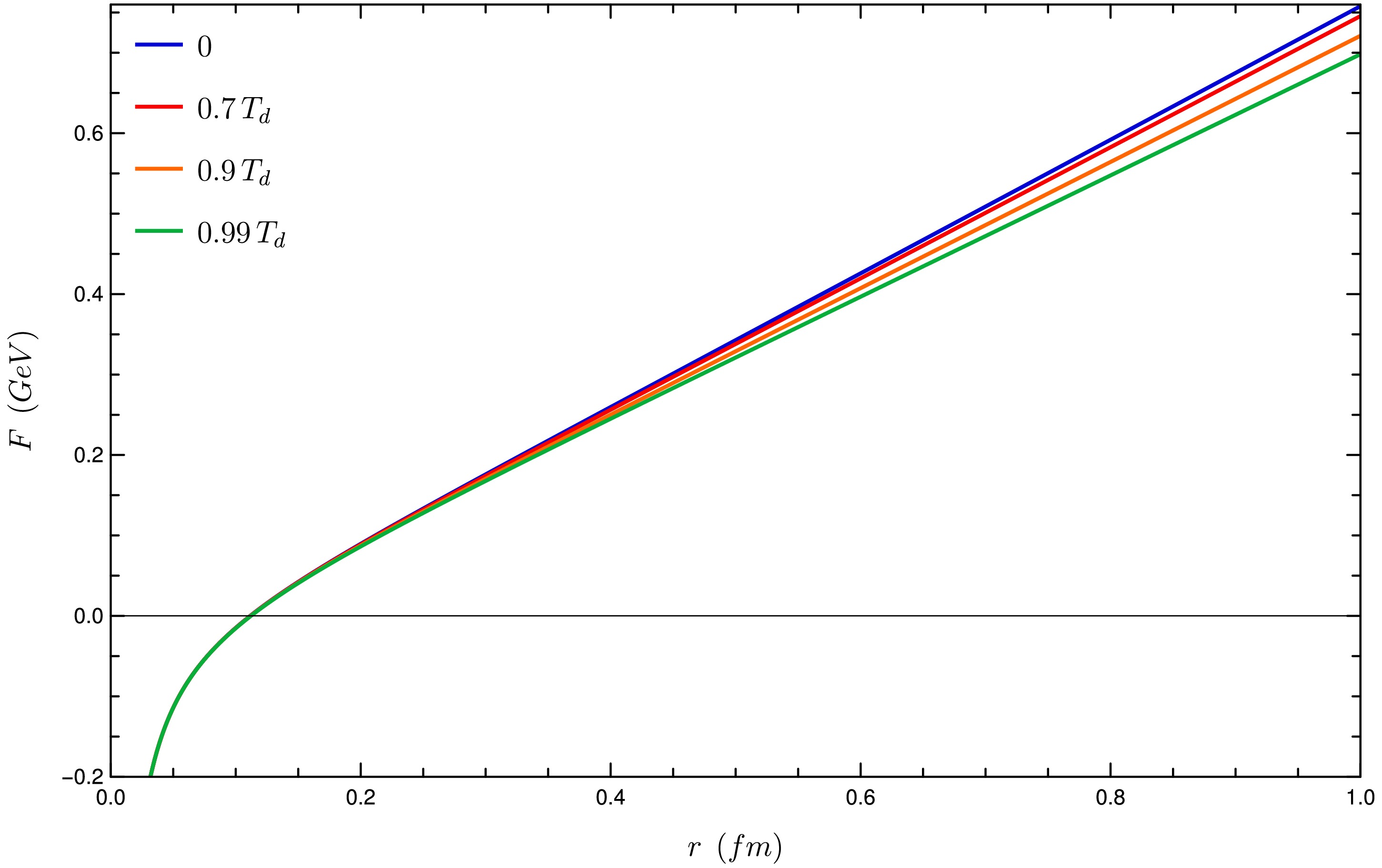

Figure 7.  (color online) Free energy F as a function of the quark separation r for four illustrative temperatures: $ T = 0; $$ T= 0.7\; T_d; \; T = 0.9\; T_d $; and$ T = 0.99\, T_d $.

For $ T > T_d $, $ z_{\min} $ does not exist anymore, so the function $ V(T, z) $ has only one minimum at $ z=z_h(T) $. In this situation, the distance between quarks, $ r(z_0) $, does not go to infinity but has a maximum value at some $ z_0 = z^* $, from which $ r(z_0) $ decreases until it reaches the value zero at $ z_0 = z_h(T) $. One can see this in Fig. 8.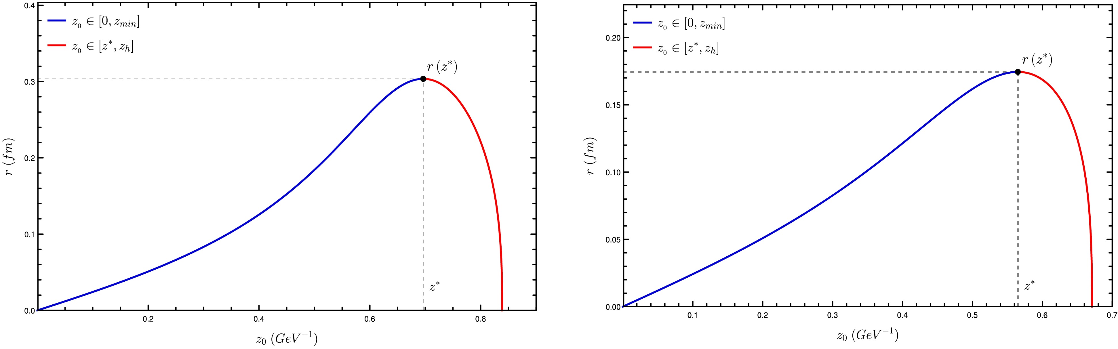

Figure 8.  (color online) Quark distance as a function of the maximum value $ z_0 $ of coordinate z. Regions: $ z_0 < z^* $ (blue) and $ z_0 > z^* $ (red). Temperatures $ T=1.2T_d $ (left panel) and $ T=1.5T_d $ (right panel).

The energy $ F(T, z_0) $ also presents a maximum finite value at $ z_0 = z^* $. For higher values of $ z_0 $, F decreases continuously until it vanishes at $ z_0 = z_h(T) $. Using the parametrization $ (r(T, z_0), F(T, z_0)) $ for some temperature $ T > T_d $, we plot the free energy as a function of the distance between the quarks in Fig. 9.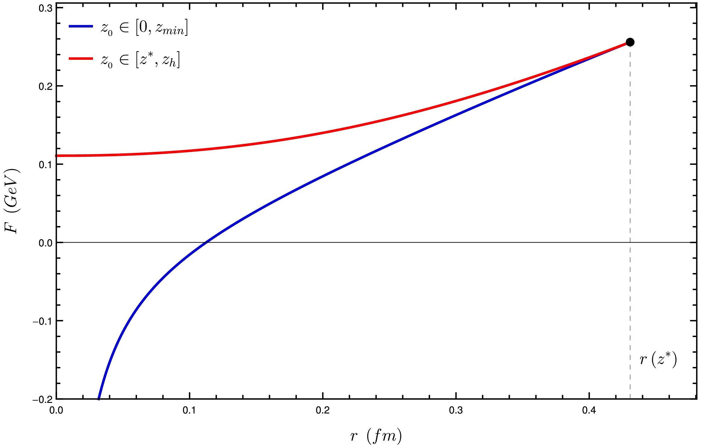

Figure 9.  (color online) Free energy as a function of quark distance at $ T = 1.01T_d $.

As one can see from Fig. 8, the region $ z_0 \in \left[ z^*, z_h \right] $ at $ T > T_d $ plays a similar role as the region $ z_0 \in \left[ \bar{z}_{\min}, z_h\right] $ did in the case of temperatures below $ T_d $. In both cases, r starts from a finite value and decreases to zero. Moreover, from Fig. 9, we see that, when comparing two strings with the same distance between quarks, the one with $ z_0 \in [z^*, z_h] $ has a value of free energy that is larger than that for the string with $ z_0 \in [z^*, z_h] $. As the string must minimize the free energy, the configuration with $ z_0 \in [z^*, z_h] $ is not formed, so we can disregard this region, similarly to what happened with the region of $ z_0 \in [z_{\min}, z_h] $ in the case with temperature below $ T_d $.

Therefore, we obtain a Cornell like potential again, but this time with a maximum range of $ r(T, z^*) $. From this point on, the quarks become free. To represent this situation, we must consider a third configuration: two lines, which represent the two quarks, going straight in the z direction up to $ z_h $, as sketched in Fig. 10. Note that these lines do not involve any variation along the x coordinate. Therefore, the corresponding energy is independent of the value of the quark separation r. This is what characterizes freedom in a two body problem: changing the distance between these bodies does not require any energy cost.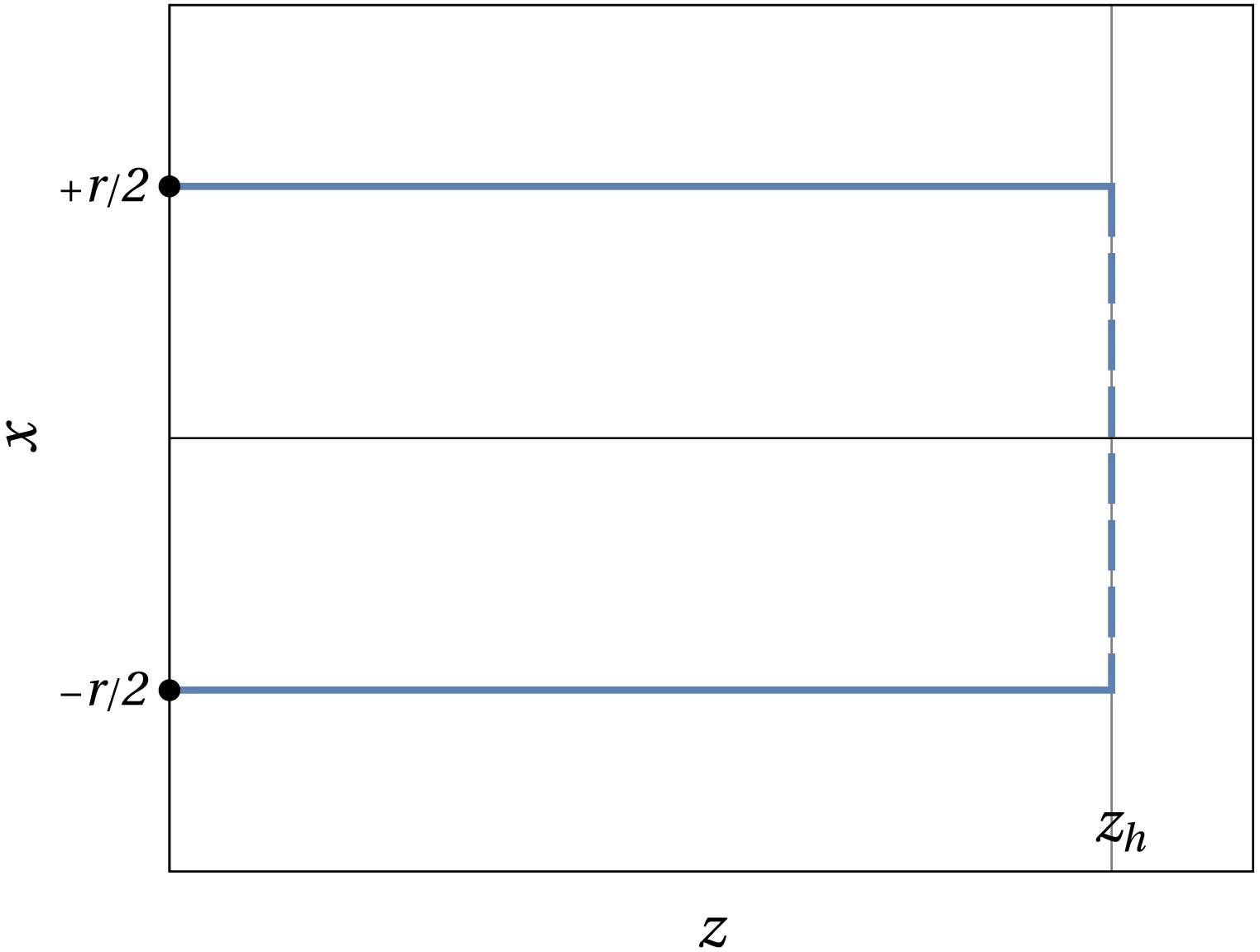

Figure 10.  (color online) String configurations corresponding to free quarks. This configuration is only formed for $ r > r_d $, and above $ T>T_d $, the energy associated with this configuration does not depend on r.

This configuration requires a different treatment to obtain the energy. Let us consider the Nambu-Goto action but now for strings that are straight lines in the z direction:

where we used the definition (51). The time interval t plays a trivial role for this static string.

Then, the energy of the set of two straight lines, which represents two free quarks, is given by

where, to avoid the singularity at $ z = 0 $, we introduced a regularization parameter $ \epsilon(T) $ that depends on the temperature. We numerically set it to a value such that the energy of the non-interacting quark pair coincides with the maximum energy $ F (r(z^*), T) $, in a manner similar to that in Ref. [33]. In other words, the parameter $ \epsilon(T) $ is chosen in such a way that the free energy is a continuous function of r.

The physical picture that emerges from this approach is non-trivial and very interesting. For temperatures larger than $ T_d $, we have an interaction given by a potential similar to Cornell's potential for small values of r. However, when the quark distance is larger than the value $ r(T, z^*) $, the energy ceases to vary with r. The corresponding string assumes the configuration of two straight lines approaching $ z_h $, with energy given by Eq. (60). The string configuration corresponding to the unconfined quarks is depicted in Fig. 10. The energy associated to this configuration $ F_\infty $ does not depend on the distance r. The resulting potential is plotted in Fig. 11 for some illustrative temperatures.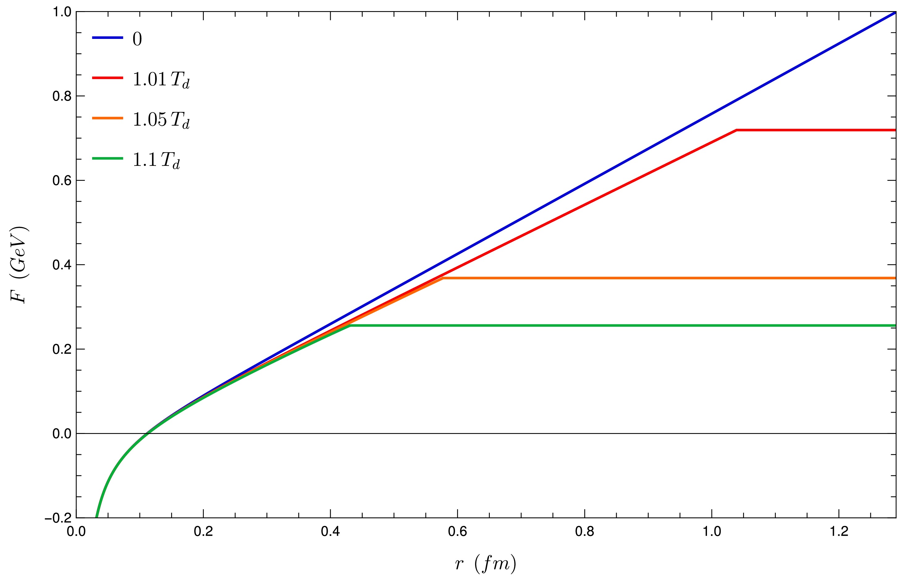

Figure 11.  (color online) Interaction energy for three temperatures larger than $ T_d $. The energy for the case $ T=0 $ is also shown for comparison.

The potential obtained is similar to the Schwinger potential predicted by QCD for quark deconfinement in the presence of temperature [34−36]. The main difference is that, in the Schwinger potential, there is a smooth transition, characterizing a crossover, whereas we observe a discontinuous transition, characterizing a first-order transition.

If we analyze large distances, it is clear that for any temperature above $ T_d $, the mesons will be deconfined, because in this limit, the string tension $ \sigma(T) = V(T, z_{\min}) = 0 $. The variation of $ \sigma(T) $ is shown in Fig. 12. Note that for this system, $ \sigma(T) $ serves as an order parameter for the confined-deconfined phase transition, being identically zero in the deconfined phase and non-zero in the confined phase. However, in contrast to lattice QCD, which indicates a continuous decrease of $ \sigma(T) $ to zero at $ T_d $ [37, 38], here, we observe a discontinuous jump to zero at $ T_d $, indicating the first-order transition.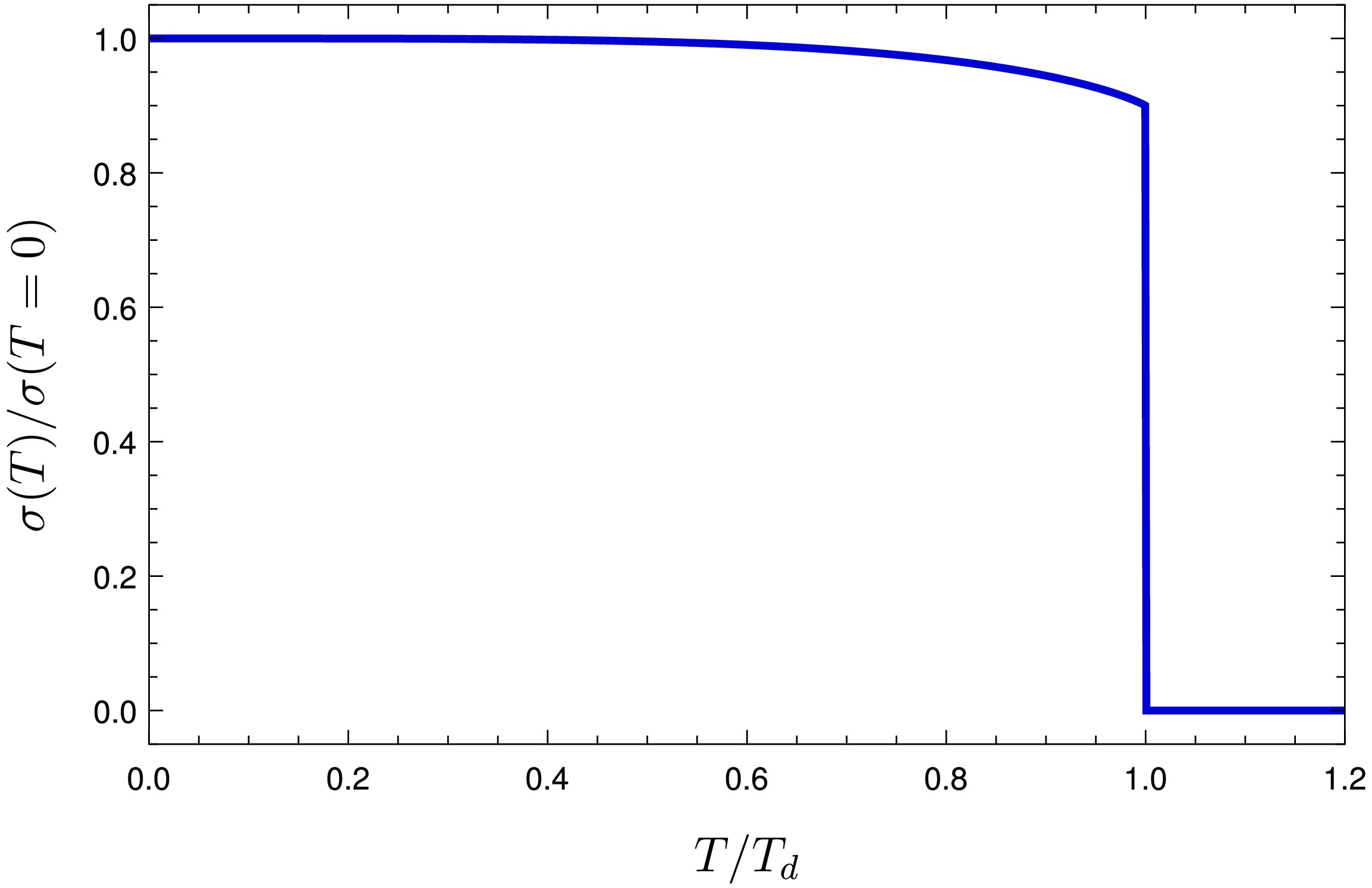

Figure 12.  (color online) String tension variation with temperature.

Looking more closely at Fig. 11, one can observe that, as the temperature increases, the maximum range of interaction decreases due to the screening effect of the medium. This maximum range is known in literature as the Debye radius $ r_d $. In Fig. 13(a), we show its dependence on temperature. Another important observation from Fig. 11 is the decrease in the free energy of the deconfined phase $ F_\infty(T) $ with temperature, as shown in detail in Fig. 13(b). These results are in qualitative agreement with the results from lattice QCD in Refs. [36−39].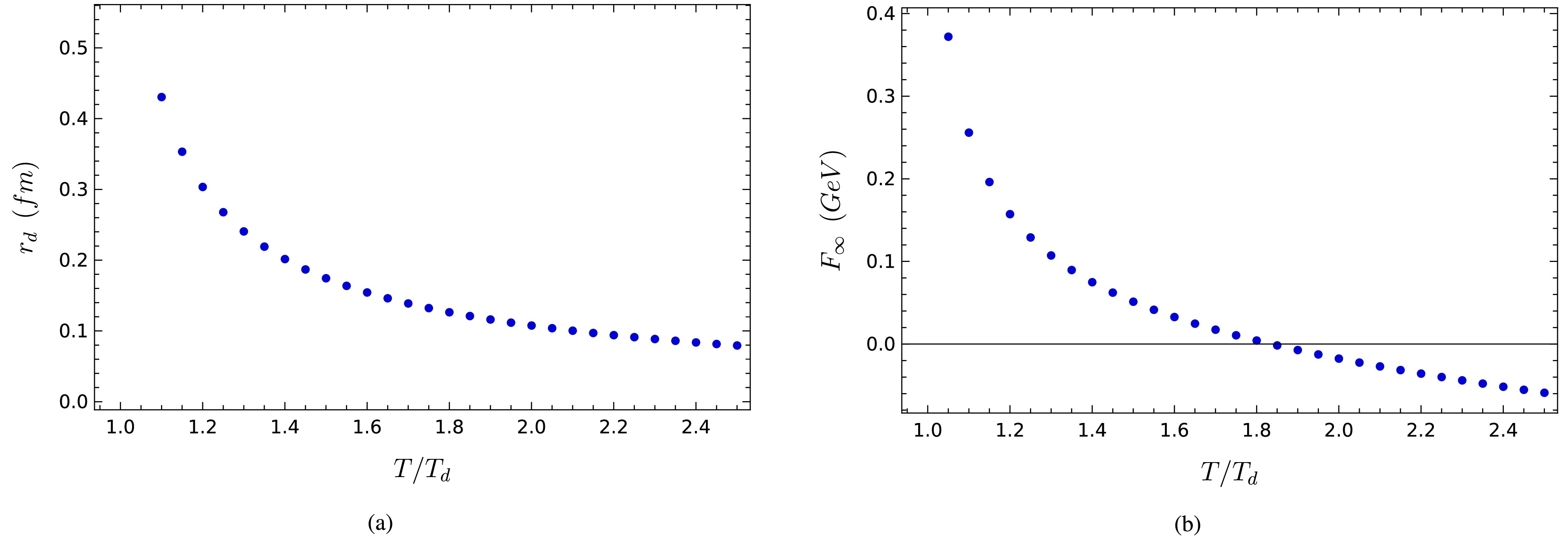

Figure 13.  (color online) (a) Maximum range of the interaction between quarks as a function of temperature. (b) Free energy of the deconfined phase as a function of temperature.

Note that, in Fig. 13(b), a region of negative energy appears for very high temperatures, corresponding to complete dissociation, where the free quarks exhibit a Coulomb-like interaction [35].

The zero temperature spectra of masses and decay constants as well as the thermal properties of quarkonium quasistates in a plasma have been successfully described recently by means of holographic models [11−16]. In these models, the heavy mesons are represented by a vector field existing in a 5-d space with some background. The main objective of the present study was to elucidate the reasons behind the ability of such a model to reproduce quarkonium properties.

In particular, we aimed to find an interpretation for the role of the extra dimension, with some non flat geometry, in the holographic models of heavy vector mesons. The guiding line of our study was the fact that mesons are not elementary particles in the strict sense but have an internal structure. A static meson can be viewed as consisting of a strongly interacting quark-antiquark pair. From a holographic perspective, the interaction of static color sources can be represented by a string existing in a 5-d background with endpoints fixed at the position of the sources. The interaction energy of the quarks is proportional to the world sheet area. For the charmonium case, we proposed adapting the procedure of Refs. [20, 21] to a background geometry corresponding to the one used in holographic models that successfully describe masses, decay constants, and the thermal behavior of quarkonium states (or quasi-states) [10−13].

It was necessary to make a change in the model of [10] because the associated background would not be confining and therefore not appropriate to describe hadrons. For a geometry to represent confinement, it is necessary that the product of the metric components in the time and transverse directions have a non-vanishing minimum. Using a set of parameters that fit masses and decay constants and also provides a confining potential for the quark-antiquark interaction, we found a potential that has the asymptotic form of the well known Cornell potential. For the limit of large quark separation, we obtained a result for the string tension compatible with the values considered in the Cornell potential in the literature.

Considering the finite temperature case, it was found that the string tension decreases with temperature up to some dissociation temperature $ T_d $. For higher temperatures $ T > T_d $, the linear term in the potential disappears for distances greater than some value that decreases with the temperature, as shown in Fig. 11. The initially obtained dissociation temperature was too high compared to lattice predictions. However, it was shown that it is possible to obtain a new set of parameters that provide a $ T_d $ compatible with expectations.

In summary, we have qualitatively shown that one can associate the 5-d background of a previous successful holographic model for charmonium as representing the internal structure of this composite particle.

To fix the constant $ g_5 $, we follow the procedure described in Ref. [40]. We start by defining the bulk-to-boundary field $ \bar{v}(\omega,z) $ as the one that satisfies the condition

where

Equation (A2) is known as the bulk-to-boundary condition.

In the region of small values of z, the equation of motion (12) in terms of the bulk-to-boundary field takes the form

The solution of this equation is

The two-point function in momentum space is calculated by

where $ \left\langle{J_\mu(x)J_\nu(0)}\right\rangle $ is given by

where the on shell action is the action (6) evaluated at the field that minimizes it. Using the fact that this field satisfies the equation of motion, it is possible to write the on shell action as

At the end, one can write the two-point function as

with

Using the bulk-to-boundary field obtained at (A.4), we find

in the limit of large $ \omega^2 $.

The constant $ g_5 $ is fixed by imposing that the propagtor obained in (A.10) matches the perturbative QCD result

where $ N_c = 3 $ is the number of color charges. This gives