MLE analysis of the relationship between the initial-state granularity and final-state flow factorization

Relativistic hydrodynamics is a widely accepted theoretical framework for modeling the temporal evolution of strongly coupled quark-gluon plasmas produced in relativistic heavy-ion collisions [1–7]. This macroscopic approach treats the plasma as a continuum, which is crucial for capturing the underlying physics that gives rise to observable phenomena. Key observables in relativistic hydrodynamics include the particle spectrum at intermediate and low transverse momenta, with particular emphasis on collective properties such as flow harmonics and correlations [8–14]. Experimentally, measurements of azimuthal distributions have been instrumental in demonstrating the concept of a perfect liquid, first observed at the RHIC [15]. Consequently, azimuthal anisotropy has emerged as a crucial observable for extracting information about the properties of the underlying physical system [16–21]. Recently, these observables have been further studied in the context of deformed nuclei [22–24].

The essence of hydrodynamical evolution can be viewed mainly as the dynamic response to fluctuating initial conditions (ICs). Given the inherently nonlinear nature of hydrodynamics, numerous studies have investigated these complex interactions. In particular, significant research has focused on understanding the relationship between initial-state eccentricities and final-state azimuthal anisotropies [25–32]. The quantitative decomposition of anisotropic ICs was first introduced in Refs. [25, 26]. This approach relies on a cumulant expansion, where each expansion coefficient captures the ''connected'' eccentricity component at a given order. Consequently, higher-order cumulants are defined by subtracting contributions from the ''disconnected'' combinations of lower-order terms. Furthermore, flow harmonics represent the hydrodynamic response to IC fluctuations, classified according to their cumulant order, with the lowest-order cumulants generally assumed to have the most significant impact.

In literature, contributions proportional to cumulants of the same azimuthal order are often identified as linear responses. In contrast, contributions from combinations of lower-order cumulants that result in the same azimuthal order are attributed to non-linearity. In practice, the response strength varies across different cumulant combinations. Specifically, the established mapping between ICs and flow harmonics is defined by the strongest correlation between an optimized linear combination of cumulant products and the corresponding flow harmonics [27, 30]. Numerical studies have confirmed that this mapping is particularly effective for more central collisions, inspiring further research in this area [28, 31, 32]. For example, one might examine whether each individual component of a given azimuthal order results in a linear response by isolating them from the IC [29]. It should be noted that each azimuthal harmonic order corresponds to an infinite set of moments or cumulants. Therefore, it remains unclear whether a specific one-to-one mapping exists or to what extent different terms of the same azimuthal order mix during dynamical evolution. Consequently, this ambiguity prompts the consideration of alternative descriptions of the radial expansion.

In this regard, some authors argued that the cumulant expansion may not be optimal for decomposing the IC. Alternatively, the Bessel-Fourier expansion proposed in Refs. [33, 34] utilizes an orthonormal basis to decompose IC fluctuations. A vital advantage of this approach is that it orders fluctuations based on their wavelength, allowing shorter wavelength radial modes to be effectively suppressed. This enables a more precise separation of different modes within a hydrodynamic framework [35]. Another intuitive method for capturing the granularity of the IC is the peripheral tube model [36–38], which provides an intuitive interpretation for the generation of triangular flow and ridge structures observed in di-hadron correlations. Unlike Fourier-based eccentricity decompositions, this model aims to capture the localized feature in the event-by-event fluctuating IC. It is motivated by heuristic arguments and numerical simulations, which suggest that high-energy-density peaks are formed near the surface region due to elementary binary collisions in the transverse plane. These localized regions naturally form a tube-like structure along the longitudinal direction and are shown to correlate strongly with the observed ridge-like structures in two-particle correlations. This model emphasizes the impact of localized IC fluctuations, as opposed to global sinusoidal expansions based on the azimuthal moment expansion. For instance, a tube located deep inside the medium, though it has a sizable contribution to the corresponding moments, would have its hydrodynamic effect significantly suppressed by the surrounding matter. In contrast, a tube near the surface can induce notable distortions in the single-particle azimuthal distribution and influence two-particle correlations. This model has been successfully employed to study various features in di-hadron correlations, showing good agreement with experimental data [36, 38–40].

The anisotropic distribution of final-state particles in momentum space is characterized by flow harmonics $ v_n $, defined through the one-particle distribution function [9, 41]

where ϕ is the azimuthal angle of the emitted particle, and $ \Psi_n $ represents the event plane for the harmonic order n. Elliptic flow ($ v_2 $) and triangular flow ($ v_3 $) are particularly relevant observables, with $ v_2 $ primarily arising from the almond-shaped geometry of the overlap region [8] and $ v_3 $ stemming from event-by-event IC fluctuations [42]. Considerable research has focused on exploring the relationship between initial geometric anisotropies and final-state flow harmonics, primarily to investigate non-linear effects [43–46], eccentricity and flow fluctuations [46–49], and multi-particle correlations [50, 51].

Various techniques have been developed to determine flow harmonics $ v_n $ from experimental data. The traditional event plane method [9, 52] estimates the event plane angles $ \Psi_n $ to evaluate the harmonics in Eq. (1), reflecting the fact that the reaction plane [42] cannot be measured directly. Other methods, such as particle correlations, use Q-vectors and cumulants [11, 53–55] to eliminate the need for $ \Psi_n $. This approach allows cumulants to be compactly expressed using generating functions [11, 56]. It includes techniques such as particle cumulants [11, 54, 56], Lee-Yang zeros [57, 58], and symmetric cumulants [59]. Recently, an alternative method based on the maximum likelihood estimator (MLE) was proposed [60], treating the flow coefficients as unknown parameters of a hypothetical probability distribution derived from experimental data. The MLE approach offers several advantages. First, it is a potential candidate to effectively handle the nonflow effects ¹, which refer to correlations that cannot be attributed to collective behavior according to Eq. (1). Momentum conservation, for example, can cause deviations from a purely flow-driven spectrum [61]. Second, the MLE is efficient at the limit of large samples and can incorporate additional constraints in the flow distribution function, making it appropriate in scenarios where a nonflow template is accessible. Furthermore, the asymptotic normality of the MLE ensures unbiased or nearly unbiased results, making it well-suited for the extensive datasets obtained at the RHIC and LHC. Given these attributes, the MLE provides a unique tool for analyzing multi-particle correlations and assessing the connection between initial anisotropy and final-state flow harmonics.

Beyond flow harmonics, the discussion can be extended to more complex observables constructed using generic multi-particle correlators. As highlighted in literature [62, 63], such quantities are often more sensitive to the specific characteristics of the underlying IC than their global averaged properties. Specifically, event-by-event fluctuations in the IC can introduce significant effects in multi-particle correlators, leading to transverse momentum ($ p_{\rm T} $) dependent event planes [48]. To capture these variations, the final-state event planes are typically estimated using the azimuthal distribution of particles over a broad $ p_{\rm T} $ range on an event-by-event basis. Experimental data [64, 65] and hydrodynamic simulations [42, 48] indicate that the event planes fluctuate significantly across different $ p_{\rm T} $ intervals. This observation, which is supported by studies such as Refs. [66–68], reveals that the correlation matrix in transverse momentum can be approximately factorized. Such factorization is considered compelling evidence for the hydrodynamic picture of heavy-ion collisions. Consequently, flow factorization [48, 62, 63] has emerged as a powerful tool for probing the properties of initial-state fluctuations.

The breakdown of flow factorization is primarily attributed to event-by-event fluctuations in the initial energy distribution [48, 62, 63, 66, 67] rather than to variations in the transport properties of the medium. This suggests that a detailed analysis of factorization breakdown can yield valuable insights into the IC of the system. Moreover, distinct differences have been observed between flow Pearson correlations constructed using different moments [69]. Given the ability of the MLE to preserve the structure of these correlations owing to its equivariance properties, it provides a robust and meaningful framework for assessing multi-particle correlators and their sensitivity to initial-state granularity.

The present study is motivated by the above considerations. We aim to explore the relationship between initial-state anisotropies and final-state flow harmonics and their correlations by employing the MLE as a statistical estimator for the flows and other higher-order moments. Specifically, we use the peripheral tube model to quantify IC granularity and employ flow factorization to capture nuances in high-order flow harmonics and multi-particle correlators. In particular, the MLE has been applied to specific correlators that are otherwise inaccessible for an arbitrary combination.

The remainder of this paper is organized as follows. In the next section, we discuss the MLE as a statistical estimator for multi-particle correlators and flow factorization. In Sec. III, we introduce the peripheral tube model and describe its application in modeling ICs with varying granularity. Numerical studies, investigating the relationship between IC granularity and final-state flow factorization, are described in Sec. IV. The results are compared with those obtained using cumulants and the event-plane method. The final section provides further discussions and concluding remarks.

The most prominent methods for extracting flow harmonics are based on multi-particle correlations [52]. These techniques rely on the following definition for a k-particle correlator [47]:

where $ \langle\cdots\rangle $ denotes the average over distinct tuples of particles, assuming independent particle emission as described by Eq. (1) in the limit of infinite multiplicity.

To isolate $ v_n $, one typically chooses a specific set of indices $ (n_1, \cdots, n_k) $ such that [47]

which ensures that all contributions from the event planes cancel in the exponential. This condition effectively reduces the expression to a formalism independent of the event-plane angles [50]. The simplest example is the two-particle correlation ($ k=2 $), where $ n_1 = -n_2 = n $. This choice yields

which directly relates the two-particle correlation to the square of the flow harmonic $ v_n $.

In realistic scenarios, however, the number of particles (M) in a given event is finite. Thus, the analysis is performed using discrete azimuthal angles $ \phi_1, \phi_2, \cdots, \phi_M $ corresponding to the measured particles. Rather than employing the integration in Eq. (4), which is not viable for a finite number of particles M, it is intuitive to use the summation [59]

to estimate the flow harmonic $ v_n $.

As a more sensitive observable, flow factorization is defined as a Pearson correlation in terms of flow vectors evaluated at different transverse momenta, namely,

where $ p_{\rm T}^{\rm t} $ and $ p_{\rm T}^{\rm a} $ are transverse momenta of the trigger and associated particles, respectively, and $ V_{n\Delta}(p_{\rm T1},p_{\rm T2}) $ is the nth harmonic of the underlying di-hadron azimuthal distribution with transverse momenta $ p_{\rm T1} $ and $ p_{\rm T2} $, namely,

where

is known as the flow vector [70, 71]. Because of its explicit consideration of transverse momentum dependence, Eq. (7) can be viewed as the differential counterpart of the two-particle correlation defined in Eq. (4). Similar to Eq (5), in practice, Eq. (7) is implemented by enumerating all possible combinations of the measured particles, as given in Appx. A of [69]

From a statistical inference perspective, Eq. (5) serves as an estimator, providing an estimation of $ v_n^2 $ rather than $ v_n $ itself, based on a finite number of observations. The first two moments of this estimator can be readily evaluated [60] and generally do not vanish. Specifically, this estimator has a finite variance that decreases with increasing multiplicity. For higher-order correlators, one can employ generating functions [11, 72, 73] or compute them directly [54] using Q-vectors [53] or flow vectors [70, 71]. Notably, quantities constructed using Q-vectors or flow vectors can also be interpreted as estimators, serving as generalized extensions of the unweighted sums in Eq. (2). Notably, the variance of these quantities largely remains finite [74], indicating an inherent statistical uncertainty due to the finite number of measured events and particle multiplicity. A finite variance implies that uncertainties in the estimated flow harmonics are inevitably influenced by limited statistics, particularly for a finite number of events. Therefore, such limitations of statistical origin must be considered when comparing results obtained from different flow measurement methods.

Following this line of reasoning, the MLE could serve as an alternative estimator for flow and related observables, a possibility explored in a previous study [60]. Expressly, for a given set of observations $ y\equiv (y_1, y_2, \cdots, y_M) $, we assume that they are sampled from a joint probability distribution governed by several unknown parameters $ \theta \equiv (\theta_1, \theta_2, \cdots, \theta_m) $. As mentioned in the Introduction, the likelihood function $ {\cal{L}} $ for the observed data is given by

which represents the joint probability density for the given observations evaluated under parameters θ. The goal of the MLE is to determine the parameters for which the observed data attain the highest joint probability, namely

where Θ is the domain of the parameters. In particular, for independent and identically distributed (i.i.d.) random variables, $ f(y; \theta) $ is given by a product of likelihood functions $ f^{\rm{uni}} $:

This scheme can be readily applied to collective flow in heavy-ion collisions. Considering an event consisting of M particles, the likelihood function reads

where the likelihood function $ {\cal{L}} $ is governed by the one-particle distribution function expressed in Eq. (1). The last equality is based on the assumption that the particles' azimuthal angles are i.i.d. variables. The parameters of the distribution, $ \theta = (v_1, v_2, \cdots, \Psi_1, \Psi_2, \cdots) $, are the flow harmonics and event planes.

In practice, one often chooses the objective function to be the log-likelihood function $ {\ell} $:

Numerical calculations indicate that Eq. (13) is more favorable than Eq. (12), although as multiplicity M increases, an appropriate implementation should be adopted to avoid increasing truncation error.

The maximum of $ \ell $ occurs at the same value of θ that maximizes $ {\cal{L}} $. For $ \ell $ that is differentiable in its domain Θ, the necessary conditions for the occurrence of a maximum are

As discussed in the Introduction, the MLE has asymptotic normality, which attains the Cramér-Rao lower bound as the sample size increases. In other words, no consistent estimator has a lower asymptotic mean squared error than the MLE. In the context of relativistic heavy-ion collisions, all events of a given multiplicity asymptotically form a (multivariate) normal distribution:

where $ \theta_0 $ represents the true value, and $ I_M(\theta) $ is the Fisher information matrix, defined as

where the expectation $ E_\theta $ is taken with respect to the distribution $ f(\phi_1,\cdots,\phi_M;\theta) $. For i.i.d. data, the Fisher information possesses the form

where $ I_1 $ is the Fisher information matrix for a single observation. As a result, the standard deviation of the MLE is expected to be roughly proportional to $ \dfrac{1}{\sqrt{M}} $. As an asymptotically normal and unbiased estimator, the MLE is mathematically guaranteed to be superior to any other estimator as the sample size becomes sufficiently high. However, for a given event, this is limited by the number of particles emitted from the collision. The overall uncertainties receive contributions from both factors. In practice, the two estimators give similar results for flow harmonics [60], with minor uncertainties of the same magnitude.

The peripheral tube model [38] offers a simplified yet effective framework for understanding the generation of triangular flow and the resulting particle correlations. This approach is intrinsically connected to event-by-event fluctuating hydrodynamics, where the ICs are represented by a few high-energy tubes near the system's surface. Each of these high-energy tubes independently influences the local hydrodynamic evolution, and these tubes' collective contributions combine to produce the observed particle correlations.

The present study utilizes the tube model to quantify the granularity of the fluctuating IC, while the bulk of the hot matter is substituted by an average energy density distribution obtained from multiple events of the same centrality class. We systematically vary the size and number of these tubes to investigate their impact on flow harmonics and particle correlations, focusing on flow factorization. The IC in this model is devised to reflect the underlying event-by-event fluctuating initial energy density distribution, consisting of two main components: a smooth background and several high-energy-density tubes close to the surface. The smooth background captures the bulk properties of the system, while the tubes represent localized fluctuations on an event-by-event basis. The energy density profile in the model is expressed as

where the average background distribution $ \epsilon_{\rm{bgd}} $ is given by

and the radial coordinate is defined as

where the constants $ K,\; L,\; M,\; a,\; b $, and c are given in Table 1. These model parameters are determined by fitting to the average ICs generated by a microscopic event generator, such as NeXuS [75, 76] or EPOS [77–79]. The energy density profile given by Eq. (19) features an almond-shaped plateau in the middle and then decreases rapidly at the edge. The specific values were extracted to match the average ICs for the mid-central 20%−40% window of 200 A GeV Au+Au collisions [80].

K	L	M	a	b	c	$ A_{\rm{tube}} $	$ R_{\rm{tube}} $
9.33	7.0	2.0	0.41	0.186	0.9	12.0	2.3

Table 1.  Parameters of the peripheral tube model employed in the present study.

The profile of an individual high-energy tube is given by

where $ A_{\rm{tube}} $ and $ R_{\rm{tube}} $ denote the maximum energy density and radius of the tube, respectively. Their specific values were also extracted [80] from a typical high-energy bumpy structure encountered in events generated by the microscopic event generator. The radial position $ r_{\rm{tube}} $ is defined as

with the spatial coordinates $ (x_{\rm{tube}}, y_{\rm{tube}}) $ given by

Here, the parameters $ r_0 $, a, b, and θ determine the radial location and orientation of the tube. Eq. (22) dictates that the distribution of the tubes primarily follows the almond shape of the background. In the present study, the number of tubes is varied to reflect the different degrees of granularity of the IC. Previous analysis suggests that this parameter has a limited effect on the resulting flow harmonics and two-particle correlations [81]. Nonetheless, as shown below, varying the granularity has a relatively subtle effect on the resulting collective flows. The parameters used in this model are calibrated using typical IC profiles for Au+Au collisions in the $ 0\%-5\% $ centrality class at $ \sqrt{s_{NN}} = 200 $ GeV. For a randomly generated event, the radii and azimuthal angles of the tubes are drawn from the uniform distributions $ r_0 \sim {\rm{U}}(0, 0.546) $ and $ \theta \sim {\rm{U}}(0, 2\pi) $, respectively. The model parameters are summarized in Table 1.

Using the devised IC furnished with the peripheral tube mode, the final-state particles are obtained by numerical simulations using the hydrodynamic code NeXSPheRIO [38, 82]. NeXSPheRIO is a hydrodynamic code using a mesh-free Lagrangian method known as smoothed particle hydrodynamics. It adopts event-by-event fluctuating ICs furnished with microscopic event generators such as NeXuS and EPOS. The temporal evolution is implemented for a three-dimensional ideal fluid. At the end of the hydrodynamic evolution of each event, a Monte-Carlo generator is employed to achieve hadron emission in Cooper-Frye and chemical freeze-out prescriptions [83]. Subsequently, hadronic decay is considered. In this study, the temporal evolution is evaluated in a 2D+1 manner, along with differential flow harmonics and multi-particle correlations, in terms of flow factorization. The calculations are performed for IC configurations with different numbers of tubes $ N_{\rm{tube}} $. The numerical results are shown in Figs. 1−4.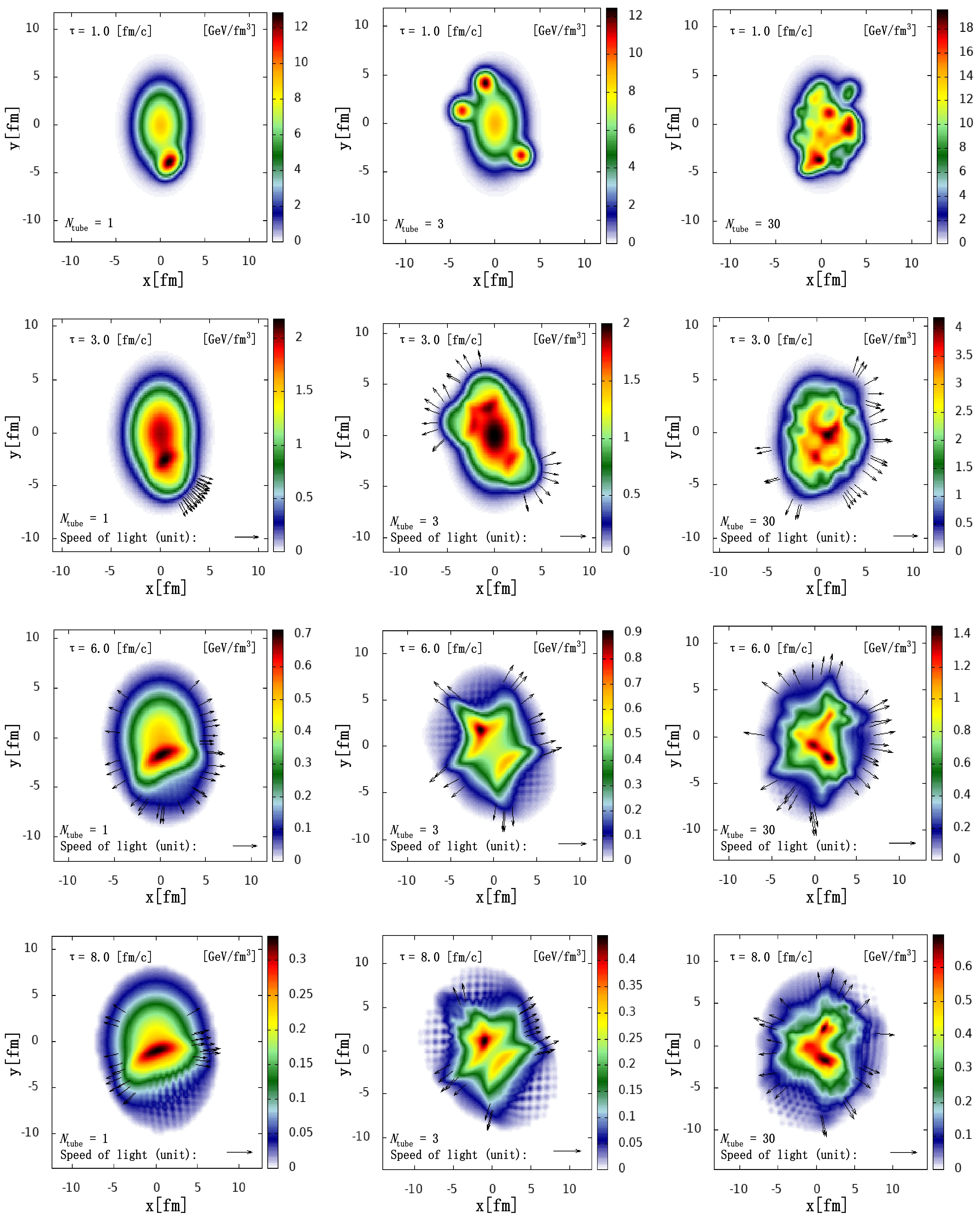

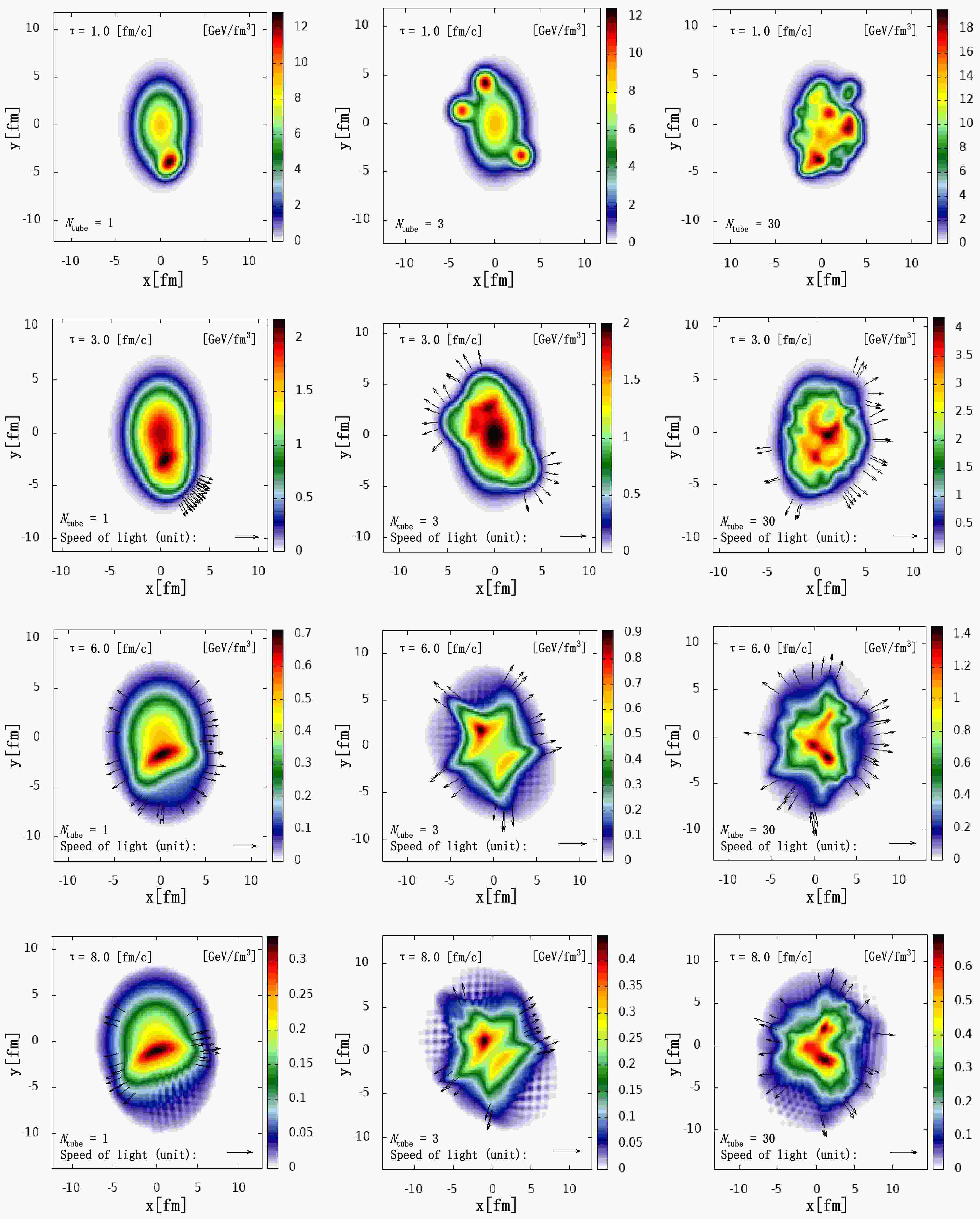
Figure 1.  (color online) Temporal evolutions of different IC configurations with $ N_{\rm{tube}} = 1 $, 3, and 30 tubes. The hydrodynamic simulations are carried out using the NeXSPheRIO code. It is observed that the hydrodynamic expansion of the system can be drastically different for different ICs.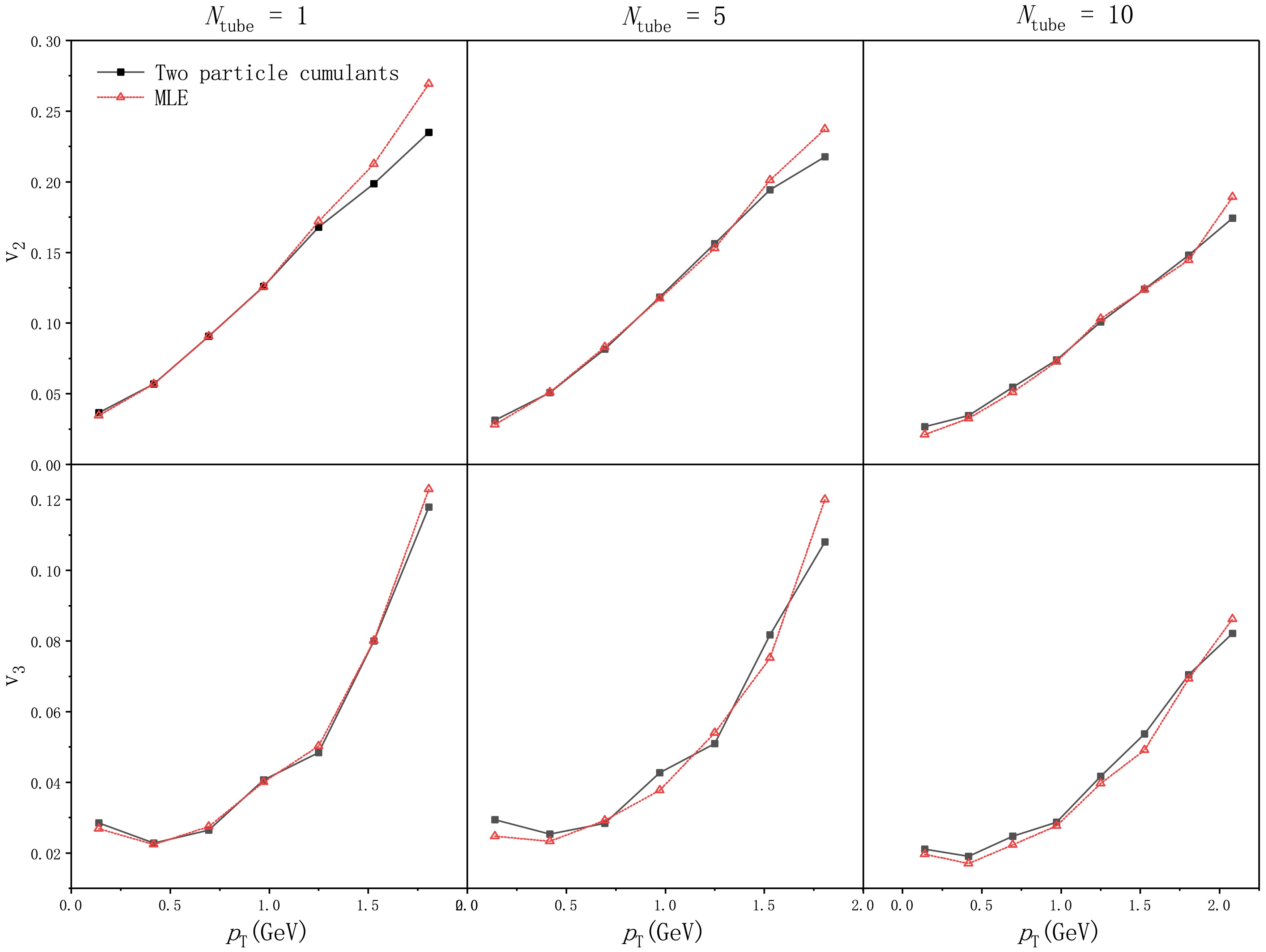

Figure 2.  (color online) Event-by-event averaged elliptic and triangular differential flows for ICs with different numbers of tubes $ N_{\rm{tube}} $. The numerical calculations are carried out using the MLE and particle cumulant methods.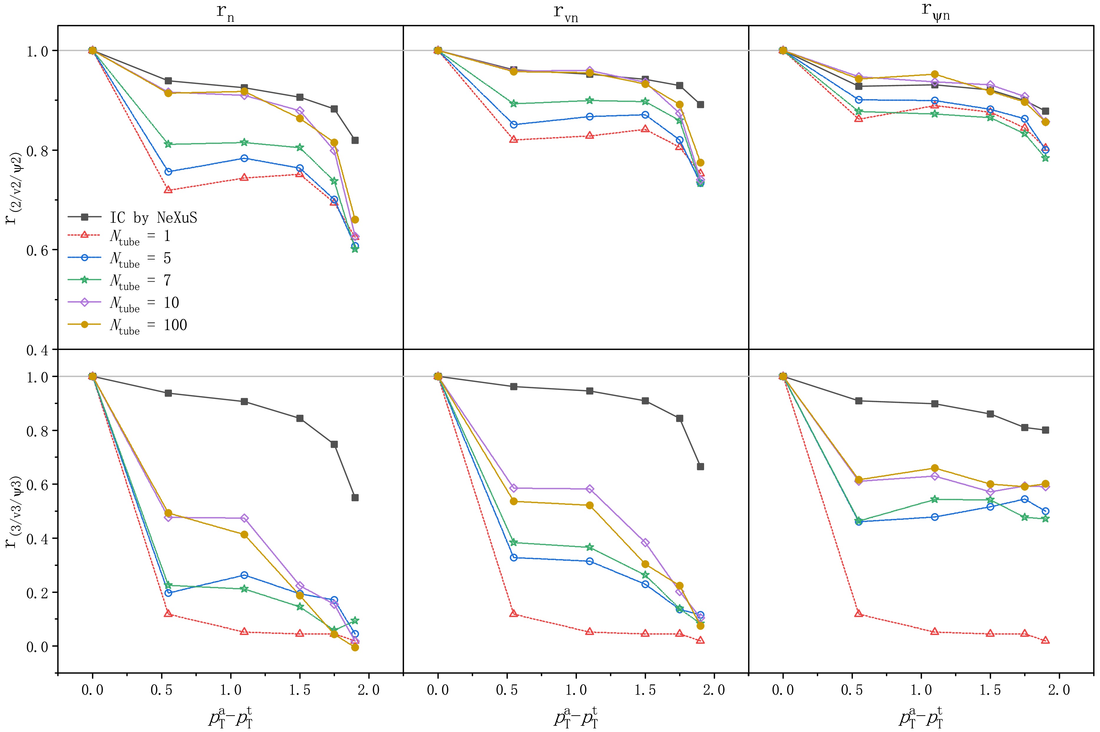

Figure 3.  (color online) Obtained flow factorization ratio $ r_n $, flow harmonics, and event-plane correlations as functions of $ p^{\rm a}_{\rm T}-p^{\rm t}_{\rm T} $ for event-by-event fluctuating ICs generated by randomly casting $ N_{\rm{tube}}=100 $peripheral tubes. The results are also compared against event-by-event fluctuating ICs generated by NeXuS, as shown by black filled squares. The numerical calculations are carried out using the MLE method. From left to right, the three columns correspond to factorization ratio, flow magnitude, and event-plane correlations. The top row shows the results for $ r_2 $, while the bottom row displays the calculated $ r_3 $.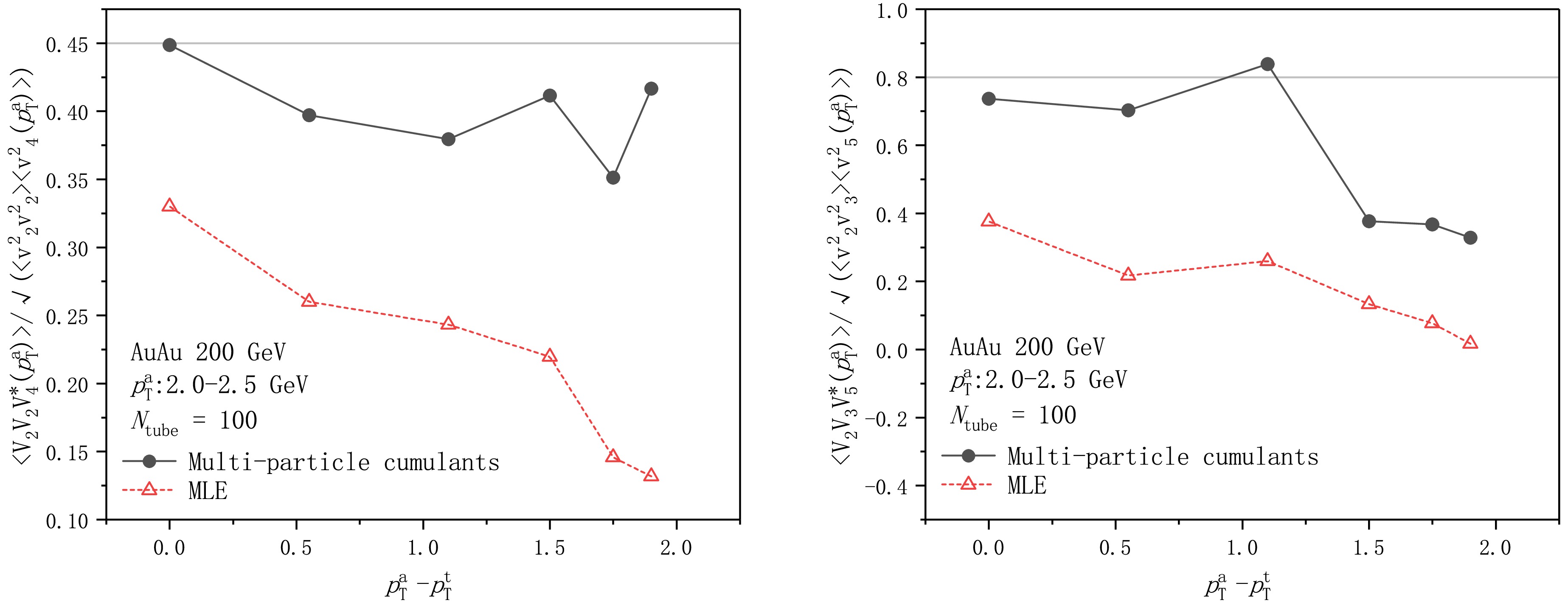

Figure 4.  (color online) Mixed harmonic factorization ratios as functions of $ p^{\rm a}_{\rm T}-p^{\rm t}_{\rm T} $ for event-by-event fluctuating ICs generated by randomly casting $ N_{\rm{tube}}=100 $ peripheral tubes. The left panel shows the ratio as a function of momentum interval for $ m=5 $, $ k=3 $, and $ n=2 $, and the right panel presents that for $ m=4 $, $ k=2 $, and $ n=2 $. The calculations are carried out using the MLE and multi-particle cumulants.

As shown in Fig. 1, the dynamic evolutions can drastically differ depending on different IC configurations. As demonstrated in the left and middle columns of Fig. 1, when there are only a few tubes, the fluid is observed to be deflected in the vicinity of each tube to both sides. In particular, the evolution around an individual high-energy tube leads to two peaks separated by approximately$ 120 $ degrees in the azimuthal distribution, as indicated by the left-most column of Fig. 1. Subsequently, this gives rise to the desired two-particle distribution where a double peak is formed on the away side, as pointed out in previous studies [ 39]. However, as the number of tubes increases, the hydrodynamic evolution associated with different tubes faces significant interference. As shown in the right column, the resulting evolutions are rather complex.

However, the rather drastic difference in the initial conditions and hydrodynamic evolutions are not directly reflected in the flow harmonics, which measure the global anisotropies in the momentum space. As indicated by Fig. 2, the resulting differential elliptic and triangular flow harmonics are mainly irrelevant to the difference in the IC. Specifically, the resultant differential flows are rather robust against the variation of the number of tubes. This result can be understood as the background primarily governing the overall elliptic and triangular shape of the IC, while the number of tubes mainly impacts the granularity. Consistent with previous findings [81] where a somewhat different setup has been used to devise the ICs, this result implies that the resulting two-particle correlation structure remains mostly unchanged. Notably, the results shown in Fig. 2 were obtained using two approaches: MLE and multi-particle cumulant. On the one hand, the two-particle cumulant estimates flow harmonics through $ v_n^2 $ by Eq. (5). By definition, the estimation is skewed owing to the presence of flow fluctuation [74, 84]. On the other hand, the MLE evaluates the flow harmonics by maximizing the likelihood (Eq. (10)), which might also lead to a biased estimation before attaining the statistical limit. Nonetheless, it is observed that these two methods give consistent results, and good agreements are manifestly reached for the differential flow. Therefore, one must explore more sensitive quantities to scrutinize the observational impact from different granularities of the fluctuating IC.

It should be noted that the peak energy densities between configurations with different numbers of tubes are somewhat different. As a result, the particle spectra (which are not shown in this paper) are not the same. An alternative choice is to rescale each tube's energy profile inversely proportional to the number of tubes to guarantee identical particle spectra. However, we argue that the impact on the system's anisotropy is not significant, as has been primarily confirmed by numerical calculations in previous studies [81], and the main findings in the present study hold. Although qualitatively similar, it is noteworthy that the differential flows shown in the same rows of Fig. 2 exhibit increasing deviations at large transverse momenta. While these points are subject to greater uncertainties as transverse momentum increases, the observed deviations in differential flow are considered minor compared to those in flow factorization, as discussed below.

Following from the previous discussions about more sensitive observables, we proceed to evaluate flow factorization [62, 63], which is more susceptible to initial state fluctuations. For flow factorization, we elaborate on three different scenarios, and the results are presented in Figs. 3 and 4. The numerical results indeed indicate that a significant difference is observed in such quantities. Specifically, we focus on two types of deviations. First, we explore the dependence of flow factorization on event granularity by varying the number of tubes that constitute the IC. Second, a sizable difference is observed across different flow estimators, namely, the MLE and multi-particle cumulants. In other words, although flow harmonics are found to be broadly consistent across different estimations, observables associated with the high-order moment of the one-particle distribution expressed in Eq. (1) entail rather substantial deviations.

Specifically, we consider three types of factorization ratios. The first scenario involves a ratio regarding two identical flow harmonics, as defined in Eq. (6). This quantity is evaluated for elliptic and triangular flows by employing IC with different numbers of tubes $ N_{\rm{tube}} $. As presented in the left column of Fig. 3, the calculated factorization ratio $ r_n $ is shown as a function of the difference between the transverse momenta of the trigger and associated particles. The calculations are carried out using the MLE method. At the origin, the two transverse momentum intervals of $ p_{\rm T}^{\rm a} $ and $ p_{\rm T}^{\rm t} $ coincide; therefore, any substantial deviation from the unit comes solely from the correlation within the small given interval. Our numerical calculations indicate that the deviation from perfect factorization mostly vanishes at the origin of the coordinates, consistent with the experimental data [66, 85]. In theory, this is understood because, at the limit, when the size of the interval vanishes, the Pearson correlation falls back to that between two identical quantities, which is guaranteed to have a perfect correlation. Moreover, based on Eq. (8), the flow vector can be further factorized if there were no fluctuations. Although such a factorization is not exact, it indicates that$ r_n $ can be roughly viewed as receiving contributions from two factors: the Pearson correlation of flow harmonics and event-plane correlation. Specifically, if the event planes are largely independent of flow harmonics, one can approximate [68]

where

and

The results for the factors defined in Eqs. (24) and (25) are shown in the middle and right columns of Fig. 3, respectively. By comparing the three columns, it is observed that correlations between flow harmonics and event planes are both crucial in forming the resulting flow factorization. The results obtained for different numbers of tubes indicated that a more significant breakdown of the factorization occurs when the number of tubes is small and gradually recovers when the number of tubes increases. For a large number of tubes, the resulting IC is somewhat reminiscent of that of realistic ICs generated by NeXuS [75, 76]. This is particularly true for the elliptic flow, as the resulting factorization ratios approach those of Au+Au collisions, as indicated by the black filled squares in Fig. 3. This result demonstrates that flow factorization is a more sensitive quantity to quantify the initial state fluctuations, precisely, the degree of granularity.

The second scenario involves a mix of three different flow harmonics of the form

where the three indices satisfy the relation

Such a quantity has been investigated in literature regarding flow fluctuations [86, 87], as the term related to event-plane correlation readily vanishes if one has a global constant event plane. As the above quantity depends on three transverse momenta, in practice, one assigns two particles as triggers and one remaining particle as an associated particle, whose transverse momentum is integrated over a given interval, as shown in the figures. Here, we are also interested in comparing the resulting factorization ratios using two different approaches: the MLE and particle cumulant methods. The resulting flow factorization ratios are shown in Fig. 4, where one considers the range $ 2.0 < p_{\rm{T}}^a < 2.5 $ GeV.

One observes that the factorization ratios obtained using two different methods possess a similar trend. Nonetheless, the difference between these two methods is rather pronounced. In addition to the analysis performed in Fig. 3, this further reinforces our conclusion that factorization is a more sensitive quantity to the initial state fluctuations. Although it distinguishes different degrees of granularity, the quantity is rather sensitive to the employed method, particularly when the quantity in question involves an explicit role of higher order moments. In other words, the consistency between different approaches observed for differential flow in Eq. (2) does not generalize straightforwardly to factorization ratios. Moreover, for such a scenario, it is noted that the factorization ratio does not traverse the origin of the coordinates. This implies that, in this case, the underlying correlation does not assume the Pearson correlation of the same quantity as its limit, and therefore, the factorization ratio does not fall back to unity even when the momentum intervals coincide.

Lastly, we are interested in a further variation of the factorization ratio, essentially when the relation between indices in Eq. (27) is no longer satisfied. For this case, even if the event plane is a global constant, it will not be canceled out by the particle tuple combination in question. As a result, such a case corresponds to a specific scenario where the MLE plays a more distinct role. In the left panel of Fig. 5, we explore the dependence of the results on ICs of different granularities at different numbers of tubes. A feature similar to that in Fig. 3 is observed, where the degree of factorization breaking decreases as the number of tubes increases. Nonetheless, we note that it would still be possible to form particle pairs to assess the harmonics through the higher moments of the underlying one-particle distribution. Thus, we argue that the results might be quite sensitive to the specific construction. This can be shown by explicitly evaluating their MLE counterparts in terms of high moments. The calculations can be carried out straightforwardly owing to the equivariance of MLE [88]. The results are presented in the right panel of Fig. 5, for which the calculations are carried out for the IC generated using $ N_{\rm{tube}}=100 $ randomized tubes, corresponding to the black filled circles shown in the left panel. For both panels, again, the factorization ratio does not traverse the origin of the coordinates. It is observed that the use of different moments affects not only the magnitude of the factorization ratio but also its momentum dependence. Even for the same construction, the results obtained using the MLE and multi-particle cumulant methods are different. In particular, as the MLE and particle correlators are not mathematically equivalent statistical estimators, such a difference is not surprising. Therefore, we argue that the MLE provides a meaningful alternative to existing means for assessing collective flows.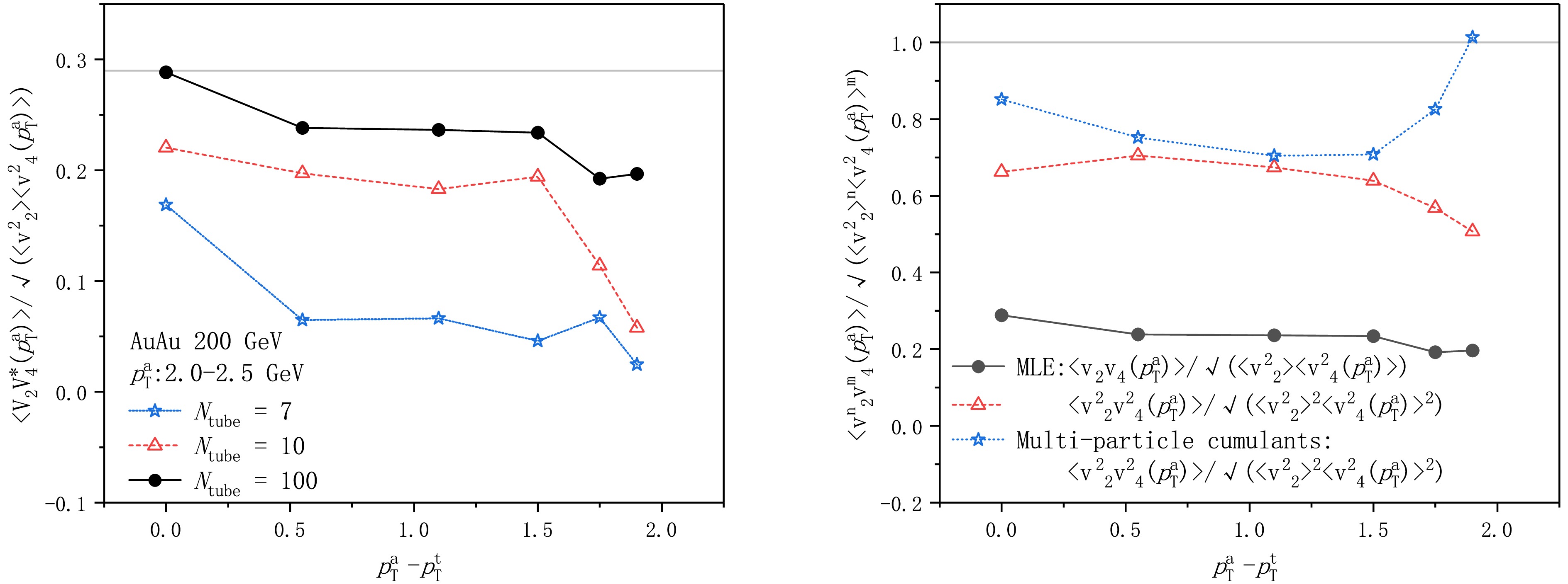

Figure 5.  (color online) Mixed harmonic factorization ratios as functions of $ p^{\rm a}_{\rm T}-p^{\rm t}_{\rm T} $ for the peripheral tube model, where the coefficients preceding the azimuthal angles do not satisfy the condition given by Eq. (27). We consider the specific choice of $ m=4 $ and $ n=2 $. The left panel shows the results for ICs generated using different numbers of tubes. The right panel evaluates the same quantity for the IC associated with $ N_{\rm{tube}}=100 $ using various constructions in terms of the order of moments. The calculations are carried out using the MLE and multi-particle cumulant methods.

Using the MLE, we investigated the relationship between initial-state fluctuations and final-state flow anisotropies in relativistic heavy-ion collisions. By reflecting on existing results on the mostly linear relation between initial state eccentricities and final state anisotropies [28, 31], the present study proceeds further based on the observation that distinct ICs may produce almost identical momentum-space anisotropy in terms of flow harmonics [32]. In this regard, our primary focus was on evaluating how the granularity of ICs, modeled using a peripheral tube approach, impacts flow factorization, a more sensitive probe compared to traditional flow harmonics. Specifically, while differential flow harmonics, such as $ v_2 $ and $ v_3 $, showed minimal sensitivity to changes in the number and configuration of tubes, the flow factorization ratio exhibited substantial variation, highlighting its potential as an effective observable for uncovering detailed information about the initial state. By employing the MLE, we extracted some specific mix-order correlators that are otherwise challenging to access, and the results showed distinct differences compared to standard techniques. We understand that the primary reason for the difference in higher-order factorization ratios between MLE and multiparticle cumulants originates from the minute difference in their definitions. The MLE is an asymptotically normal and unbiased statistical estimator with equivariance properties. While widely employed in flow analysis, multiparticle cumulant applications often involve using higher moments of the particle distribution function to estimate lower moments (cf. $ v_2\{2\} \equiv \sqrt{\widehat{v_2^2}} $). This subtle difference manifests more strongly in higher-order factorization ratios, demonstrating their sensitivity to initial-state granularity. From a theoretical perspective, the present findings require further consolidation, for instance, through systematic studies with different transport models and initial conditions. Empirically, the observed sensitivity motivates additional experimental analysis of these higher-order quantities, besides the standard flow harmonics and conventional flow factorization ratios, while employing alternative methods. We emphasize the potential of this approach to extract physically meaningful information and provide new insights into the initial conditions of heavy-ion nuclear collisions.

In this study, small-scale fluctuations were implemented in our model using high-energy peripheral tubes. As a result, it was observed that different configurations can lead to similar eccentricities $ \epsilon_n $ and, consequently, similar collective flows $ v_n $. This may explain why small-scale fluctuations are effectively averaged, resulting in comparable flow harmonics while producing more distinct high-order mixed-harmonic correlators and factorization ratios. From another perspective, the original motivation for the peripheral tube model was to attribute the observed particle correlations, known as the ''ridge'' and ''shoulder,'' to local small-scale fluctuations rather than larger-scale eccentricity. Our results indicate that higher-order correlators are better candidates than collective flows to discriminate between different models.

The present study further generalizes our initial proposal [60, 69] to a more specific subject. A primary challenge of the approach is its computational cost. Specifically, for a given event of multiplicity M, the computational time spent evaluating the N-particle cumulant is proportional to the number of distinct N-tuples. In practice, this can be reduced from $ O(M^N) $ to $ O(M) $ by removing redundancy through explicit enumeration of all possible combinations. For the MLE approach, the computational cost is dominated by the large dimension D of the parameter space θ when searching for the extremum of a high-dimensional function. Typically, it increases geometrically with D (specifically $ O(r^D) $ per iteration), where r is inversely proportional to the desired precision. For each iteration, the likelihood function must be evaluated while considering all particles. Through an appropriate numerical algorithm, our findings show that extending this approach to differential flow and particle correlators remains computationally feasible. Moreover, the MLE provides a more nuanced understanding of flow factorization and its dependence on initial-state granularity. As an asymptotically normal estimator, the MLE is robust and flexible, offering a new approach for analyzing complex multi-particle correlations. In particular, its implementation does not rely on constructing particle pairs or tuples to cancel event planes, leading to much broader applicability. Moreover, compared with the standard methods, it is more flexible to deal with scenarios where a template is not known prior to the analysis. This feature indicates a promising aspect of flow analysis that the MLE can be applied to. In this regard, applying the proposed approach to existing data would be rather interesting. Specifically, it would be pertinent to compare the results from data analysis against those obtained using more realistic event generators, such as IP-Glasma. However, some initial attempts to analyze the CMS open data were unsuccessful due to the lack of statistics (owing to a cut at low transverse momenta). We plan to continue exploring this topic in future studies.

We are thankful for enlightening discussions with Sandra Padula, Takeshi Kodama, and Yogiro Hama.