1+1 dimensional relativistic viscous non-resistive magnetohydrodynamics with longitudinal boost invariance

Heavy-ion collisions offer a unique opportunity to explore the properties of hot, dense nuclear matter - quark-gluon plasma (QGP)- created at RHIC and LHC [1, 2]. Recent research has revealed that these collisions generate extremely strong magnetic fields, ranging from 10¹⁸ to 10¹⁹ Gauss, due to the rapid motion of positively charged spectators [3−5]. These intense magnetic fields are expected to significantly influence the QGP dynamics [5−12]. The combination of strong magnetic fields and quantum anomalies can induce specialized transport phenomena known as anomalous transports. One such phenomenon is the chiral magnetic effect (CME) [13−22], which predicts charge separation in a chirality-imbalanced medium. Additionally, a chiral current can be induced by the magnetic field, leading to the chiral separation effect (CSE) [23, 24]. Together, these effects are expected to generate a density wave known as the "chiral magnetic wave" (CMW), which may disrupt the elliptic flow degeneracy between $ \pi^{\pm} $ [25]. Over the past decade, experimental collaborations at RHIC and LHC have made significant efforts to detect signals of the CME, CSE, and CMW, attracting considerable attention in studying hot, dense nuclear matter under strong magnetic fields [26−32]. However, it is still a challenge to extract the signals from the huge backgrounds caused by the collective flows.

The evolution of the QGP, primarily driven by pressure gradients, has been well-described by relativistic hydrodynamic, explaining experimentally measured harmonic flow and global polarization observed in non-central nucleus-nucleus collisions [33−46]. To fully understand the effects of strong magnetic fields on the QGP, solving the (3+1)-dimensional relativistic magnetohydrodynamics (MHD) equations is necessary [47−49], as they account for the magnetic field's dynamic coupling with the QGP fluid. Lattice-QCD calculation indicates that the QGP has a finite temperature-dependent electrical conductivity ($ \sigma_{el} $) [50, 51]. However, the interaction of the initial magnetic field with the QGP, as well as its subsequent evolution, remains unclear and is currently under active investigation [52−55]. The relative significance of an external magnetic field on fluid evolution can be evaluated using the dimensionless ratio $ \sigma \equiv B^{2}/T^{4} $, which compares magnetic-field energy density to QGP temperature. When $ \sigma>1 $, the magnetic field's influence on fluid evolution becomes substantial and must be considered [56−58].

In recent works, the influence of electromagnetic fields on the quark-gluon plasma (QGP) fluid in special relativistic systems has been investigated within the hydrodynamic framework [59]. Previous studies examined the 1+1 dimensional flow using the longitudinally boost-invariant Bjorken flow model within the MHD framework without dissipative effect [56−58, 60]. These studies incorporated a transverse and time-dependent homogeneous magnetic field while neglecting dissipative effects such as viscosity and thermal conduction. Notably, in ideal MHD, the energy density evolution follows the same decay rate as the Bjorken flow, attributed to the "frozen-flux theorem" [56]. Later, nonzero magnetization was introduced into the MHD framework [57], the longitudinal expansion effects were analyzed [61, 62], and self-similar rotating solutions were derived within the context of MHD [63].

Various studies have also analyzed the stability and causality of relativistic dissipative fluid dynamics within the frameworks of both standard and modified Israel-Stewart (IS) theories, in the presence of a magnetic field [64−68]. It has been shown that a straightforward extension of non-relativistic viscous fluid formulations (also known as Navier-Stokes theory) to the relativistic regime leads to acausal and linearly unstable behavior. These issues were subsequently addressed using the IS theory, which provides a causal and stable second-order formalism. These studies have systematically enhanced understanding of relativistic non-resistive magnetohydrodynamics (MHD).

In this study, we extend previous work by incorporating shear viscosity into the MHD equations within the Azwinndini-Bjorken viscous flow framework [69, 70], and solve them both analytically and numerically. Starting from the 1+1 dimensional relativistic non-resistive MHD [64], which includes shear viscosity and a magnetic field, we derive a series of novel solutions for non-resistive MHD. Our results indicate that for small, power-law evolving magnetic fields, the analytical solutions remain stable and demonstrate that both the magnetic field and shear viscosity contribute to fluid heating, with an early temperature peak that aligns with numerical findings. In the context of the second-order (Israel-Stewart) theory, we find that the combined presence of a magnetic field and shear viscosity leads to a slower cooling rate of the fluid temperature. Furthermore, we emphasize that our assumptions and solutions are not only straightforward but also readily adaptable to other MHD studies.

This paper is organized as follows. In Sec. II, we introduce the MHD framework with dissipative effects. In Sec. III, we present solutions for MHD based on first-order (NS) theory. In Sec. IV, we show the results for MHD in the presence of second-order (IS) theory. Finally, we summarize and conclude in the Sec. V. Throughout this study, $ u^{\mu}=\gamma\left(1,\overrightarrow{\boldsymbol{v}}\right) $ is the four-velocity field that satisfies $ u^{\mu}u_{\mu}=1 $ and the spatial projection operator $ \Delta^{\mu\nu}=g^{\mu\nu}-u^{\mu}u^{\nu} $ is defined using the Minkowski metric $ g^{\mu\nu}={\rm{diag}}\left(1,-1,-1,-1\right) $. It is note-worthy that the orthogonality relation $ \Delta^{\mu\nu}u_{\nu}=0 $ is satisfied.

In this work, we consider the causal second order theory for relativistic fluids by Israel-Stewart (IS) in the presence of a magnetic field, as given in Refs. [64, 71]. The total energy-momentum tensor of the viscous fluid is expressed as

where $ \varepsilon $ and p are the energy density and pressure, respectively; $ u^{\mu} $ is the four velocity field; and $ \pi^{\mu\nu} $ and $ \Pi $ are the shear viscous tensor and bulk viscous pressure, respectively. The magnetic field and electric field four vectors are

which satisfies $ u^{\mu}E_{\mu}=0 $ and $ u^{\mu}B_{\mu}=0 $ meaning that both $ E^{\mu} $ and $ B^{\mu} $ are spacelike. The modulus $ B^{\mu}B_{\mu}=-B^{2} $ and $ E^{\mu}E_{\mu}=-E^{2} $. Here, $ \epsilon^{\mu\nu\alpha\beta} $ is the Levi-Civita tensor satisfying $ \epsilon^{0123}=-\epsilon_{0123}=+1 $, $ F^{\mu\nu} $ is the Faraday tensor satisfying $ F^{\mu\nu}=(\partial^{\mu}A^{\nu}-\partial^{\nu}A^{\mu}) $. In the non-resistance limit, the electrical conductivity $ \sigma_{el} $ is infinite. In this limit, in order to keep the electric charge current $ j^{\mu}=\sigma_{el}E^{\mu} $ be finite, we assume the $ E^{\mu}\rightarrow 0 $. Then, the relevant Maxwell's equations which govern the evolution of magnetic fields in the fluid is $ \partial_{\nu}(B^{\mu}u^{\nu}-B^{\nu}u^{\mu})=0 $. Thus, the energy-momentum tensor simplifies as shown in Refs. [56, 64]

The space-time evolution of the fluid and electric-magnetic fields are described by the energy-momentum conservation,

To close the system of equations, we must choose the Equation of State (EoS) for the thermodynamic quantities. In the hot limit with high temperature, we assume a conformal fluid such that $ \varepsilon=3 p $, where $ c_{s}^{2}=1/3 $. For simplicity, we neglect the magnetization of the QGP [57], which implies isotropic pressure and no modification of the Equation of State (EoS) of the fluid due to magnetic field.

Since we assume longitudinal boost invariance for the fluid, it is convenient to introduce Milne coordinates, defined as $ t=\tau \cosh\eta_{s} $ and $ z=\tau\sinh\eta_{s} $, where $ \tau=\sqrt{t^{2}-z^{2}} $ is the proper time and $ \eta_{s}=0.5\ln[(t+z)/(t-z)] $ is the space-time rapidity. The fluid velocity can be expressed as

where $ \gamma=\cosh\eta_{s} $ is the Lorentz contraction factor.

Following the Refs. [56, 57, 61, 64], we consider that a simple homogeneous magnetic field obeys a power-law decay in proper time, as follow:

where a is the decay constant and $ a>0 $, $ \tau_0 $ is the initial proper time, and $ B_{0}\equiv B(\tau_{0}) $ is the initial magnetic field strength .

The energy conservation equation is derived by projecting the energy-momentum conservation law $ \partial_{\mu}T^{\mu\nu}=0 $ along the fluid four-velocity $ u_\mu $. In the Landau-Lifshitz frame, one obtains

where $ D=u\cdot \partial=\partial/\partial\tau $, $ \theta\equiv\partial_{\mu}u^{\mu}=\nabla_{\mu}u^{\mu}=\frac{1}{\tau} $ is the expansion factor and $ \pi=\pi^{00}-\pi^{33} $ [69, 70].

Similarly, the projection of the energy-momentum equation onto the direction orthogonal to $ u^{\mu} $,

yields the momentum-conservation equation

where $ \nabla^{\mu}=\Delta^{\mu\nu}\partial_{\nu} $ is the gradient operator. The last three terms vanish due to longitudinal boost invariance and $ u^{x}=u^{y}=0 $ in transverse direction [56, 70]. Note that for $ \mu=\eta_{s} $, it reads

thus indicating that all thermodynamical variables depend only on $ \tau $ and are otherwise uniform in space. Since the velocities in the $ x $- and $ y $-directions are initially zero, they remain zero at later times.

Since we fouce on the non-resistive viscous hydrodynamics, the second order Israel-Stewart (IS) theory treats viscous stresses $ \Pi $, $ \pi^{\mu\nu} $ as independent dynamical variables. Their evolution equations are given by (e.g., see Ref. [70]),

where the relaxation times $ \tau_{\Pi} $ and $ \tau_{\pi} $ are

Here, $ \zeta $ and $ \eta $ are the bulk and shear viscosity coefficients, respectively. $ \beta_{0} $ and $ \beta_{2} $ are the transport coefficients. In the final term of Eq. (12), $ \widetilde{\Delta}^{\mu\nu}=\Delta^{\mu\nu} $ for $ 0\leq\mu $, $ \nu\leq $1, and is zero otherwise (due to the fact that there is only one non-vanishing spatial component in the four-velocity).

For convenience, some useful equations and relations of thermodynamics can be written as [70]:

Here, $ \tilde{T} $ is the normalized, dimensionless temperature, and $ T_{0} $ is the temperature at the initial proper time $ \tau_{0} $. In order to more effectively isolate and highlight the heating processes, we employ uniform normalization conditions $ T_{0}=T(\tau_{0})=0.65 $ GeV, $ \tau_{0}=0.6 $ fm/c, and $ \tilde{T} $($ \tau_{0} $) = 1 for all cases. The pre-$ \tau_{0} $ solutions ($ \tau<\tau_0 $) are analytically continued to expose solution branch structure, an essential step for analyzing the non-monotonic $ \tau- $dependence that emerges under finite magnetic field and viscosity.

is a constant determined by the number of quark flavors and the number of gluon colors [70], s is the entropy density, and

Here, $ N_{f} $ is the number of quark flavors, taken as 3, and $ \alpha_{s} $ is the strong fine structure constant, taken in the range of 0.4−0.5 [70].

For a conformal fluid (i.e., a system of massless particles), the bulk viscosity $ \zeta=0 $ since the bulk viscosity does not apply to such systems [70]. Accordingly, we omitted the bulk viscosity contribution in the present work.

Let us begin by examining the 1+1 dimensional ideal MHD flow (Victor-Bjorken flow [56]), starting from Eq. (7). By neglecting the contribution from shear viscosity, the energy conservation equation can be written as

For convenience, we define the parameter $ \epsilon_{1}=\dfrac{(a-1)\sigma}{12 a_{1}} $, which depends on the strength parameter $ \sigma $ and decay exponent a of the magnetic field. With this definition, the energy conservation equation Eq. (17) is simplified to

The solution of Eq. (18) is

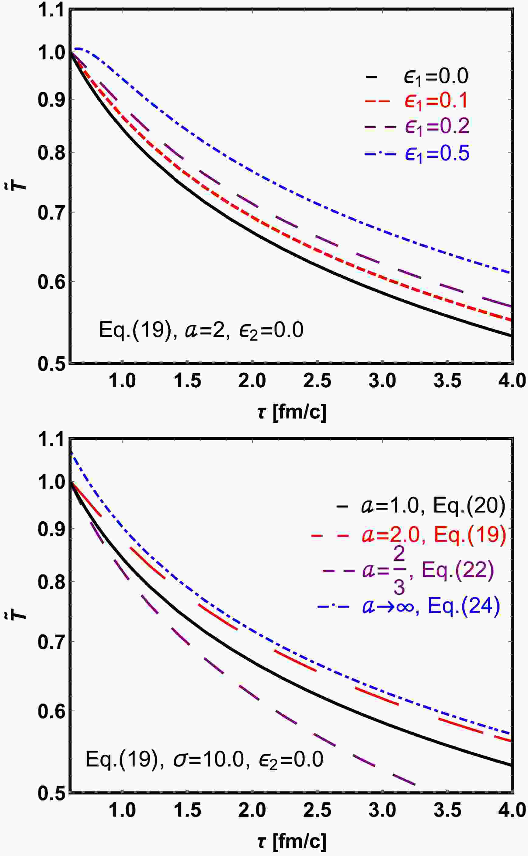
In the upper panel of Fig. 1, we plot the normalized dimensionless temperature $ \tilde{T} $ as a function of proper time $ \tau $ for $ a=2 $, considering different values of the magnetic field parameter $ \epsilon_{1} $with initial proper time $ \tau_{0}=0.6 $ fm/c. We observe that for positive $ \epsilon_{1} $ (corresponding to $ a>1 $), the normalized temperature $ \tilde{T} $ decays more slowly as $ \epsilon_{1} $ increases. This is because the energy density is "heated up" by the rapid decay of the magnetic field [56]. Additionally, a larger initial magnetic field (determined by $ \sigma $) leads to a slower decay of $ \tilde{T} $.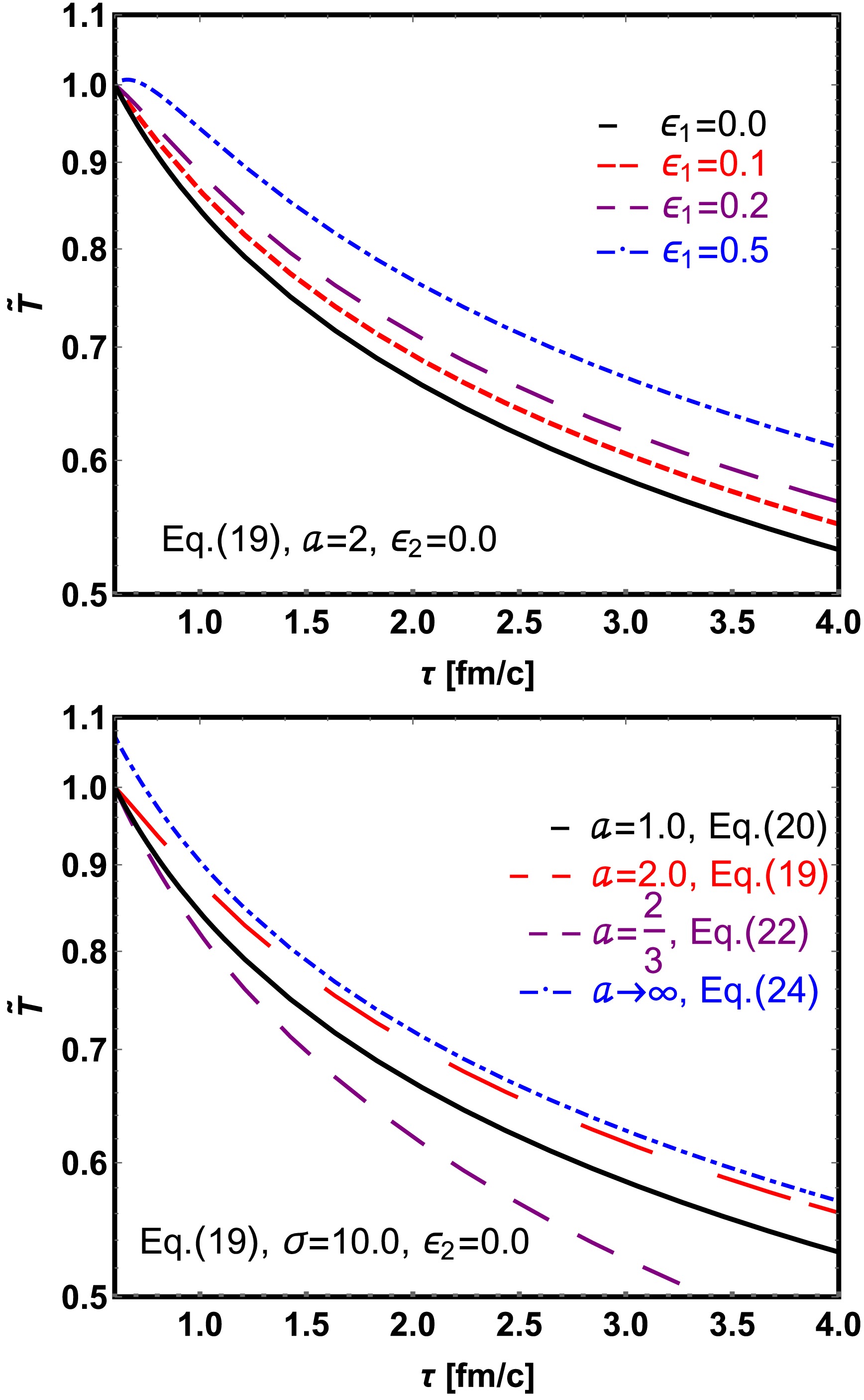

Figure 1.  (color online) Evolution of normalized temperature $ \tilde{T}=T/T_{0} $ for a magnetic field as a function of proper time $ \tau $for varying initial magnetic field (upper panel) and different values of magnetic field decay parameter a (lower panel).

We observe that Eq. (19) exhibits divergent behavior at different values of a, which determine the strength of the magnetic field. To illustrate this, we present the following solutions under specific limits:

Case-A For $ a = 1 $, we have $ \epsilon_1\equiv 0 $, which indicates the limit of infinite conductivity (or the ideal MHD limit), and thus of maximal magnetic induction. We obtain a solution of the ideal MHD; the solution type is as the same as the Victor-Bjorken flow [56],

Case-B In the limit $ a \rightarrow \frac{2}{3} $, we find

After collecting terms, the solution for $ a \rightarrow \dfrac{2}{3} $ is

For $ \tau>\tau_{0} $, the logarithmic term is negative, reducing $ \tilde{T} $ and leading to a faster temperature decrease (as shown in Fig. 1, lower panel, magenta line).

Case-C In the limit $ a \rightarrow \infty $ and $ \tau>\tau_{0} $, we find

This, results in the solution

One finds a super-fast decay of the magnetic field (as $ a \rightarrow \infty $) results to a slow decay of temperature and poses an upper limit (see Fig. 1, lower panel, purple line). This a-dependent magnetic field behavior is partly consistent with existing magnetic field evolution models, particularly for $ a\geq1 $ regimes.

In this section, we present a well-developed solution for first-order Navier-Stokes viscous flow (Azwinndini-Bjorken flow) [69]. Starting from the energy conservation equation (Eq. (7)) and by setting the magnetic field contribution to zero ($ \epsilon_{1}=0 $), we obtain

where $ \pi=\dfrac{4}{3}\dfrac{\eta}{\tau} $, $ \Pi=\zeta \dfrac{1}{\tau} $, $ \eta=b_{1}T^{3} $, and $ \zeta=b_{2}T^{3} $. For simplicity, we let $ \epsilon_{2}=\dfrac{1}{T_{0}}\dfrac{b_{1}}{9 a_{1}}=\dfrac{4}{9T_{0}}\dfrac{\eta}{s} $, where bulk viscosity coefficient $ \zeta=0 $; then, Eq. (25) can be written as

The solution of above Eq. (26) is

This solution type is as same as the Azwinndini-Bjorken solution [70]. Note that a nonvanishing shear viscosity parameter $ \epsilon_{2} $ makes the temperature cooling rate smaller.

In Fig. 2, we present the normalized dimensionless temperature $ \tilde{T} $ as a function of proper time $ \tau $, considering various shear viscosity. We find with a positive shear viscosity, while $ \epsilon_{2} $ increases from 0 to 2, $ \tilde{T} $ decreases more slowly compared to the ideal fluid case. Additionally, there is a peak in $ \tilde{T} $ in the case of NS approximation when $ \epsilon_{2} \neq 0 $.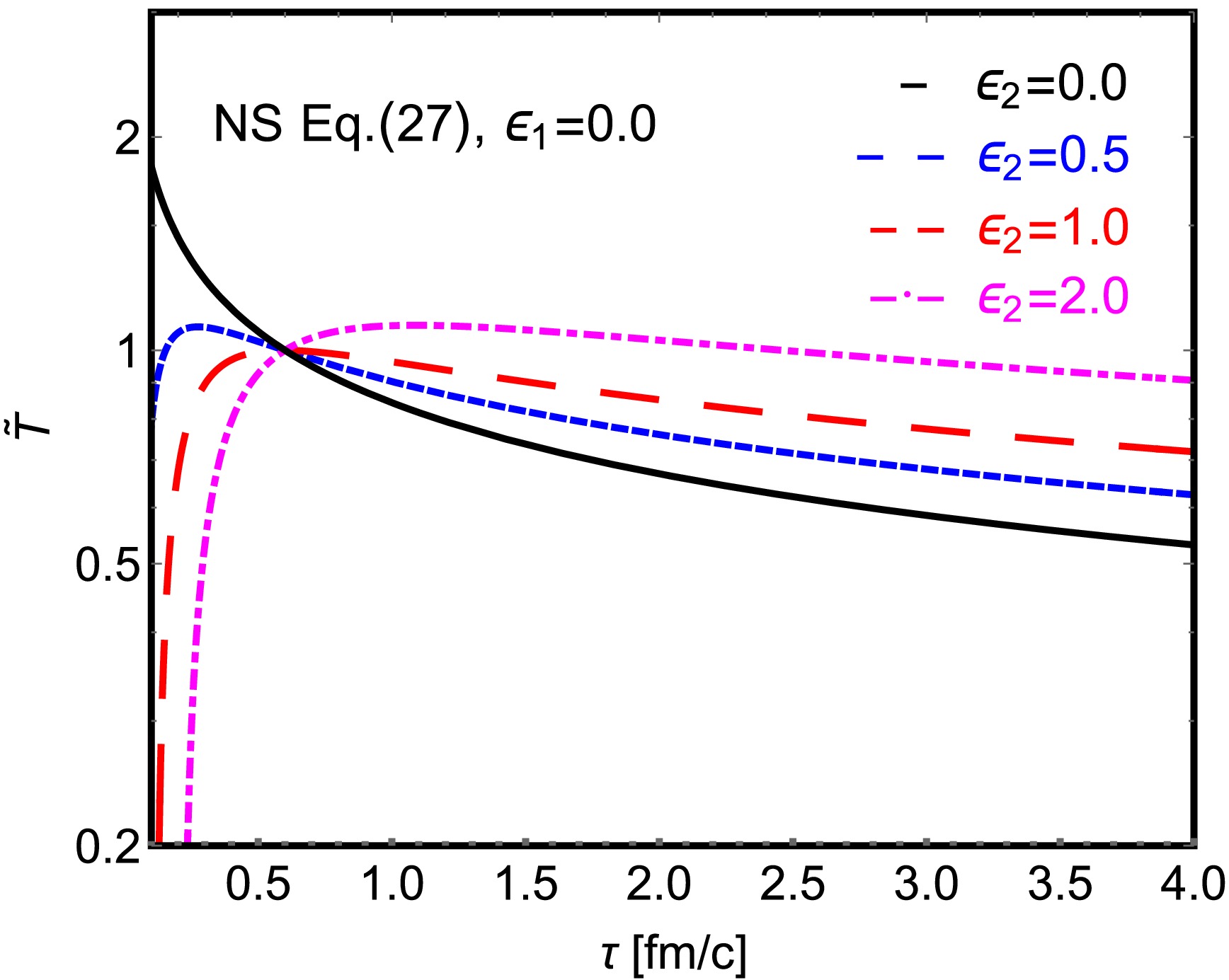

Figure 2.  (color online) Evolution of normalized temperature $ \tilde{T}=T/T_{0} $ as a function of proper time $ \tau $ for different values of shear viscosity $ \epsilon_{2} $.

In this section, we employ the nonconserved charges method [58] to solve the energy conservation equation and derive a perturbative solution that accounts for both magnetic field ($ \epsilon_{1} $) and shear viscosity ($ \epsilon_{2} $).

The energy conservation equation for a fluid with non-zero shear viscosity and non-zero magnetic field under longitudinal boost invariance takes the form:

Here, $ \epsilon_{1}=\dfrac{(a-1)\sigma}{12 a_{1}} $ and $ \epsilon_{2}=\dfrac{4}{9T_{0}}\dfrac{\eta}{s} $ with specific ranges [0, 0.5] and [0, 1 GeV⁻¹], respectively, ensuring perturbative validity. One cannot get the analytical solution of the above equation directly. However, a solution can be obtained using a perturbative method.

In Ref. [58], a nonconserved charge method is used to solve the equation for

where m is a constant and $ \lambda\left(\tau\right) $ is a known function. The general solution of Eq. (29) is:

where $ \tau_0 $ is the initial proper time and $ f(\tau_{0}) $ given by the initial value at $ \tau_0 $.

We first rewrite the energy conservation Eq. (28) as follow:

where $ m=\dfrac{1}{3} $ and

Using Eqs. (29)−(30), the formal solution of Eq. (31) is

with the condition $ \widetilde{T}\left(\tau_{0}\right)=1 $ and by introducing the variables

With the variables $ x\left(\tau\right) $, we have $ {\rm d}x(\tau)=x{\rm d}\lambda(\tau) $ and we can rewrite the Eq. (32) in the form of

where $ x\left(\tau_{0}\right)=1 $.

We assume the magnetic field value $ \epsilon_{1} $ as perturbation and solve them in powers of $ \epsilon_{1} $. In the order of $ \mathcal{O}\left(\epsilon_{1}^{0}\right) $, we have

then the solution of zero-order can be written as

In the first order of $ \mathcal{O}\left(\epsilon_{1}^{1}\right) $, we have

then we obtain

Here, $ \,_{2}F_{1}\left(a,b;c;z\right) $ is the hypergeometric function, $ \Gamma(z) $ is the Gamma function, and $ \,_{2}\widetilde{F}_{1}\left(a,b;c;z\right) $ is the regularized hypergeometric function.

Consequently, the perturbative solution of Eq. (28) is given by

where $ x_{1} $ is defined in Eq. (39). This solution remains stable when $ \epsilon_1 $ is small. We will prove this in the next Sec. IV.A.

In Fig. 3, we present the normalized temperature $ \widetilde{T}_{{\rm{NS}}-1} $ (given by Eq. (40)) as a function of proper time, for different initial magnetic field strengths ($ \epsilon_{1} $) and a fixed shear viscosity ($ \epsilon_{2}=1 $). The magnetic field decay parameter is set to $ a=2 $, and the initial proper time is $ \tau_{0}=0.6 $ fm/c. We observe that as $ \epsilon_{1} $ increases from 0.05 to 0.2, the temperature decreases more slowly compared to the ideal MHD case. Furthermore, for non-zero magnetic fields, the fluid absorbs energy in excess of the decay caused by the expansion, and leads to a peak for proper times $ \tau<0.6 $ fm/c [56].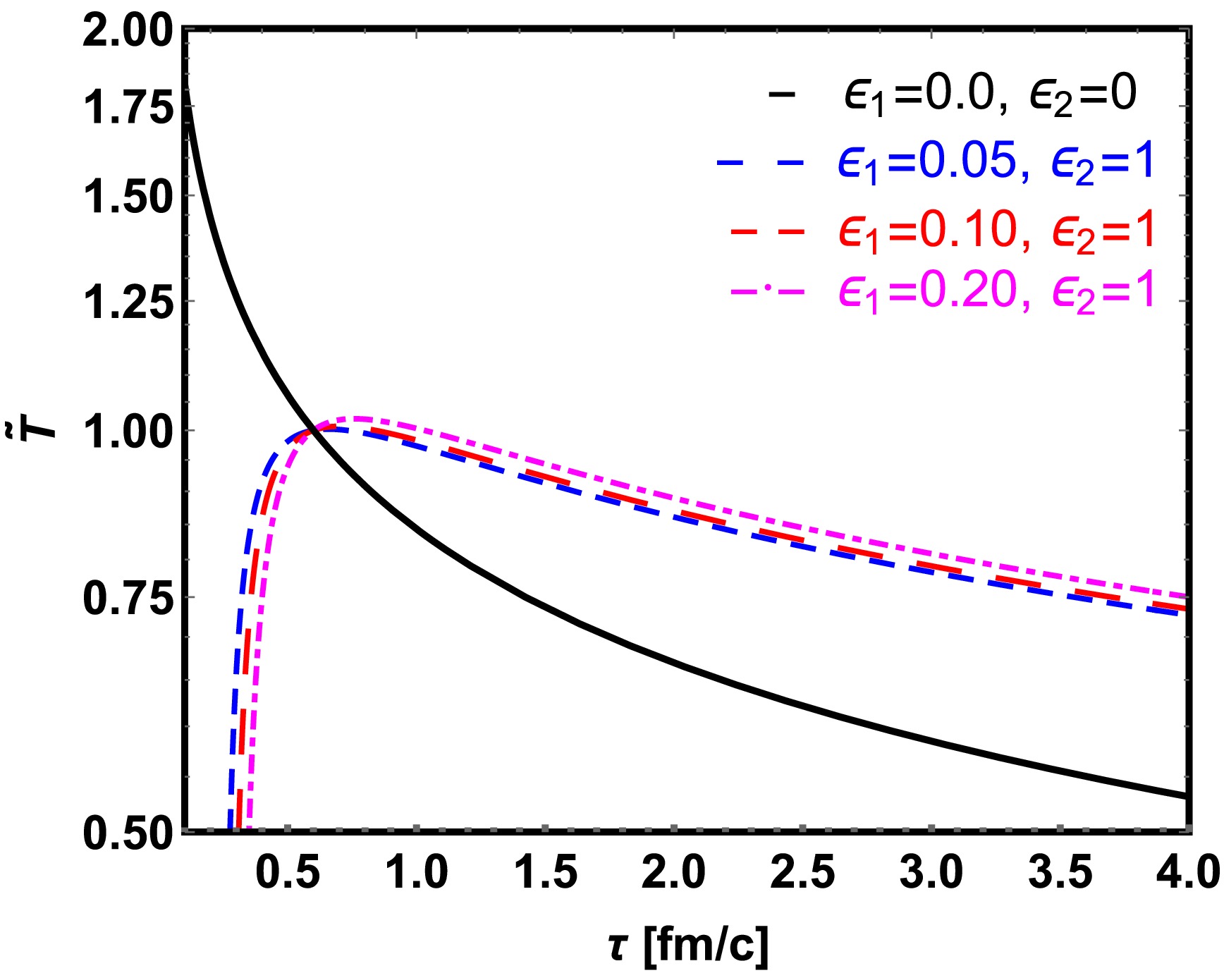

Figure 3.  (color online) Evolution of the normalized temperature $ \widetilde{T}_{{\rm{NS}}-1} $ (Eq. (40)) as a function of proper time $ \tau $ for varying initial magnetic field ($ \epsilon_{1} $), with a fixed shear viscosity value $ \epsilon_{2}=1 $, compared to the ideal MHD. The magnetic field decay parameter is $ a=2 $.

In the previous subsection-III.C, we introduced a perturbative method that can be utilized to derive an analytical solution for the NS approximation of viscous fluid dynamical equations under the assumption that the magnetic field is small ($ \epsilon_{1} $ being a small parameter). In this section, we present another perturbative solution for viscous non-resistive MHD flow within the NS approximation, assuming that both $ \epsilon_{1} $ and $ \epsilon_{2} $ are small parameters.

The energy conservation equation (Eq. (28)) for viscous MHD flow under the NS approximation is

Here, we assume that $ \epsilon_{1} $ is a small parameter. To the linear order in $ \epsilon_{1} $, the temperature $ \tilde{T} $ can be expressed as

Substituting Eq. (42) into Eq. (41), we obtain

For simplicity, we ignore terms higher than $ \mathcal{O}(\epsilon_{1}^{2}) $. Consequently, Eq. (43) reduces to

By combining the like terms in Eq. (44), we obtain

The analytical solution to the first equation in Eq. (45) is

Putting $ \tilde{T_{0}} $ into the second equation of Eq. (45), we arrive at

To obtain an analytical solution of Eq. (47), we approximate $ \tilde{T}_{0}^{3}(1+3\epsilon_{1} \tilde{T}_{0}/\tilde{T}_{1})\approx \tilde{T_{0}}^{3}\approx(\tau_{0}/\tau $), where $ \epsilon_{1} $ and $ \epsilon_{2} $ are small parameter. We note that this approximation introduces significant limitations, which will be discussed later in Fig. 5. Accordingly, Eq. (47) reduces to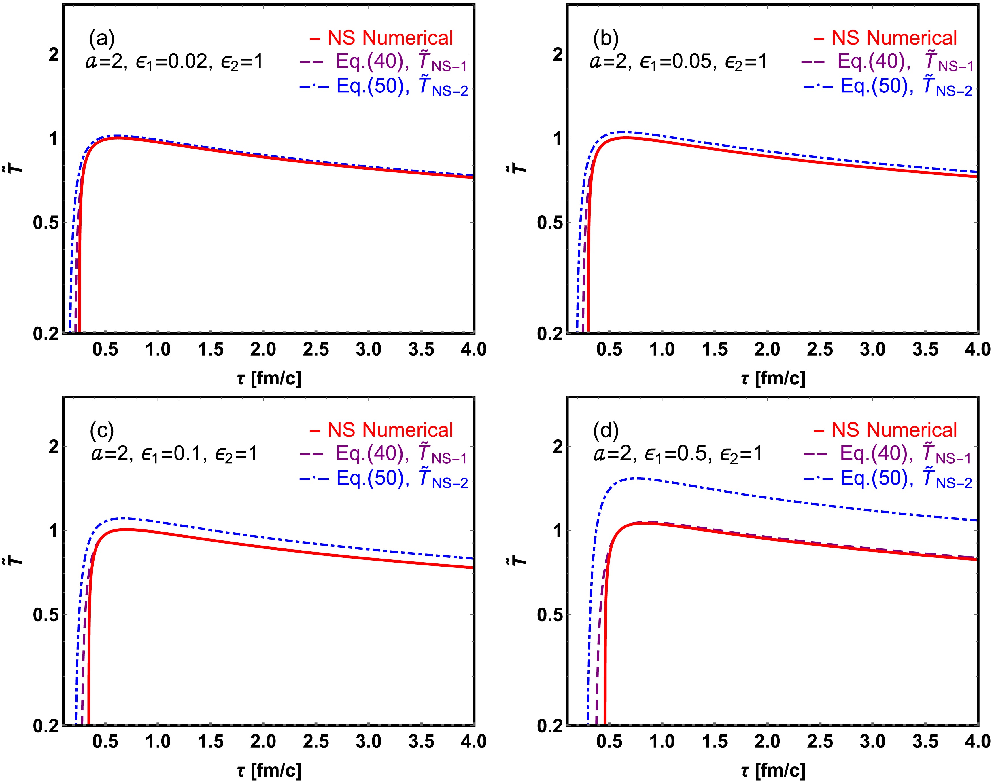

Figure 5.  (color online) Evolution of the normalized temperature $ \tilde{T} $ as a function of proper time $ \tau $, comparing two perturbative analytical solutions with numerical results. The normalized temperatures $ \tilde{T} $ are presented for various values of the magnetic field parameter $ \epsilon_{1} $, with a fixed shear viscosity ($ \epsilon_{2}=1 $) and a magnetic field decay parameter $ a=2 $.

We obtain an analytical solution of Eq. (48) as follows:

Combining the zero-order ($ \tilde{T_{0}} $) and first order terms ($ \tilde{T_{1}} $), we obtain the following perturbative analytical solution:

The above solution Eq. (50) exhibits divergent behavior for different values of the magnetic field decay parameter a. We illustrate following three particular limits as we studied in subsection-III.A.

Case-A For a=1, we obtain a solution same as the NS approximation for viscous flow.

Case-B For $ a \rightarrow \frac{2}{3} $ and $ \tau>\tau_{0} $, we obtain

Case-C For $ a \rightarrow \infty $ and $ \tau>\tau_{0} $, we assume the initial magnetic field strength parameter $ \sigma $ is a first order infinitesimal quantity, specifically $ \mathcal{O}(1/a) $, associated with a. We find that even the value of $ \epsilon_{1} $ align with the small perturbation method, but the magnetic field effect is super small, and the approximate solution regress to the viscous solution. Alternatively, if we consider $ \sigma $ as a second-order small quantity ($ \mathcal{O}(1/a^{2}) $), the magnetic field effects become too negligible to achieve our desired effect.

In Fig. 4, we present the normalized temperature as a function of proper time for various magnetic decay rates (a), with a fixed initial value of the magnetic field ($ \epsilon_{1}=0.1 $) and shear viscosity ($ \epsilon_{2}=0.2 $). One finds for $ 0<a<1 $, the third term in $ \tilde{T} $ in Eq. (52) is negative, resulting in faster decay compared to both the ideal MHD case and the $ a=1 $ case (as described in Eq. (51)). Furthermore, when $ a>1 $, the third term of $ \tilde{T} $ in Eq. (50) is always positive, results in a slower decay compared to the ideal MHD case.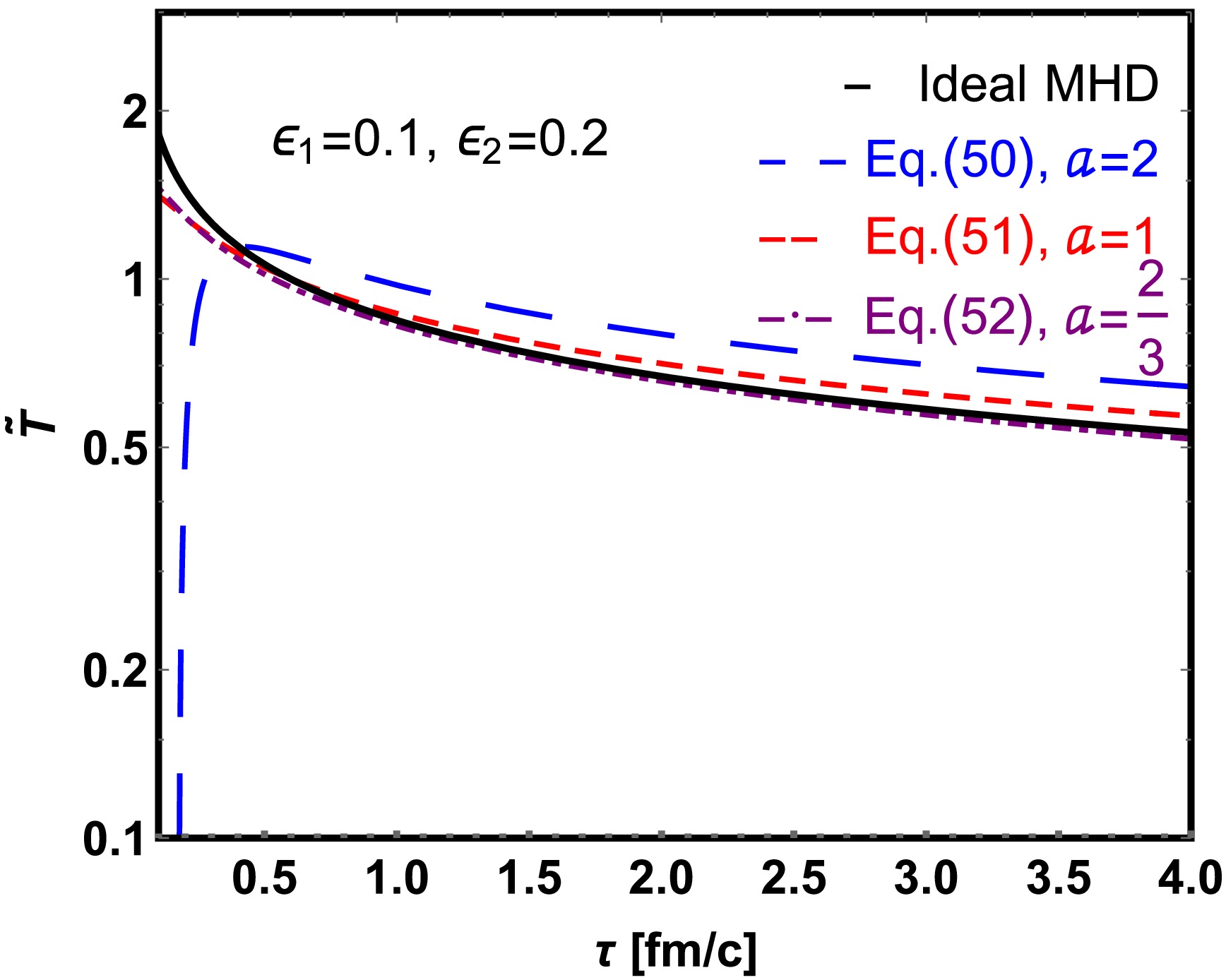

Figure 4.  (color online) Evolution of normalized temperature $ \widetilde{T}_{{\rm{NS}}-2} $ (Eqs. (50)−(52)) as a function of proper time $ \tau $ for different values of magnetic decay parameter a with fixed initial magnetic field ($ \epsilon_{1}=0.1 $) and fixed shear viscosity value ($ \epsilon_{2}=0.2 $), compared to the ideal MHD.

In this section, we present the numerical solution of viscous non-resistive magnetohydrodynamics with longitudinal boost invariance using both the first order Navier-Stokes (NS) approximation and the second order Muller-Israel-Stewart (IS) approximation.

We begin with the energy conservation equation under the first order NS approximation, expressed as

Using the initial condition $ T_{0}=0.65 $ GeV and $ \tau_{0}=0.6 $ fm/c, we obtain the numerical solution of above Eq. (53) quickly.

In Fig. 5 we present the normalized temperature $ \tilde{T} $ as a function of proper time $ \tau $ for different magnetic field $ \epsilon_{1} $, fixed shear viscosity $ \epsilon_{2} $, and compare it with the previous perturbative analytical solutions in Eqs. (40) and (50). The initial proper time sets $ \tau_{0}=0.6 $fm/c and the magethe magnetic field decay parameter a=2.

In the upper left panel of Fig. 5, with parameters $ a=2 $, $ \epsilon_{1}=0.02 $, and $ \epsilon_{2}=1 $. The initial magnetic field strength is given by $ B_{0}^{2}=0.24a_{1} T_{0}^{4} $. We observe that the perturbative analytical solution $ \tilde{T}_{{\rm{NS}}-1} $ aligns very closely with the numerical results, whereas the solution $ \tilde{T}_{{\rm{NS}}-2} $ is found to be in close to and slightly higher than the numerical solution.

In the upper right panel of Fig. 5, for the same value for $ a=2 $ but with $ \epsilon_{1}=0.05 $ and $ \epsilon_{2}=1 $, the initial strength of magnetic field is calculated as $ B_{0}^{2}=0.6a_{1} T_{0}^{4} $. Here, the solution $ \tilde{T}_{{\rm{NS}}-1} $ agrees well with the numerical results, whereas $ \tilde{T}_{{\rm{NS}}-2} $ exceeds the numerical solution by approximately 5%.

In the lower panel of Fig. 5, with the magnetic field parameter $ \epsilon_{1}=0.1 $ (left) and $ \epsilon_{1}=0.5 $ in the right panel. We find that the analytical solution $ \tilde{T}_{{\rm{NS}}-1} $ remains consistent with the numerical solution. However, $ \tilde{T}_{{\rm{NS}}-2} $ deviates significantly from the numerical solution as $ \epsilon_{1} $ grows, indicating that this second perturbative solution becomes less stable compared to the analytical solution and numerical solution.

We summarize the differences between the two perturbative solutions (Eqs. (40) and (50)) as follows: (1) When$ \epsilon_{1} $< 0.05, both analytical solutions (Eqs. (40) and (50)) align well with the numerical solution, capturing the key features of temperature evolution; (2) The solution $ \tilde{T}_{{\rm{NS}}-1} $ (Eq. (40)) remains robust for small $ \epsilon_{1} $, with minimal influence from the shear viscosity $ \epsilon_{2} $.

In the second order theory, the bulk viscous pressure $ \Pi $ and shear stress tensor $ \pi $ have to be determined from the second order transport equations. Based on Refs. [69, 70], the energy conservation equation and viscosity evolution equations can be written as:

For massless particles, the relaxation coefficient is $ \beta_{2}=3/(4p) $ and the relaxation time becomes $ \tau_{\pi} $, which is then calculated as $ \tau_{\pi}=2\eta\beta_{2} $ [70]. As discussed in previous sections, since we are considering a system of massless particles and utilizing the equation of state $ \varepsilon=3p $, this leads to the absence of bulk viscosity, and therefore, it will not be included in subsequent discussions.

Following Ref. [70], the value of initial shear stress (viscosity) $ \pi_{0} $ (defined as $ \pi_{0}=\pi^{00}_{0}-\pi_{0}^{33} $) assume to control by the initial pressure $ p_{0} $. For simplicity, we assume an initial condition where $ \pi_{0} \equiv b_{3}p_{0}=a_{1}b_{3}T_{0}^{4} $, with $ b_{3} $ being a constant. We further define a normalized fluid shear viscosity $ \tilde{\pi} $ as $ \tilde{\pi}=\pi/\pi_{0} $ and make it a dimensionless parameter. With this setup, the energy conservation equation reduces to

In addition, the shear viscosity equation reduces to

From Eqs. (57) and (58), the energy conservation equation and shear viscosity equation can be written as

We numerically solved these second order (IS) approximation fluid differential equations, Eqs. (59) and (60), using fixed initial conditions and compared the second order (IS) results with those from ideal MHD and first order (NS) theory.

In the upper panel of Fig. 6, we present the normalized temperature $ \tilde{T} $ as a function of proper time $ \tau $ for ideal MHD, first order (NS) solution and second order (IS) with a zero magnetic field. The shear viscosity $ \epsilon_{2} $ is $ \epsilon_{2}=1 $. The initial condition for $ \pi_{0} $ is $ \pi_{0}=0.1p_{0} $ where $ b_{3}=0.1 $. In this figure a comparison between the perfect fluid approximation, the first order theory, and the second order theory is clear. One finds that considering a non-zero shear viscosity makes the fluid cool down more slowly compared to the ideal MHD. Ones sees that there is a peak in $ \tilde{T} $in the first-order (NS) theory, and no such peak appears in the second-order (IS) theory.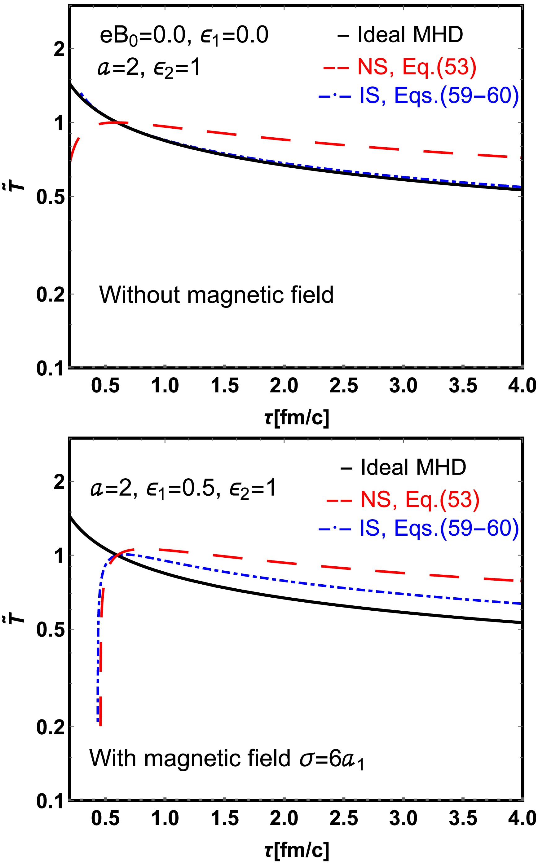

Figure 6.  (color online) Evolution of normalized temperature $ \widetilde{T} $ (Eqs. (53), (59), (60)) as a function of proper time $ \tau $, comparing results from ideal MHD, first-order (NS) theory, and second-order (IS) theory. Simulations are shown for different initial magnetic field strengths ($ \epsilon_{1} $) with a fixed shear viscosity value $ \epsilon_{2}=1 $ and magnetic field decay parameter $ a=2 $.

In the lower panel of Fig. 6, we plot the normalized temperature $ \tilde{T} $ as a function of proper time $ \tau $ under three scenarios: ideal MHD, first-order (NS) approximation, and second-order (IS) approximation, each incorporating non-zero magnetic field and shear viscosity. The specific parameters are set as follows: magnetic field decay parameter $ a=2 $, magnetic field strength parameter $ \epsilon_{1}=0.5 $, and shear viscosity parameter $ \epsilon_{2}=1 $. The initial condition for the shear stress is specified as $ \pi_{0}=0.1p_{0} $, corresponding to $ b_{3}=0.1 $. The results indicate that the presence of a magnetic field leads to a slower cooling rate of the fluid compared to the case where only shear viscosity is considered. Furthermore, both the first-order and second-order theories exhibit a peak in $ \tilde{T} $ at very early times in the system's evolution. The cooling rate of temperature in the second-order IS theory is slower than that in ideal MHD but faster than in the first-order NS theory.

In Fig. 7, we present the normalized temperature $ \tilde{T} $ as a function of proper time $ \tau $ based on the second-order (IS) theory, highlighting the influence of different initial conditions for $ \pi_{0} $. The magnetic field decay parameter $ \epsilon_{1} $ is set to $ 0.5 $ and the magnetic field decay parameter a is 2. We compare four different initial conditions for $ \pi_{0} $: $ 0.1p_{0} $, $ 0.5p_{0} $, $ 1p_{0} $ and $ 2p_{0} $, where $ p_{0} $ is the initial pressure of the fluid. We find that increasing $ \pi_{0} $ (or equivalently, increasing the coefficient $ b_{3} $) leads to a slower cooling rate, suggesting that the initial shear stress significantly impacts the thermal evolution of the fluid. Additionally, in all cases, there is a peak in $ \tilde{T} $ observed at early times, which is a characteristic of viscous non-resistive magnetohydrodynamics. This peak arises due to the non-zero magnetic field heated up the fluid, which influence the fluid's cooling behavior. In physical QGP systems, $ \pi_{0} $ is typically smaller than the pressure $ p_{0} $, as supported by both microscopic theoretical models and experimental analyses.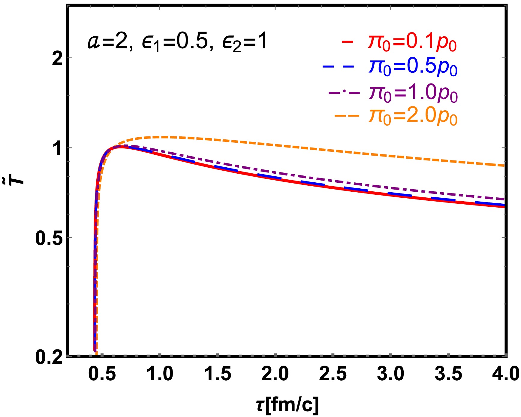

Figure 7.  (color online) Evolution of normalized temperature $ \widetilde{T} $ (59, 60) from second-order (IS) theory as a function of proper time $ \tau $ for different initial value of shear viscosity $ \pi_{0} $ with fixed initial magnetic field $ \epsilon_{1}=0.5 $, shear viscosity parameter $ \epsilon_{2}=1 $, and magnetic field decay parameter $ a=2 $.

Motivated by the exploration of strong magnetic fields and shear viscosity in relativistic heavy-ion collisions, we investigated the evolution of flow temperature in a 1+1 dimensional viscous, non-resistive magnetohydrodynamic flow with an EOS $ \varepsilon=3p $. Our idealized setup, which focuses on longitudinally boost-invariant flow with a transverse magnetic field and constant shear viscosity, yields various analytical solutions.

This work generalize the Victor-Bjorken ideal MHD flow [56, 57] and the Azwinndini-Bjorken dissipative flow [69, 70] to scenarios incorporating both non-zero shear viscosity and a magnetic field. Specifically, the analytical solution reduces to the Bjorken flow in the absence of both magnetic field and shear viscosity, to the Victor-Bjorken type solution when only a magnetic field is present, and to the Azwinndini-Bjorken solution when only shear viscosity is present. With both magnetic field and first-order (Navier-Stokes) shear viscosity, we derived two new perturbative solutions and compared them with numerical results. We also obtained numerical solutions for different initial shear stress values $ \pi_{0} $ in the second-order (Israel-Stewart) theory. Although simplified, our findings provide insights into the fluid dynamics in high energy regions.

We further analyzed cases with arbitrary shear viscosity and a small magnetic field evolving according to a power-law in proper time with exponent a. For initial magnetic field strengths ($ B^{2}_{0} $) smaller than 6$ a_{1}T^{4}_{0} $ and for proper time $ \tau > 0.6 $ fm/c, our analytical solution is stable. We observe that larger magnetic fields ($ \epsilon_{1} $) with decay parameter $ a>1 $ lead to fluid reheating, which manifests as an early-time temperature peak. The peak's magnitude depends on both the magnetic field strength and shear viscosity. At later times, the temperature asymptotically decreases that is the same as in the Azwinndini-Bjorken flow. We also consider the case where the shear viscosity and magnetic field are both small. The analytical solution in this case is consistent with the numerical results while the magnetic field is pretty small ($ \epsilon_{1}<0.02 $), but deviates to become 5% greater than the numerical results while $ \epsilon_{1}>0.05 $.

Finally, we presented numerical results for the second-order (Israel-Stewart) theory. We found that the presence of magnetic field and shear viscosity leads to a slower cooling rate of the fluid temperature compared to the case with shear viscosity alone. Moreover, the initial shear stress $ \pi_{0} $ in the longitudinal boost-invariant fluid plays a significant role in determining its temperature evolution.

We thank Shi Pu and Shen-Qin Feng for helpful discussions and comments.