Alpha-decay systematics and a new scaling law in heavy and superheavy nuclei

Alpha radioactivity has long served as a cornerstone in nuclear physics, dating back to the discovery of radioactivity by Henri Becquerel in 1896 [1, 2]. A major theoretical breakthrough occurred in 1928, when Gamow [3] and, independently, Condon and Gurney [4] introduced the quantum tunneling mechanism to explain α-decay, marking the first application of quantum mechanics to nuclear phenomena. Since then, α-decay has remained a vital probe in understanding the structural and energetic properties of atomic nuclei, particularly in the heavy and superheavy regions.

The utility of α-decay lies in its high sensitivity to nuclear structure. Decay half-lives, $ Q_\alpha $ values, penetrability, and the α -preformation factor all reflect underlying shell effects, deformation, and pairing correlations [5, 6]. Of particular importance is the role of α-decay in identifying shell and sub-shell closures, both spherical and deformed. Significant variations in α-decay half-lives or $ Q_\alpha $ values often correspond to enhanced nuclear binding, signaling the presence of magic numbers. In this context, α-decay has proven effective in confirming well-known closures at $ N = 126 $ and $ Z = 82 $, as well as in probing the debated magicity of predicted closures, such as $ N = 184 $ in superheavy nuclei [7−10]. In addition to spherical closures, anomalies in decay systematics have also been linked to deformed shell gaps, as identified in Nilsson-level schemes and mean-field models [11, 12]. Such signatures provide insights into shape coexistence and nuclear deformation, reinforcing the status of α-decay as a structural fingerprint.

From a theoretical perspective, the semiclassical Wentzel-Kramers-Brillouin (WKB) approximation remains one of the most widely used frameworks for modeling α-decay as quantum tunneling. When paired with fission-like treatments, α-decay is modeled as the emission of a preformed cluster through a potential barrier, often constructed using the double-folding model (DFM). The DFM derives the interaction potential microscopically by folding the density distributions of the α-particle and daughter nucleus with an effective nucleon-nucleon interaction [13−15], and it has been successfully applied in both nuclear reaction and decay contexts [16]. Refinements such as the Langer correction [17] and Bohr-Sommerfeld quantization condition [18] have improved the accuracy of the model in predicting lifetimes and decay rates.

Equally important to potential construction are the nuclear density distributions themselves, which serve as inputs to the DFM. Traditional treatments often adopt a two-parameter Fermi (2pF) distribution with a radius scaling as $ A^{1/3} $ [19−22]. However, more recent approaches have allowed for deviations from this idealized form, including central density depression, fluctuations, and surface asymmetry [23−26], which are especially relevant in exotic and superheavy nuclei.

Alongside microscopic methods, empirical and semi-empirical formulas have played a key role in the systematic study of α-decay. The Viola-Seaborg (VS) formula [27] and its various refinements remain among the most widely used approaches for estimating α-decay half-lives, employing correlations based on Z and $ Q_\alpha $. Royer [28] and others have further optimized such relations using composite variables such as $ Z Q_\alpha^{-1/2} $ or $ A^{1/6} Z Q_\alpha^{-1/2} $ to fit large datasets of even-even and odd nuclei. The Universal Decay Law (UDL) introduced by Qi et al. [29] aimed to unify α and cluster decays into a single framework, while Sobiczewski and Parkhomenko [30] proposed simplified expressions tailored to superheavy systems. Poenaru et al. [31] introduced a universal decay curve that captures global systematics across the nuclear chart. These studies consistently demonstrate that deviations from fitted trends often reflect underlying nuclear structure effects, including magic numbers and deformation.

Notably, multiple studies have attempted to recast α-decay systematics into linearized forms involving composite variables such as $ Z^\alpha Q_\alpha^{-\beta} $, seeking both theoretical simplicity and predictive robustness [32−34]. Such parametrizations aim to isolate the influence of Coulomb and tunneling effects while exposing residual structural signals, often linked to shell closures, as localized deviations. By analyzing decay properties as a function of these reduced variables, researchers have identified both global trends and local anomalies, further enhancing the diagnostic power of α-decay studies.

Despite these developments, challenges remain in achieving reliable decay predictions in the heaviest nuclei, particularly due to sparse experimental data and model uncertainties. Continued refinement of both microscopic potential models and empirical systematics is therefore necessary to probe shell effects, constrain theoretical models, and guide experimental searches for new elements and isotopes.

In this context, α-decay continues to offer a uniquely sensitive and informative window into nuclear structure. Its strong dependence on nuclear binding, shell effects, and deformation makes it not only a decay mode but also a probe capable of illuminating the landscape of magicity in both known and unexplored regions of the nuclear chart. The present study builds upon the theoretical and empirical foundations outlined above to explore the behavior of α-decay in selected isotopic chains of heavy and superheavy elements. By combining microscopic potential modeling with updated correlation techniques, this study aims to contribute to the ongoing effort of refining decay predictions and understanding the structural signatures embedded in α-decay observables.

In the present study, a systematic, multi-stage approach is employed to model α-decay in heavy and superheavy nuclei. The approach consists of three main components: (1) calculation of the nuclear total energy and density distributions, (2) obtaining the α-daughter interaction potential, and (3) computation of the α decay half-life. The accuracy of α-decay calculation critically depends on the Q-value, as it determines both the boundaries of the potential well where the α particle is formed and the potential barrier it must tunnel through, during the decay process [35]. Additionally, the nuclear density distribution plays a critical role, as it directly influences the interaction potential between the α-particle and the daughter nucleus [13].

In the first stage, ground-state (gs) nuclear energies are computed by minimizing the total nuclear energy across a multi-dimensional energy surface [36]. This process yields density distribution parameters, corresponding to the optimum energy, and ground-state energies, from which Q-values are derived.

In the second stage, the α -daughter interaction potential is calculated using the double folding model (DFM) [13]. This involves folding the nuclear density of the daughter nucleus (obtained in the first stage) and α-particle density with nucleon-nucleon interactions.

In the third stage, the Q-value, derived from the energy difference between parent and daughter nuclei, is combined with the α-daughter potential to compute α-decay associated probabilities and subsequently determine the half-life [37].

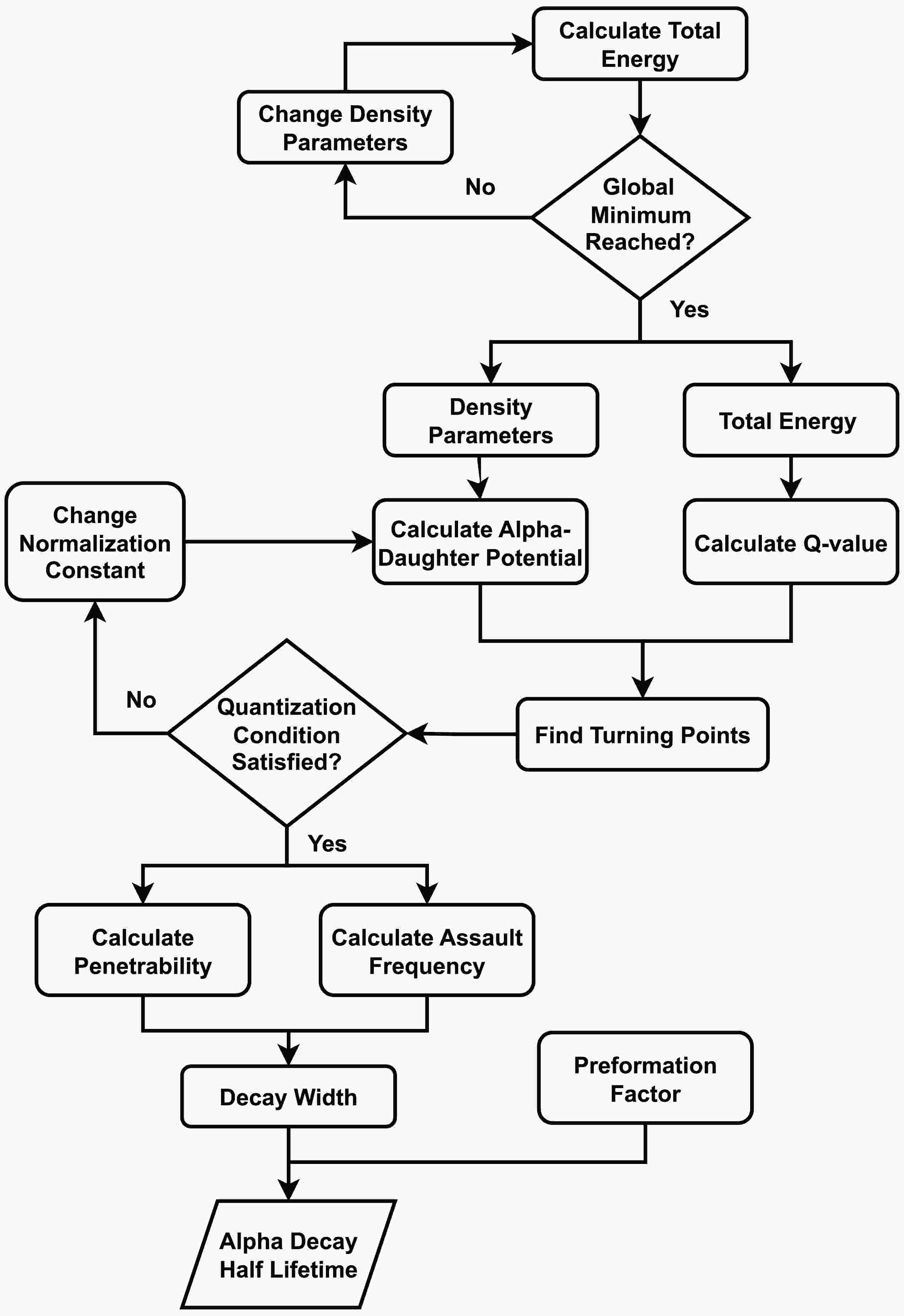
Figure 1 shows a schematic overview of the computational workflow, illustrating the sequential steps and their interdependencies. The subsequent subsections detail the theoretical framework underlying the calculations in this study, as briefly outlined above.

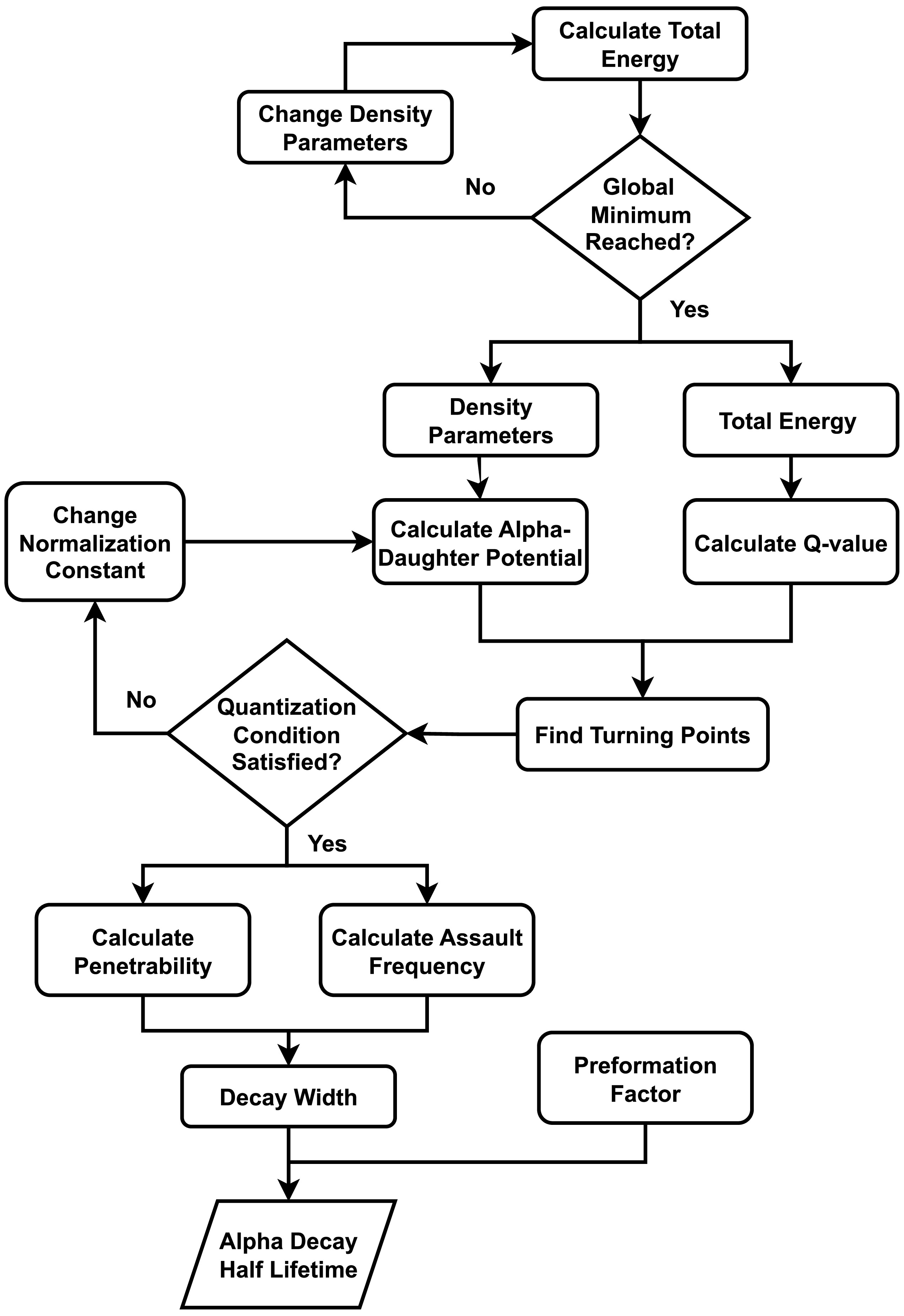
Figure 1.  Scheme of α-decay calculation overflow.

In the present study, a systematic, multi-stage approach is employed to model α-decay in heavy and superheavy nuclei. The approach consists of three main components: (1) calculation of the nuclear total energy and density distributions, (2) obtaining the α-daughter interaction potential, and (3) computation of the α decay half-life. The accuracy of α-decay calculation critically depends on the Q-value, as it determines both the boundaries of the potential well where the α particle is formed and the potential barrier it must tunnel through, during the decay process [35]. Additionally, the nuclear density distribution plays a critical role, as it directly influences the interaction potential between the α-particle and the daughter nucleus [13].

In the first stage, ground-state (gs) nuclear energies are computed by minimizing the total nuclear energy across a multi-dimensional energy surface [36]. This process yields density distribution parameters, corresponding to the optimum energy, and ground-state energies, from which Q-values are derived.

In the second stage, the α -daughter interaction potential is calculated using the double folding model (DFM) [13]. This involves folding the nuclear density of the daughter nucleus (obtained in the first stage) and α-particle density with nucleon-nucleon interactions.

In the third stage, the Q-value, derived from the energy difference between parent and daughter nuclei, is combined with the α-daughter potential to compute α-decay associated probabilities and subsequently determine the half-life [37].

Figure 1 shows a schematic overview of the computational workflow, illustrating the sequential steps and their interdependencies. The subsequent subsections detail the theoretical framework underlying the calculations in this study, as briefly outlined above.

Figure 1.  Scheme of α-decay calculation overflow.

In this study, we employed a macroscopic-microscopic model based on the Skyrme energy density functional, incorporating shell and pairing corrections to capture nuclear structure effects [38−42]. The total energy combines a smooth macroscopic component, derived from the Skyrme force [43, 44], with microscopic corrections calculated using the Strutinsky method [45] and Bardeen-Cooper-Schrieffer (BCS) formalism [46]. The energy density functional is expressed as

where $ \tau_i ({r}) $ are the kinetic energy densities for protons ($ i=p $) or neutrons ($ i=n $), $ \mathscr{H}_{\text{nuc}}({r}) $ denotes the nuclear energy density, and $ \mathscr{H}_{\text{Coul}}({r}) $ is the Coulomb energy density [47, 48]. The proton and neutron densities are modeled with a two-Parameter Fermi (2pF) function:

where $ R_i(\theta,\phi) $ is the orientation-dependent surface radius, incorporating the full set of deformation parameters, and $ a_i $ are the diffuseness values for proton and neutron distributions. This application of the Skyrme energy density functional using a two-parameter Fermi density differs from a calculation that uses the self-consistent density obtained by solving the Skyrme-Hartree-Fock equations. Consequently, the integration of the Skyrme energy functional with this phenomenological form does not include any shell effects. The central density, $ \rho_{0i} $, is determined by normalization to the total nucleon number:

The half-density surface $ R_i(\theta,\phi) $ is defined as

Hence, the Skyrme-based energy density functional can be parameterized with degrees of freedom being the set of axially symmetric deformation parameters $ \beta_{\lambda} $, where the choice $ m = 0 $ corresponds to the axial symmetry assumption and conservation of the projection of angular momentum on the symmetry axis. This choice is well suited for capturing the leading collective deformation modes in heavy and superheavy nuclei. The parametrization also includes the half-density radii $ R_{0i} $ and diffuseness $ a_i $ of both proton and neutron distributions [38−40, 49].

The shell correction is mainly attributed to the non-uniformity of the single-particle (SP) levels near the Fermi energy [41, 45]. The shell-correction energy is calculated using the well-known Strutinsky method with a deformed Woods-Saxon potential and a universal set of parameters [50−52]. The SP energy levels are obtained by diagonalizing the single-particle Hamiltonian in a deformed harmonic oscillator basis [53]. The shell correction energy is defined as the difference between the sum of the occupied SP energies, $ E_{\text{shell}} = 2 \sum \varepsilon_i $, and its smoothed counterpart, obtained using a smoothing procedure:

where $ \tilde{g}(\varepsilon) $ is the smoothed level density and $ \tilde{\lambda} $ is the corresponding smoothed Fermi level, determined by normalizing to the number of particles: $ N(P)=2 \int_{-\infty}^{\tilde{\lambda}} \tilde{g}(\varepsilon) {\rm d}\varepsilon $.

The smoothed level density $ \tilde{g}(\varepsilon) $ is obtained by folding the discrete level density $ g(\varepsilon) = \sum_i \delta(\varepsilon - \varepsilon_i) $ with a smoothing function $ f(x) $, defined as a product of a Gaussian and generalized Laguerre polynomial:

where the smoothing function is defined as follows:

where γ is the smoothing parameter and m is the order of the curvature correction polynomial. For infinite potentials such as the infinite square well, harmonic oscillator, and deformed Nilsson potentials, one can generally identify a range of the smoothing parameter γ and correction polynomial order m where the smoothed single-particle energy is uniquely defined [54, 55]. When using Eq. (6) to calculate the shell correction, it remains stable over a range $ \hbar \omega \lessapprox \gamma \lessapprox 2 \hbar \omega $ [45, 56], ensuring a well-defined result. This plateau condition holds well for harmonic oscillator and Nilsson potentials [54, 56, 57]. The smoothed level density $ \tilde{g}(\varepsilon) $ is thus obtained by averaging single-particle levels over an energy width of order $ \hbar \omega $. We use a basis of 19 axially deformed harmonic oscillator shells and a sixth-order correction polynomial, a standard choice for medium to superheavy nuclei [57, 58]. The smoothing width γ is taken as $ \gamma \gtrapprox \hbar \omega \approx 7 $–$ 10 $ MeV, where $ \hbar \omega \approx 41/A^{1/3} $ MeV [59]. Incorporating the shell correction energy using a smoothed level density to isolate quantal fluctuations beyond the mean field ensures that double counting is avoided, as we subtract the smooth component already present in the mean field from the total single-particle energy.

The pairing correction energy is treated microscopically within the Bardeen–Cooper–Schrieffer (BCS) framework [41, 46]. Analogous to the shell correction method, the residual pairing correction is defined as

where $ E_{\text{pair}} $ is the total pairing energy, and $ \tilde{E}_{\text{pair}} $ represents its smoothed counterpart based on an average single-particle distribution.

To evaluate $ E_{\text{pair}} $, we follow the standard BCS approach, solving the coupled equations for the Fermi level λ and the pairing gap Δ self-consistently. The effective strength of the pairing interaction G is defined as

Alternatively, it can be expressed in an integral form over the smoothed level density $ \tilde{g}(E) $:

where Ω is a cutoff energy defined in terms of the number of active states $ n_c $ as $ \Omega = n_c / \tilde{g}(\tilde{\lambda}) $. The occupation probabilities $ \nu_v^2 $ of the single-particle states are determined from

ensuring the conservation of particle number: $ N = 2 \sum_v \nu_v^2 $. The pairing energy is then computed as [41, 57]

while the smoothed counterpart is evaluated using

where $ \tilde{\Delta} $ is the average pairing gap [8, 45]. Both shell and pairing corrections stem from the microscopic structure of single-particle levels near the Fermi energy and are consistently derived from the same underlying mean-field potential. Accordingly, both are treated within the Strutinsky prescription, ensuring methodological consistency and compatibility between the shell and pairing effects.

The total energy surface, $ E(R_{0i}, a_i, {\beta_{\lambda}}) $, is obtained by integrating the energy density and adding the microscopic corrections, all considered at the same values of the adjustable density distribution parameters,

This total energy is optimized in multidimensional deformation space to determine the binding energy ($ BE $) and corresponding density distribution parameters. The adopted framework, which is based on a Skyrme energy density functional, is particularly suited for such multidimensional optimization techniques, which are specifically adapted here to enhance predictive accuracy. As emphasized, the model provides a computationally tractable yet physically rich formalism that enables the systematic inclusion of microscopic corrections, namely, shell effects via the Strutinsky method [42, 45] and pairing correlations through the BCS approach [46, 53]. Its flexibility supports robust parameter fitting across extended isotopic chains and facilitates consistent reproduction of α-decay trends and systematics in heavy and superheavy nuclei. Furthermore, its success in established models such as the FRDM [8, 60] and related approaches [30, 61] reinforces its reliability and relevance to the present investigation.

The Q-value for α-decay ($ Q_\alpha $) is determined by considering the binding energies of both parent (P) and daughter (D) nuclei, extracted from their respective energy surfaces,

where the binding energy of the α-particle is taken as $ BE_\alpha = 28.2957 $ MeV [62].

In this study, we employed a macroscopic-microscopic model based on the Skyrme energy density functional, incorporating shell and pairing corrections to capture nuclear structure effects [38−42]. The total energy combines a smooth macroscopic component, derived from the Skyrme force [43, 44], with microscopic corrections calculated using the Strutinsky method [45] and Bardeen-Cooper-Schrieffer (BCS) formalism [46]. The energy density functional is expressed as

where $ \tau_i ({r}) $ are the kinetic energy densities for protons ($ i=p $) or neutrons ($ i=n $), $ \mathscr{H}_{\text{nuc}}({r}) $ denotes the nuclear energy density, and $ \mathscr{H}_{\text{Coul}}({r}) $ is the Coulomb energy density [47, 48]. The proton and neutron densities are modeled with a two-Parameter Fermi (2pF) function:

where $ R_i(\theta,\phi) $ is the orientation-dependent surface radius, incorporating the full set of deformation parameters, and $ a_i $ are the diffuseness values for proton and neutron distributions. This application of the Skyrme energy density functional using a two-parameter Fermi density differs from a calculation that uses the self-consistent density obtained by solving the Skyrme-Hartree-Fock equations. Consequently, the integration of the Skyrme energy functional with this phenomenological form does not include any shell effects. The central density, $ \rho_{0i} $, is determined by normalization to the total nucleon number:

The half-density surface $ R_i(\theta,\phi) $ is defined as

Hence, the Skyrme-based energy density functional can be parameterized with degrees of freedom being the set of axially symmetric deformation parameters $ \beta_{\lambda} $, where the choice $ m = 0 $ corresponds to the axial symmetry assumption and conservation of the projection of angular momentum on the symmetry axis. This choice is well suited for capturing the leading collective deformation modes in heavy and superheavy nuclei. The parametrization also includes the half-density radii $ R_{0i} $ and diffuseness $ a_i $ of both proton and neutron distributions [38−40, 49].

The shell correction is mainly attributed to the non-uniformity of the single-particle (SP) levels near the Fermi energy [41, 45]. The shell-correction energy is calculated using the well-known Strutinsky method with a deformed Woods-Saxon potential and a universal set of parameters [50−52]. The SP energy levels are obtained by diagonalizing the single-particle Hamiltonian in a deformed harmonic oscillator basis [53]. The shell correction energy is defined as the difference between the sum of the occupied SP energies, $ E_{\text{shell}} = 2 \sum \varepsilon_i $, and its smoothed counterpart, obtained using a smoothing procedure:

where $ \tilde{g}(\varepsilon) $ is the smoothed level density and $ \tilde{\lambda} $ is the corresponding smoothed Fermi level, determined by normalizing to the number of particles: $ N(P)=2 \int_{-\infty}^{\tilde{\lambda}} \tilde{g}(\varepsilon) {\rm d}\varepsilon $.

The smoothed level density $ \tilde{g}(\varepsilon) $ is obtained by folding the discrete level density $ g(\varepsilon) = \sum_i \delta(\varepsilon - \varepsilon_i) $ with a smoothing function $ f(x) $, defined as a product of a Gaussian and generalized Laguerre polynomial:

where the smoothing function is defined as follows:

where γ is the smoothing parameter and m is the order of the curvature correction polynomial. For infinite potentials such as the infinite square well, harmonic oscillator, and deformed Nilsson potentials, one can generally identify a range of the smoothing parameter γ and correction polynomial order m where the smoothed single-particle energy is uniquely defined [54, 55]. When using Eq. (6) to calculate the shell correction, it remains stable over a range $ \hbar \omega \lessapprox \gamma \lessapprox 2 \hbar \omega $ [45, 56], ensuring a well-defined result. This plateau condition holds well for harmonic oscillator and Nilsson potentials [54, 56, 57]. The smoothed level density $ \tilde{g}(\varepsilon) $ is thus obtained by averaging single-particle levels over an energy width of order $ \hbar \omega $. We use a basis of 19 axially deformed harmonic oscillator shells and a sixth-order correction polynomial, a standard choice for medium to superheavy nuclei [57, 58]. The smoothing width γ is taken as $ \gamma \gtrapprox \hbar \omega \approx 7 $–$ 10 $ MeV, where $ \hbar \omega \approx 41/A^{1/3} $ MeV [59]. Incorporating the shell correction energy using a smoothed level density to isolate quantal fluctuations beyond the mean field ensures that double counting is avoided, as we subtract the smooth component already present in the mean field from the total single-particle energy.

The pairing correction energy is treated microscopically within the Bardeen–Cooper–Schrieffer (BCS) framework [41, 46]. Analogous to the shell correction method, the residual pairing correction is defined as

where $ E_{\text{pair}} $ is the total pairing energy, and $ \tilde{E}_{\text{pair}} $ represents its smoothed counterpart based on an average single-particle distribution.

To evaluate $ E_{\text{pair}} $, we follow the standard BCS approach, solving the coupled equations for the Fermi level λ and the pairing gap Δ self-consistently. The effective strength of the pairing interaction G is defined as

Alternatively, it can be expressed in an integral form over the smoothed level density $ \tilde{g}(E) $:

where Ω is a cutoff energy defined in terms of the number of active states $ n_c $ as $ \Omega = n_c / \tilde{g}(\tilde{\lambda}) $. The occupation probabilities $ \nu_v^2 $ of the single-particle states are determined from

ensuring the conservation of particle number: $ N = 2 \sum_v \nu_v^2 $. The pairing energy is then computed as [41, 57]

while the smoothed counterpart is evaluated using

where $ \tilde{\Delta} $ is the average pairing gap [8, 45]. Both shell and pairing corrections stem from the microscopic structure of single-particle levels near the Fermi energy and are consistently derived from the same underlying mean-field potential. Accordingly, both are treated within the Strutinsky prescription, ensuring methodological consistency and compatibility between the shell and pairing effects.

The total energy surface, $ E(R_{0i}, a_i, {\beta_{\lambda}}) $, is obtained by integrating the energy density and adding the microscopic corrections, all considered at the same values of the adjustable density distribution parameters,

This total energy is optimized in multidimensional deformation space to determine the binding energy ($ BE $) and corresponding density distribution parameters. The adopted framework, which is based on a Skyrme energy density functional, is particularly suited for such multidimensional optimization techniques, which are specifically adapted here to enhance predictive accuracy. As emphasized, the model provides a computationally tractable yet physically rich formalism that enables the systematic inclusion of microscopic corrections, namely, shell effects via the Strutinsky method [42, 45] and pairing correlations through the BCS approach [46, 53]. Its flexibility supports robust parameter fitting across extended isotopic chains and facilitates consistent reproduction of α-decay trends and systematics in heavy and superheavy nuclei. Furthermore, its success in established models such as the FRDM [8, 60] and related approaches [30, 61] reinforces its reliability and relevance to the present investigation.

The Q-value for α-decay ($ Q_\alpha $) is determined by considering the binding energies of both parent (P) and daughter (D) nuclei, extracted from their respective energy surfaces,

where the binding energy of the α-particle is taken as $ BE_\alpha = 28.2957 $ MeV [62].

The potential experienced by an α particle during the decay process depends on its position ($ R \equiv R(\theta) $) and the orientation (θ) of the penetration direction relative to the symmetry axis of the daughter nucleus. The total α-daughter potential is the sum of nuclear, Coulomb, and centrifugal contributions [63],

where $ V_C $ represents the Coulomb interaction, $ V_N $ is the strong (nuclear) interaction, and $ V_{\rm rot} $ is the centrifugal potential.

The Coulomb potential between two nuclei is calculated using the DFM [13, 64] by folding the proton-proton Coulomb interaction with the charge density of the α-particle and daughter nucleus. The local two-body potential is the Coulomb interaction between constituent protons in the α-particle and daughter nucleus, depending on the relative separation between the two protons, $ r_{12} $. Thus, the double-folding Coulomb potential is written as

where $ \rho_D (\mathit{\boldsymbol{r_1}}) $ and $ \rho_\alpha (\mathit{\boldsymbol{r_2}}) $ are the charge density distributions of the daughter nucleus and α-particle, respectively.

The nuclear potential is calculated using the DFM with the M3Y-Reid nucleon-nucleon interaction [65, 66],

where the first two terms correspond to direct interactions with different ranges, and the third approximates the exchange interaction using a delta function [66]. Here, $ E_\alpha/A_\alpha $ is the bombarding energy per α-particle nucleon, expressed in MeV. Thus, the nuclear potential is obtained from the double-folding integral of the renormalized M3Y nucleon-nucleon potential with the matter density distributions of the α-particle and daughter nucleus:

where λ is a renormalization factor determined separately for each decay by applying the Bohr-Sommerfeld quantization condition [18, 67]

where n is the number of nodes, the global quantum numbers $ G = 22 \, (N > 126) $ and $ G = 20 \, (82 < N < 126) $ are obtained from fits to data [63], and l is the orbital angular momentum of the α-particle. The wave number $ k(R) = \sqrt{2\mu |V_T(R) - Q_\alpha| / \hbar^2} $ is defined in terms of the reduced mass of the α +daughter system (μ) and the $ Q_\alpha $ -value of the decay [37]. The α -daughter centrifugal potential is a short-range interaction and, with the Langer modification [17], has the form

The matter density distribution of the α-particle is expressed in the standard Gaussian form [13]

and the charge density is simply half the matter density. The charge and matter density distributions of the daughter nucleus are modeled by the Fermi-shape function (Eq. (2)), with parameters obtained from energy optimization.

The potential experienced by an α particle during the decay process depends on its position ($ R \equiv R(\theta) $) and the orientation (θ) of the penetration direction relative to the symmetry axis of the daughter nucleus. The total α-daughter potential is the sum of nuclear, Coulomb, and centrifugal contributions [63],

where $ V_C $ represents the Coulomb interaction, $ V_N $ is the strong (nuclear) interaction, and $ V_{\rm rot} $ is the centrifugal potential.

The Coulomb potential between two nuclei is calculated using the DFM [13, 64] by folding the proton-proton Coulomb interaction with the charge density of the α-particle and daughter nucleus. The local two-body potential is the Coulomb interaction between constituent protons in the α-particle and daughter nucleus, depending on the relative separation between the two protons, $ r_{12} $. Thus, the double-folding Coulomb potential is written as

where $ \rho_D (\mathit{\boldsymbol{r_1}}) $ and $ \rho_\alpha (\mathit{\boldsymbol{r_2}}) $ are the charge density distributions of the daughter nucleus and α-particle, respectively.

The nuclear potential is calculated using the DFM with the M3Y-Reid nucleon-nucleon interaction [65, 66],

where the first two terms correspond to direct interactions with different ranges, and the third approximates the exchange interaction using a delta function [66]. Here, $ E_\alpha/A_\alpha $ is the bombarding energy per α-particle nucleon, expressed in MeV. Thus, the nuclear potential is obtained from the double-folding integral of the renormalized M3Y nucleon-nucleon potential with the matter density distributions of the α-particle and daughter nucleus:

where λ is a renormalization factor determined separately for each decay by applying the Bohr-Sommerfeld quantization condition [18, 67]

where n is the number of nodes, the global quantum numbers $ G = 22 \, (N > 126) $ and $ G = 20 \, (82 < N < 126) $ are obtained from fits to data [63], and l is the orbital angular momentum of the α-particle. The wave number $ k(R) = \sqrt{2\mu |V_T(R) - Q_\alpha| / \hbar^2} $ is defined in terms of the reduced mass of the α +daughter system (μ) and the $ Q_\alpha $ -value of the decay [37]. The α -daughter centrifugal potential is a short-range interaction and, with the Langer modification [17], has the form

The matter density distribution of the α-particle is expressed in the standard Gaussian form [13]

and the charge density is simply half the matter density. The charge and matter density distributions of the daughter nucleus are modeled by the Fermi-shape function (Eq. (2)), with parameters obtained from energy optimization.

The half-life of α-decay is fundamentally determined in terms of the decay width ($ \Gamma_\alpha $) and the preformation factor ($ S_\alpha $) [63, 68, 69]. The decay width represents the probability of the α-particle tunneling through the potential barrier per unit time, while the preformation factor quantifies the probability of the α-particle being preformed within the parent nucleus. Together, they define the half-life as

The decay width is defined as $ \Gamma_\alpha = \nu_\alpha P_\alpha $, where $ \nu_\alpha $ is the assault frequency, and $ P_\alpha $ is the penetrability, which are defined in the framework of the Wentzel-Kramers-Brillouin (WKB) approximation as

and

The turning points, $ R_{i=1,2,3} $, are given by the condition $ V_T(R)|_{R_i} = Q_\alpha $ [37].

The preformation probability, $ S_\alpha $, for favored transitions of even-even nuclei can be obtained using the semi-empirical formula [70]

where $ Z_0 $ and $ N_0 $ represent the proton and neutron shell or sub-shell closures in the parent nucleus, respectively. $ Z_c $ and $ N_c $ are the numbers of protons and neutrons outside the shell closures, respectively, yielding a local maximum value of $ S_\alpha $. The values of $ S_0 $, $ Z_c $, and $ N_c $ are obtained using different empirical datasets covering different domains in the nuclide chart, as listed in Table 1 for different pairs of $ Z_0 $ and $ N_0 $ [38, 70−73].

$ \mathit{\boldsymbol{N_0 }} $	$ \mathit{\boldsymbol{Z_0 }} $
	50	70	82	102	114
50	(8, 8, 0.087)	···	···	···	···
70	(8, 6, 0.100)	(6, 6, 0.080)	···	···	···
82	(8, 8, 0.110)	(6, 8, 0.063)	(12, 8, 0.730)	···	···
102	···	(6, 12, 0.050)	(12, 12, 0.078)	···	···
126	···	···	(12, 12, 0.105)	(14, 12, 0.108)	···
150	···	···	(12, 14, 0.087)	(14, 14, 0.103)	(6, 16, 0.140)
184	···	···	···	···	(6, 16, 0.140)

Table 1.  Empirical parameter sets $ (Z_c, N_c, S_0) $ corresponding to various proton ($ Z_0 $) and neutron ($ N_0 $) shell or sub-shell closures, used in the semi-empirical expression for $ S_\alpha $ given by Eq. (26).

The half-life of α-decay is fundamentally determined in terms of the decay width ($ \Gamma_\alpha $) and the preformation factor ($ S_\alpha $) [63, 68, 69]. The decay width represents the probability of the α-particle tunneling through the potential barrier per unit time, while the preformation factor quantifies the probability of the α-particle being preformed within the parent nucleus. Together, they define the half-life as

The decay width is defined as $ \Gamma_\alpha = \nu_\alpha P_\alpha $, where $ \nu_\alpha $ is the assault frequency, and $ P_\alpha $ is the penetrability, which are defined in the framework of the Wentzel-Kramers-Brillouin (WKB) approximation as

and

The turning points, $ R_{i=1,2,3} $, are given by the condition $ V_T(R)|_{R_i} = Q_\alpha $ [37].

The preformation probability, $ S_\alpha $, for favored transitions of even-even nuclei can be obtained using the semi-empirical formula [70]

where $ Z_0 $ and $ N_0 $ represent the proton and neutron shell or sub-shell closures in the parent nucleus, respectively. $ Z_c $ and $ N_c $ are the numbers of protons and neutrons outside the shell closures, respectively, yielding a local maximum value of $ S_\alpha $. The values of $ S_0 $, $ Z_c $, and $ N_c $ are obtained using different empirical datasets covering different domains in the nuclide chart, as listed in Table 1 for different pairs of $ Z_0 $ and $ N_0 $ [38, 70−73].

$ \mathit{\boldsymbol{N_0 }} $	$ \mathit{\boldsymbol{Z_0 }} $
	50	70	82	102	114
50	(8, 8, 0.087)	···	···	···	···
70	(8, 6, 0.100)	(6, 6, 0.080)	···	···	···
82	(8, 8, 0.110)	(6, 8, 0.063)	(12, 8, 0.730)	···	···
102	···	(6, 12, 0.050)	(12, 12, 0.078)	···	···
126	···	···	(12, 12, 0.105)	(14, 12, 0.108)	···
150	···	···	(12, 14, 0.087)	(14, 14, 0.103)	(6, 16, 0.140)
184	···	···	···	···	(6, 16, 0.140)

Table 1.  Empirical parameter sets $ (Z_c, N_c, S_0) $ corresponding to various proton ($ Z_0 $) and neutron ($ N_0 $) shell or sub-shell closures, used in the semi-empirical expression for $ S_\alpha $ given by Eq. (26).

Building upon the theoretical approach introduced in Sec. II that integrates the nuclear structure calculations with quantum tunneling theory, we examined the α-decay systematics in even-N isotopic chains of $ ^{202-238} $Po, $ ^{236-290} $Cm, $ ^{252-308} $Hs and $ ^{290-318} $Fl. The analysis focuses on three fundamental aspects: (1) Energy landscapes derived based on Skyrme functionals with dynamical multidimensional optimization procedure, (2) α-daughter interaction potentials constructed from nucleon density distributions, and (3) decay probabilities computed via the WKB approximation. By tracking the evolution of $ Q_\alpha $ values, half-lives, and decay widths across neutron numbers, we identify systematic patterns that reflect underlying nuclear structure effects. These results are compared with available experimental data and established phenomenological models, providing a robust test of the theoretical framework's predictive capability across heavy and superheavy mass regions. The detailed numerical results from these calculations are compiled in Table 2, which provides a comprehensive overview of the α-decay observables for the even-N isotopes of Po, Cm, Hs and Fl. This table includes the calculated $ Q_\alpha $ values (in MeV), renormalization factors λ, assault frequencies $ \nu_\alpha $ (in c/fm), barrier penetrabilities $ P_\alpha $, and logarithmic half-lives $ \log_{10}(T_{1/2}) $ from our approach. For comparative purposes, it also features half-life predictions fromselected phenomenological approaches [29, 33, 74, 75] alongside available experimental $ Q_\alpha $ values and half-lives [76, 77].

Parent	$ Q_\alpha^{\text{calc}} $	$ Q_\alpha^{\text{exp}} $	λ	$ \nu_{\alpha} $	$ P_{\alpha} $	$ {\rm Log}T_{\alpha}^{\text{calc}} $	$ {\rm Log}T_{\alpha}^{\text{mB1}} $	$ {\rm Log}T_{\alpha}^{\text{UDL}} $	$ {\rm Log} T_{\alpha}^{\text{Denisov}} $	$ {\rm Log} T_{\alpha}^{\text{exp}} $
$ ^{202} $Po	6.674	5.701	0.685	0.01007	6.58E-22	0.823	1.754	−1.335	−0.355	5.143
$ ^{204} $Po	6.333	5.485	0.683	0.01008	3.02E-23	2.286	3.073	0.069	0.959	6.277
$ ^{206} $Po	5.923	5.327	0.682	0.01009	5.05E-25	4.156	4.805	1.925	2.699	7.145
$ ^{208} $Po	5.571	5.216	0.680	0.01009	1.04E-26	5.956	6.445	3.681	4.344	7.961
$ ^{210} $Po	5.309	5.408	0.678	0.01008	4.56E-28	7.186	7.770	5.094	5.666	7.078
$ \boxed{^{212} {\text{Po}}}$	8.664	8.954	0.740	0.00985	2.87E-15	−5.717	−4.319	−8.155	−6.811	−6.531
$ ^{214} $Po	8.233	7.834	0.738	0.00988	2.22E-16	−4.702	−3.193	−6.960	−5.693	−3.787
$ ^{216} $Po	7.736	6.906	0.737	0.00992	8.57E-18	−3.363	−1.778	−5.449	−4.278	−0.839
$ ^{218} $Po	7.195	6.115	0.737	0.00997	1.64E-19	−1.700	−0.076	−3.624	−2.567	2.269
$ ^{220} $Po	3.916	−	0.753	0.01043	2.28E-37	16.108	16.922	14.926	14.879	−
$ ^{222} $Po	3.033	−	0.759	0.01055	8.51E-47	25.520	25.747	24.542	23.918	−
$ ^{224} $Po	2.412	−	0.755	0.01054	2.64E-56	35.039	34.688	34.286	33.077	−
$ ^{226} $Po	1.953	−	0.753	0.01055	3.92E-66	44.898	43.874	44.300	42.487	−
$ ^{228} $Po	1.504	−	0.752	0.01057	7.51E-80	58.667	56.674	58.268	55.616	−
$ ^{230} $Po	0.973	−	0.752	0.01059	4.24E-107	85.987	82.103	86.052	81.737	−
$ ^{232} $Po	0.698	−	0.749	0.01058	3.94E-132	111.114	105.564	111.687	105.833	−
$ ^{234} $Po	0.484	−	0.747	0.01056	5.94E-165	144.268	136.540	145.547	137.660	−
$ ^{236} $Po	0.290	−	0.744	0.01054	1.84E-218	197.641	190.105	204.124	192.724	−
$ ^{238} $Po	0.105	−	0.742	0.01051	1.40E-258	237.648	348.273	377.153	355.394	−
$ ^{236} $Cm	7.824	7.067	0.740	0.00999	4.91E-22	0.668	1.324	−0.890	0.138	3.355
$ ^{238} $Cm	7.462	6.670	0.739	0.01	2.62E-23	1.972	2.504	0.453	1.395	5.314
$ ^{240} $Cm	7.167	6.398	0.737	0.00999	2.05E-24	3.130	3.530	1.617	2.483	6.370
$ ^{242} $Cm	6.840	6.216	0.735	0.00999	9.92E-26	4.519	4.742	2.999	3.775	7.148
$ ^{244} $Cm	6.526	5.902	0.734	0.00999	4.27E-27	5.979	5.996	4.429	5.113	8.757
$ ^{246} $Cm	6.216	5.475	0.732	0.00999	1.50E-28	7.764	7.323	5.947	6.533	11.172
$ ^{248} $Cm	5.999	5.162	0.730	0.00998	1.26E-29	8.705	8.313	7.069	7.581	13.079
$ \boxed{^{250} {\text{Cm}}}$	5.946	5.170	0.727	0.00994	7.16E-30	8.838	8.563	7.329	7.819	12.163
$ ^{252} $Cm	5.722	−	0.725	0.00993	4.53E-31	9.943	9.659	8.577	8.985	−
$ ^{254} $Cm	5.366	−	0.723	0.00993	3.74E-33	11.954	11.536	10.738	11.009	−
$ ^{256} $Cm	4.984	−	0.723	0.00994	1.21E-35	14.393	13.769	13.316	13.425	−
$ ^{258} $Cm	4.702	−	0.721	0.00993	1.12E-37	16.395	15.592	15.415	15.391	−
$\boxed{ ^{260} {\text{Cm}}}$	4.642	−	0.718	0.0099	4.13E-38	16.818	16.003	15.864	15.806	−
$ ^{262} $Cm	4.404	−	0.716	0.00989	5.23E-40	18.726	17.703	17.820	17.637	−
$ ^{264} $Cm	4.003	−	0.715	0.0099	1.25E-43	22.378	20.912	21.541	21.126	−
$ ^{266} $Cm	3.611	−	0.715	0.0099	9.45E-48	26.553	24.554	25.769	25.091	−
$ ^{268} $Cm	3.322	−	0.713	0.0099	3.09E-51	30.111	27.631	29.338	28.436	−
$ ^{270} $Cm	3.051	−	0.712	0.00989	5.78E-55	33.933	30.917	33.150	32.010	−
$ ^{272} $Cm	2.326	−	0.713	0.00993	4.52E-68	47.153	42.370	46.518	44.558	−
$\boxed{ ^{274} {\text{Cm}}}$	2.309	−	0.710	0.00989	2.01E-68	47.643	42.707	46.883	44.893	−
$ ^{276} $Cm	2.035	−	0.709	0.00988	3.76E-75	54.527	48.594	53.740	51.325	−
$ ^{278} $Cm	1.863	−	0.707	0.00986	3.79E-80	59.701	52.972	58.834	56.101	−
$ ^{280} $Cm	1.700	−	0.706	0.00984	1.61E-85	64.897	57.678	64.311	61.236	−
$\boxed{ ^{282} {\text{Cm}}}$	2.901	−	0.695	0.00968	4.52E-57	37.050	32.935	35.334	34.018	−
$ ^{284} $Cm	1.646	−	0.699	0.00978	2.04E-87	67.631	59.387	66.255	63.045	−
$ ^{286} $Cm	0.972	−	0.701	0.00981	1.83E-124	104.937	91.730	104.074	98.545	−
$ ^{288} $Cm	0.618	−	0.700	0.00981	6.89E-165	145.643	127.262	145.629	137.549	−
$ ^{290} $Cm	0.257	−	0.700	0.00981	2.28E-272	253.425	223.775	258.552	243.551	−
$ ^{252} $Hs	12.512	−	0.724	0.00943	5.10E-14	−7.174	−6.473	−9.435	−7.765	−
$ ^{254} $Hs	12.188	−	0.723	0.00944	1.33E-14	−6.519	−5.926	−8.795	−7.169	−
$ ^{256} $Hs	11.803	−	0.722	0.00945	2.45E-15	−5.690	−5.247	−7.989	−6.417	−
$\boxed{ ^{258} {\text{Hs}}}$	11.803	−	0.718	0.00942	2.65E-15	−5.452	−5.247	−8.024	−6.456	−
$ ^{260} $Hs	11.213	−	0.719	0.00946	1.57E-16	−4.363	−4.140	−6.689	−5.207	−
$\boxed{ ^{262} {\text{Hs}}}$	11.469	−	0.714	0.00938	6.19E-16	−5.069	−4.631	−7.332	−5.817	−
$ ^{264} $Hs	11.025	−	0.713	0.0094	6.93E-17	−4.213	−3.768	−6.298	−4.852	−
$ ^{266} $Hs	10.445	10.591	0.714	0.00944	3.06E-18	−2.933	−2.559	−4.835	−3.483	−2.796
$ ^{268} $Hs	10.071	10.346	0.713	0.00945	3.63E-19	−2.060	−1.727	−3.839	−2.552	−2.408
$ ^{270} $Hs	9.571	9.760	0.713	0.00948	1.64E-20	−0.746	−0.536	−2.397	−1.204	−0.398
$\boxed{ ^{272} {\text{Hs}}}$	10.393	9.070	0.722	0.00956	1.75E-18	−2.788	−2.448	−4.800	−3.467	1.182
$ ^{274} $Hs	10.250	−	0.703	0.00932	1.35E-18	−2.655	−2.131	−4.442	−3.136	−
$ ^{276} $Hs	10.052	−	0.701	0.00931	4.44E-19	−2.140	−1.682	−3.920	−2.651	−
$ ^{278} $Hs	9.746	−	0.700	0.00931	7.07E-20	−1.290	−0.964	−3.062	−1.851	−
$ ^{280} $Hs	8.651	−	0.703	0.0094	3.34E-23	2.104	1.917	0.475	1.466	−
$ ^{282} $Hs	8.136	−	0.704	0.00943	5.43E-25	3.986	3.469	2.367	3.236	−
$ ^{284} $Hs	7.895	−	0.702	0.00942	7.09E-26	4.985	4.248	3.300	4.107	−
$ ^{286} $Hs	7.724	−	0.695	0.00932	1.08E-26	5.943	4.822	3.978	4.738	−
$ ^{288} $Hs	7.422	−	0.699	0.0094	9.66E-28	7.143	5.885	5.264	5.940	−
$ ^{290} $Hs	7.192	−	0.698	0.00939	1.02E-28	8.299	6.739	6.291	6.899	−
$ ^{292} $Hs	7.011	−	0.696	0.00938	1.63E-29	8.919	7.438	7.126	7.677	−
$\boxed{ ^{294} {\text{Hs}}}$	8.638	−	0.684	0.00916	5.23E-23	2.265	1.955	0.296	1.260	−
$ ^{296} $Hs	8.310	−	0.683	0.00916	4.05E-24	3.241	2.931	1.474	2.360	−
$ ^{298} $Hs	7.955	−	0.682	0.00917	2.11E-25	4.409	4.050	2.830	3.628	−
$ ^{300} $Hs	7.563	−	0.682	0.00918	6.10E-27	5.853	5.382	4.450	5.144	−
$ ^{302} $Hs	6.359	−	0.687	0.00928	1.23E-32	11.472	10.203	10.399	10.721	−
$ ^{304} $Hs	6.059	−	0.686	0.00927	2.65E-34	13.085	11.624	12.131	12.341	−
$ ^{306} $Hs	5.757	−	0.685	0.00927	4.09E-36	14.866	13.165	14.012	14.101	−
$ ^{308} $Hs	5.483	−	0.684	0.00927	6.86E-38	16.631	14.673	15.852	15.823	−
$ ^{290} $Fl	9.800	9.856	0.702	0.00926	1.22E-21	0.473	0.262	−1.130	0.014	1.580
$ ^{292} $Fl	9.595	−	0.700	0.00925	3.23E-22	1.164	0.773	−0.514	0.588	−
$ ^{294} $Fl	9.609	−	0.697	0.00921	3.85E-22	1.226	0.738	−0.591	0.510	−
$ ^{296} $Fl	9.544	−	0.703	0.00929	2.07E-22	1.648	0.902	−0.414	0.671	−
$ ^{298} $Fl	9.435	−	0.693	0.00916	1.31E-22	1.852	1.185	−0.087	0.973	−
$\boxed{ ^{300} {\text{Fl}}}$	10.975	−	0.681	0.00895	2.55E-18	−2.583	−2.389	−4.672	−3.336	−
$ ^{302} $Fl	10.611	−	0.680	0.00896	3.35E-19	−1.837	−1.615	−3.718	−2.446	−
$ ^{304} $Fl	10.196	−	0.680	0.00898	2.82E-20	−0.878	−0.682	−2.562	−1.366	−
$ ^{306} $Fl	9.765	−	0.680	0.00899	1.80E-21	0.221	0.347	−1.283	−0.170	−
$ ^{308} $Fl	9.313	−	0.680	0.00901	8.01E-23	1.500	1.505	0.160	1.179	−
$ ^{310} $Fl	8.885	−	0.683	0.00904	3.40E-24	2.819	2.679	1.625	2.548	−
$ ^{312} $Fl	8.785	−	0.679	0.009	1.63E-24	3.108	2.966	1.959	2.857	−
$ ^{314} $Fl	8.755	−	0.676	0.00897	1.38E-24	3.173	3.056	2.042	2.930	−
$ ^{316} $Fl	8.444	−	0.676	0.00898	1.12E-25	4.272	3.985	3.195	4.006	−
$ ^{318} $Fl	8.141	−	0.675	0.00898	8.44E-27	5.427	4.941	4.382	5.115	−

Table 2.  Calculated α-decay observables for even-N isotopes of Po, Cm, Hs, and Fl. The table lists the parent nucleus along with the calculated and experimental decay energies $ Q_\alpha^{\text{calc}} $ (MeV) and $ Q_\alpha^{\text{exp}} $ (MeV), renormalization factor λ, assault frequency $ \nu_\alpha $ (c/fm), and barrier penetrability $ P_\alpha $. It also includes the logarithm of the calculated half-life $ \log_{10}[T_{1/2}^{\text{calc}}(\text{s})] $, as well as theoretical half-life predictions from different models: $ \log_{10}[T_{1/2}^{\text{mB1}}(\text{s})] $, $ \log_{10}[T_{1/2}^{\text{UDL}}(\text{s})] $, and $ \log_{10}[T_{1/2}^{\text{Denisov}}(\text{s})] $, alongside the available experimental value $ \log_{10}[T_{1/2}^{\text{exp}}(\text{s})] $ for comparison. The boxed nuclei correspond to daughter nuclei with magic or quasi-magic neutron numbers.

Figure 2 shows $ Q_\alpha $ values obtained using the macroscopic-microscopic method for the α-decays of even-N isotopes $ ^{202-238} $Po, $ ^{236-290} $Cm, $ ^{252-308} $Hs, and $ ^{290-318} $Fl. The available empirical data from Refs. [76, 77] for the four isotopic chains are shown on the same graph, showing the matches in trends and behavior, in addition to proximity of values. $ Q_\alpha $ quantifies the difference in binding energy between the parent nucleus and its decay products, serving as a direct indicator of decay energetics. Furthermore, the available results of the self-consistent HFB-17 mass model [78] are also plotted for comparison. Generally, a monotonic decrease in $ Q_\alpha $ with increasing neutron number is observed, consistent with the movement toward the neutron drip line and reduced decay energy. However, there are some values of N corresponding to significant deviations in $ Q_{\alpha} $ from the general trend. Those deviations indicate neutron shell, or sub-shell, closures. The signature of shell closure is clear and strong at $ N_D $ = 126,184; moreover, it is observed in all chains considered in Fig 2. The clear shift in the case of $ N_D $ = 126,184 results from the large values of binding energy of daughters with magic N, as predicted by macroscopic-microscopic models [8, 30], which leads to large values of $ Q_{\alpha} $. The signature of neutron shell or sub-shell closures also appears at $ N_D $ = 148,152,162, and 176, consistent with predictions of deformed shell structure [8, 51]. The deviation differs from the case of $ N_D $ = 126,184 in two characteristics: (1) the deviation is not as strong, and (2) the signature is not present in all isotopes chains. For N = 148, the signature appears in the Hs isotope series only, while for N = 176, the signature barely appears in the Cm isotope series only. For $ N_D $ = 152 and 162, the signature appears in both Cm and Hs isotope chains, but the signature is more clear in the Hs isotope chain. The variation in the strength of the shell closure signature for the same N value may be attributed to the effect of proton number on the neutron shells [11, 36].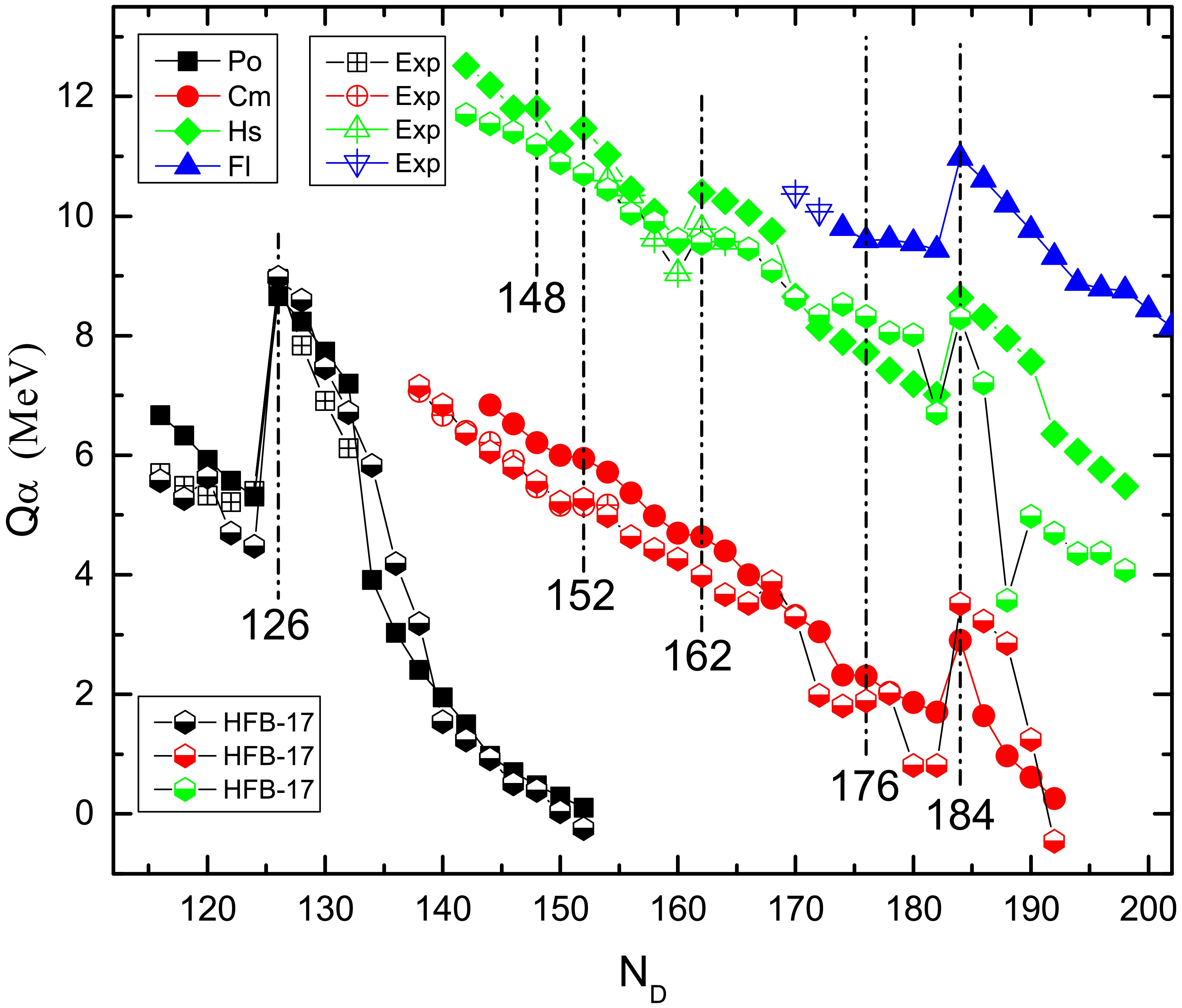

Figure 2.  (color online) Calculated (solid symbols), experimental [76, 77] (open symbols), and HFB-17 [78] (half-open symbols) α-decay Q-values as functions of the daughter neutron number $ N_D $ for even- N isotopes of Po, Cm, Hs, and Fl.

The shell closures could also be indicated from the drop in the values of $ Q_{\alpha} $. A strong drop in $ Q_{\alpha} $ may indicate an increase in the parent stability relative to the adjacent isotopes [30]. This effect appears at $ N_D $ = 134 for Po isotopes and at $ N_D $ =170,192 for Hs isotopes, which indicates that those daughters result from the decay of stable parents, i.e., N = 136 may correspond to sub-shell closures in $ ^{220} $Po, and N = 172 and 194 may correspond to sub-shell closures in $ ^{280} $Hs and $ ^{302} $Hs [9, 50]. The same effect is observed at $ N_D $ =174 in the Cm isotope chain, which indicates the stability of $ ^{272} $Cm. The signature of shell stabilization may appear in the values of $ Q_{\alpha} $ if the parent, and/or the daughter, are shell stabilized.

To assess the predictive performance of our framework, we systematically compared the calculated α-decay Q-values with experimental data and with the self-consistent HFB-17 mass model. The analysis reveals that both approaches demonstrate excellent and complementary agreement with experimental results. A strong global correlation is observed for both models, with coefficients of $ R = 0.971 $ ($ R^2 = 0.943 $) for our calculation and an excellent value of $ R = 0.992 $ ($ R^2 = 0.985 $) for HFB-17. Quantitatively, the root mean square error (RMSE) is $ 0.709 $ MeV for our model, indicating robust predictive capability, while the HFB-17 model achieves an even tighter global accuracy with an RMSE of $ 0.401 $ MeV. The predictive strength of both models is rigorously tested in the superheavy domain. For the Hassium isotopes, the HFB-17 model demonstrates excellent precision, while our model also performs reliably, successfully capturing the systematic trend. Furthermore, both models successfully capture key shell-related features. This is exemplified by their performance on benchmark nuclei adjacent to shell closures: for $ ^{212} $Po, a nucleus whose decay is dominated by the double-magic $ ^{208} $Pb core, our model is within 290 keV of the experimental value, while the HFB-17 prediction is exceptionally precise at 21 keV. Conversely, for the more complex, transitional nucleus $ ^{208} $Po, our model shows improved accuracy, predicting within 355 keV compared to the HFB-17 result within 521 keV. Overall, these results confirm that the HFB-17 model sets a benchmark for numerical accuracy, while our model provides a highly competitive, physically intuitive, and reliable description across the nuclear chart, reproducing structural trends reliably across the chart.

Following the analysis of $ Q_\alpha $ values, Fig. 3 provides further insight into the α-decay process by presenting the penetrability and assault frequency as functions of the daughter neutron number $ N_D $ for even-N isotopes of Po, Cm, Hs, and Fl. These quantities are central to the quantum tunneling aspect of α-decay, and their variations offer a sensitive probe of the underlying nuclear structure, particularly shell effects. The assault frequency reflects the characteristics of the internal potential pocket, where the α-particle is preformed, including its shape, width, and depth. In contrast, the penetrability is governed by the properties of the external potential barrier, which the α-particle must tunnel through to complete the decay process. Consequently, both penetrability and assault frequency demonstrate high sensitivity to variations in nuclear potential at two distinct phases of the α-decay process, covering the full trajectory of the preformed α-particle throughout the decay process. This sensitivity positions them as effective probes for investigating structural changes across isotopic chains.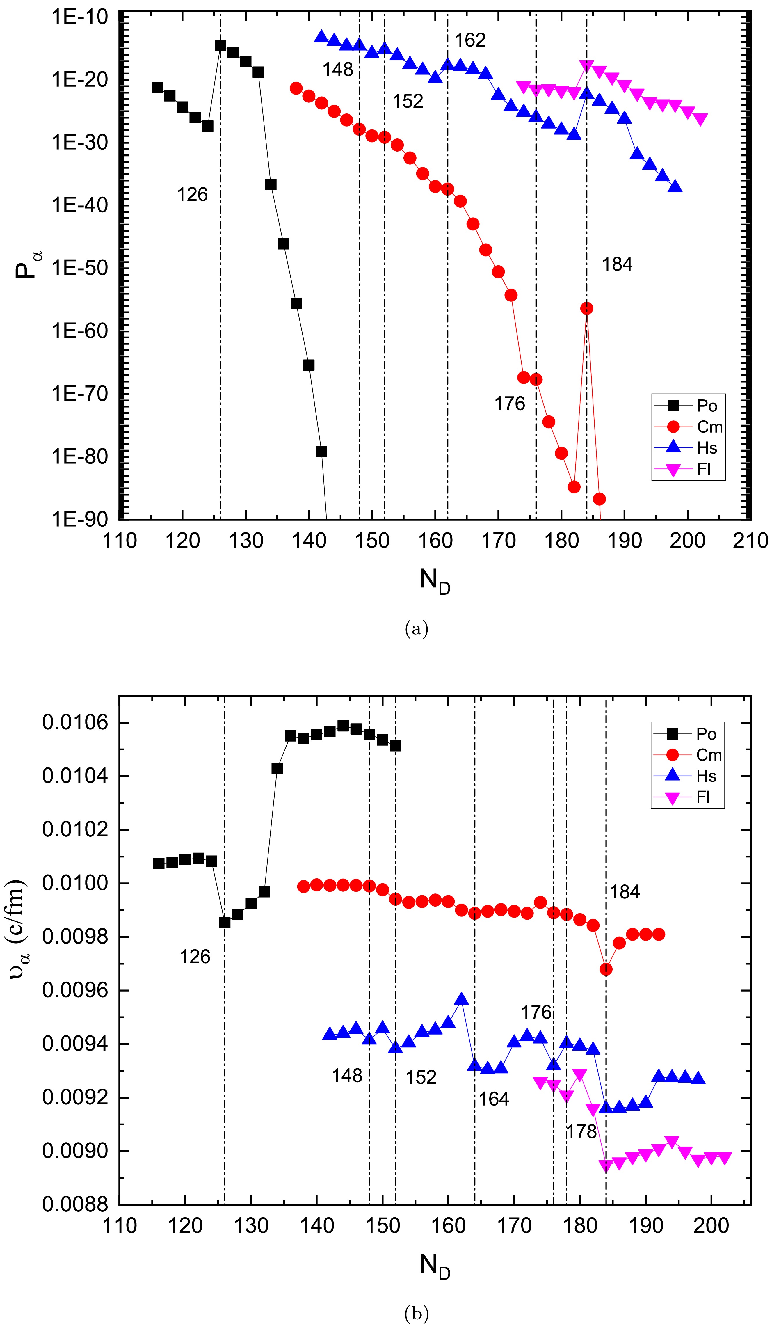

Figure 3.  (color online) (a) Penetrability $ P_\alpha $ and (b) assault frequency $ \nu_\alpha $, plotted as functions of the daughter neutron number $ N_D $ for even- N isotopes of Po, Cm, Hs, and Fl.

In Fig. 3(a), which shows the behavior of penetrability, clear shifts are observed at $ N_D = 126 $ in Po isotopes and at $ N_D = 184 $ in Cm, Hs, and Fl isotopes. These peaks correspond to well-established or theoretically predicted neutron magic numbers. The neutron number $ N = 126 $ marks a classic spherical shell closure, resulting from the complete filling of the $ 1i_{11/2} $ orbital following the $ 3p_{1/2} $, $ 2f_{5/2} $, and $ 3p_{3/2} $ shells. This closure is notably observed in the doubly-magic nucleus $ ^{208} $Pb ($ Z=82 $, $ N=126 $). Meanwhile, $ N = 184 $ is a predicted spherical magic number in the superheavy region, attributed to the filling of the $ 4s_{1/2} $ and $ 2h_{11/2} $ orbitals, beyond the $ 1j_{13/2} $ level. This prediction is supported by both macroscopic-microscopic models such as the finite-range droplet model (FRDM) [8] and self-consistent mean-field calculations [9, 79]. The enhancement in penetrability at these neutron numbers can be attributed to the high binding energy of the resulting daughter nuclei, which reduces the effective potential barrier and increases the decay probability.

Figure 3(b) illustrates the variation in the assault frequency with $ N_D $, where pronounced minima appear at $ N_D = 126 $ and $ N_D = 184 $. In the context of the semi-classical tunneling model, a low assault frequency may be interpreted as a reduction in the depth of the potential well where the α-particle is preformed, expected when the daughter nucleus is particularly stable due to shell closure. The stability of the daughter nucleus creates a more energetically favorable final state for the α-decay process, which reduces the binding of the α-particle in the parent nucleus. This manifests as a shallower potential well for the α-daughter interaction and, consequently, a lower assault frequency. This anti-correlation between penetrability and assault frequency is a hallmark of enhanced nuclear stability and is consistent with findings from cluster formation studies [11, 12], which show that shell closures suppress the preformation factor and shift the decay characteristics.

In addition to these prominent features, secondary anomalies appear at $ N_D = 148 $, 152, and 162, particularly in Cm and Hs isotopes. These neutron numbers are associated with deformed shell gaps predicted in Nilsson-level schemes and deformed mean-field models. The number $ N = 148 $ is linked to partial filling of deformed orbitals derived from spherical subshells near $ 2f_{7/2} $ and $ 3p_{3/2} $. The enhancement at $ N = 152 $ is often associated with a deformed shell gap involving intruder orbitals, such as $ 1i_{13/2} $. Meanwhile, the anomaly at $ N = 162 $ is commonly related to a deformed closure resulting from the alignment of orbitals such as $ 2g_{9/2} $ and $ 1j_{15/2} $ in strongly deformed configurations. These features indicate the presence of shape-stabilized configurations and enhanced binding due to deformation effects. Although the penetrability and assault frequency anomalies at these neutron numbers are less pronounced compared to the spherical magic numbers, their consistency across different isotopic chains supports the existence of local shell effects.

Overall, the systematic shifts in penetrability and assault frequency across neutron numbers reveal both spherical and deformed shell closures. The strong anomalies at $ N = 126 $ and $ N = 184 $ reaffirm their magic character as major shell closures, while the subtler variations at $ N = 148 $, 152, and 162 demonstrate the influence of nuclear deformation and the dependence of shell gaps on both neutron and proton configurations.

Figure 4 shows the values of log($ T_{1/2} $) for α-decays of even- N isotopes $ ^{202-238} $Po, $ ^{236-290} $Cm, $ ^{252-308} $Hs, and $ ^{290-318} $Fl, in that order. The values calculated in the present study are compared to those from 10 other models, namely, Dong, Sobiczewski (Viola Seborg with adjusted parameters) [60], mB1, Groyer, Shree, UDL, NGNF, SLB, Parkhomenko, and Denisov [74, 75]. The lifetimes obtained from most of the methods have almost the same behavior with a change in neutron number. The values calculated in the present study are fully theoretical, either in the calculation of α-daughter potential, estimation of $ Q_{\alpha} $, or calculation of the barrier penetration and lifetime. However, the values obtained in this study and those obtained by other methods, even those based on experimental values, exhibit the same behavior. In addition to the similarity in trends, the values obtained in the present study are within the values obtained by other models.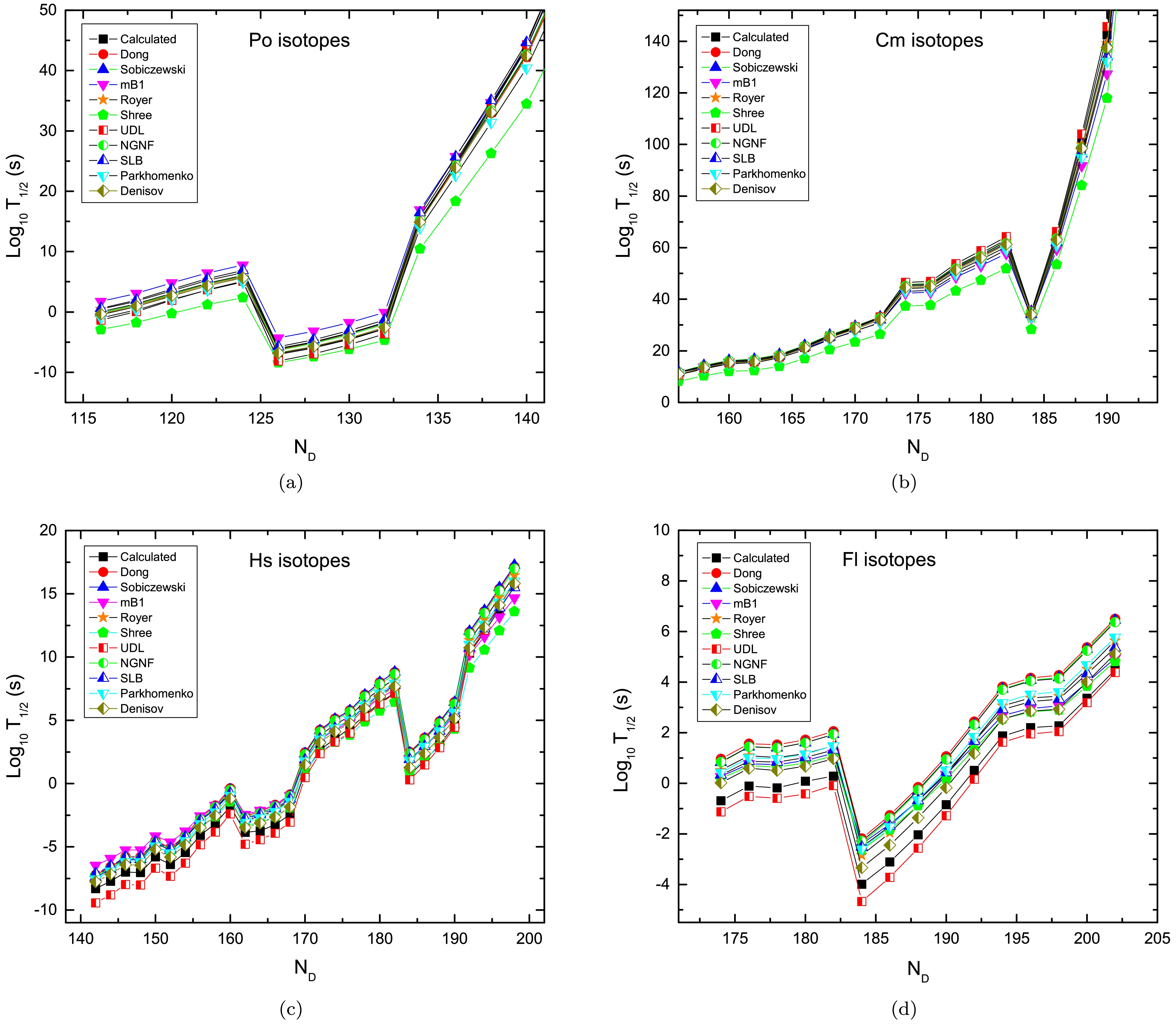

Figure 4.  (color online) Calculated α-decay half-lives plotted as functions of the daughter neutron number, $ N_D $ for (a) Po, (b) Cm, (c) Hs, and (d) Fl isotopes. The values calculated by other models, namely, Dong [32], Sobiczewski (Viola-Seaborg with adjusted parameters) [60], mB1 [33], G Royer [28], Shree [34], UDL [29], NGNF [80], SLB [80], Parkhomenko [30], and Denisov [74, 75], are plotted for comparison.

The general trend shows increasing lifetime with neutron number, reflecting reduced decay energy and increasing nuclear stability against α-decay. For some values of N, the nuclei have extra stabilization because of the shell effect; this effect may cause deviation from the general trend of lifetime change with N if the parent or daughter is shell stabilized. Naturally, nuclei tend to be stabilized, and the lifetime will be relatively low if the daughter is shell stabilized. In contrast, if the parent is shell stabilized, it stays bound for a longer time and the lifetime will be relatively high. For the decay of the Po isotope series, we can observe a drop in the lifetime at $ N_D $ = 126 and an increase at $ N_D $ = 134. This indicates that N = 126 represents a neutron shell closure in the daughter nucleus $ ^{208} $Pb, and N =136 represents a neutron shell closure in the parent nucleus $ ^{220} $Po. For the Cm decay series, there is an obvious drop in lifetime at $ N_D $ = 184, corresponding to neutron shell closure, and a rise at $ N_D $ = 174 corresponding to neutron shell closure at N = 176 in the parent $ ^{272} $Cm.

For Hs isotope decays, there are many points corresponding to significant deviations from the overall trend. We can observe drops at $ N_D $ = 148,152,162, and 184, indicating the possibility of shell or sub-shell closures at those neutron numbers. In fact, the four observed drops differ in strength, but the one observed at $ N_D $ = 184 is the most important for two reasons. First, the drop is clear and strong, and second, the same effect is observed in all isotope chains considered in the present study. This behavior supports the magicity of the neutron number N = 184, as reported in many studies [7−9]. The other drops observed in the Hs chain are less strong than the drop at N = 184 and are not observed in all chains. This indicates that the energy gaps around those neutron numbers are small and depend on the proton number. There are also two significant rises in the lifetime graph of Hs isotopes, particularly at $ N_D $ = 170,192.

The two drops indicate that those daughters result from the decay of relatively stable parents with $ N_p $ = 172 and 194 ($ ^{280} $Hs and $ ^{302} $Hs). For the Fl isotope chain, there is a very important landmark at $ N_D $ =184, which supports the observations from the Cm and Hs chains. There is also a change in the variation trend around $ N_D $ = 194−198, which may be important. In conclusion, the variation in α-decay lifetime by adding successive pairs of neutrons to the parent nucleus is not systematic; some pairs cause notable unsystematic variations because they fill up a shell or sub-shell. In the present study, many values of neutron number are associated with significant changes in α-decay lifetime. The most important changes are observed at N = 126 and 184; the other values listed above are somewhat local and depend on the atomic number Z.

Empirical correlations are crucial in uncovering systematic trends in nuclear decay properties, particularly in regimes where a comprehensive microscopic theory remains elusive. Figure 5 presents the correlation between the logarithm of the α-decay half-life, $ \log_{10}(T_{1/2}) $, and the composite variable $ X = Z^{0.68} Q_{\alpha}^{-1/2} $, which integrates the dominant physical mechanisms: Coulomb repulsion and quantum tunneling. The figure includes both experimental reference data and half-lives calculated from the present microscopic model, providing a direct validation of the proposed scaling framework.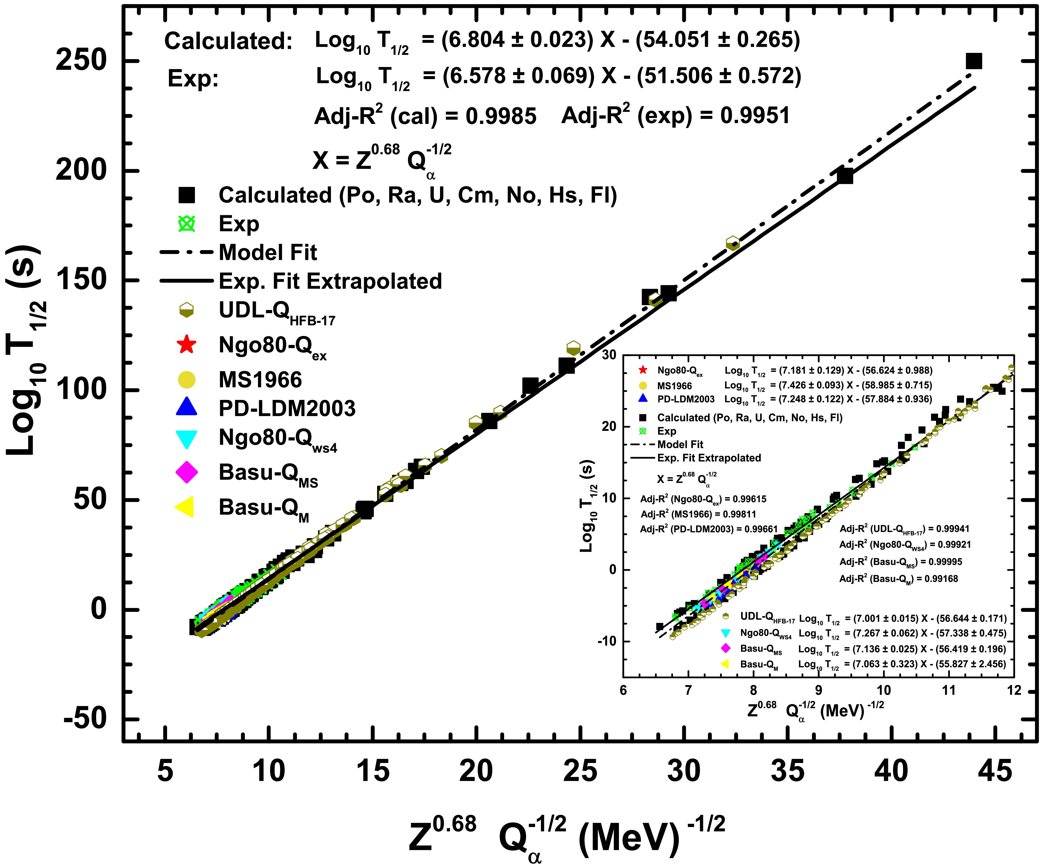

Figure 5.  (color online) Linear correlation between the logarithm of the α-decay half-life, $ \log_{10}(T_{1/2}) $, and the composite variable $ X = Z^{0.68} Q_\alpha^{-1/2} $ for even-even isotopes of Po, Ra, U, Cm, No, Hs, and Fl. The main panel presents both calculated half-lives from the present microscopic model and experimental data [76, 77]. Comparative fits are also shown based on microsccopic HFB-17 calculations [78] in conjunction with the UDL model, proximity potential-based models including Ngo80-$ Q_{\text{ex}} $, Ngo80-$ Q_{\text{WS4}} $, MS1966, PD-LDM2003, and QWS4 [81], and the microscopic WKB-DDM3Y model by Samanta et al. [82], using $ Q_\alpha $ values from the Muntian (M) and Myers-Swiatecki (MS) mass evaluations. The embedded subplot provides a magnified view over the interval $ X \in [6, 12]$.

For the present theoretical model, the best-fit regression yields

with an adjusted coefficient of determination exceeding 0.995, indicating strong linearity across the evaluated isotopes. The corresponding fit to experimental data yields

with a slightly higher $ R^2 \approx 0.9985 $. The proximity of the two regression lines confirms the reliability of the scaling variable X in capturing α-decay systematics, both for predictive modeling and retrospective validation.

To further assess the generality of the proposed framework, Fig. 5 incorporates regression fits from several established models, as indicated in the plot. These include proximity-based approaches, such as Ngo80, using both experimental and calculated WS4 $ Q_\alpha $ values, MS1966, PD-LDM2003, and QWS4 [81], as well as the microscopic WKB-based formalism introduced by Samanta et al. [82]. The Ghodsi-type models employ modified double-folding techniques, utilizing proximity potentials derived from realistic nucleon density distributions and are specifically optimized for α-decay barrier penetration. Conversely, the model of Samanta et al. calculates α-decay half-lives by evaluating quantum mechanical tunneling probabilities through nucleus-nucleus potentials constructed from the DDM3Y density-dependent effective interaction, independent of empirical fitting to decay systematics. These comparative regressions yield slope values typically in the range of 7.1−7.4 and intercepts between $ -55 $ and $ -59 $, with adjusted coefficients of determination consistently exceeding 0.99. The narrow dispersion among these models, despite differences in underlying physical assumptions, further substantiates the robustness and transferability of the composite variable $ X = Z^{0.68} Q_\alpha^{-1/2} $ as a universal scaling descriptor for α-decay systematics.

In addition to the results obtained with experimental $ Q_\alpha $ values, we examined the performance of the correlation with the decay energies taken from the self-consistent Skyrme HFB-17 model table [78] incorporated within the UDL framework. The regression analysis yields an adjusted coefficient of determination $ R^2_{\mathrm{adj}} = 0.99941 $, with

The slope and intercept obtained from the HFB-17-based fit fall well within the narrow range defined by the other models, indicating that the X –scaling is essentially independent of the specific source of $ Q_\alpha $ values. In particular, the close proximity of the HFB-17 regression line to both experimental data and microscopic approaches, such as the WKB–DDM3Y model, as well as to proximity potential systematics, demonstrates that the present correlation captures the dominant structural dependence across different theoretical frameworks. The consistency observed between phenomenological fits and microscopic predictions affirms the structural robustness of the $ X = Z^{0.68} Q_\alpha^{-1/2} $ variable as a unifying descriptor across diverse decay models. The modest spread in slopes (from 6.57 to 7.43) reflects variations in how deformation, pairing, or shell effects are incorporated, yet the overall clustering and strong correlations support the broad applicability of the scaling law. This strongly motivates the continued use of the X -scaling formalism in both retrospective analysis and forward-looking extrapolations into the superheavy region.

This result aligns with the findings of Royer [28], who proposed a relation of the form $ \log_{10}(T_{1/2}) = a Z Q_\alpha^{-1/2} + b $ with coefficients tuned for different nucleon parities. While Royer's formulation uses a linear dependence on Z, the use of $ Z^{0.68} $ in the present study slightly softens the Coulomb effect to better capture trends in superheavy nuclei, as suggested in earlier modifications by Poenaru et al. [31] and Mohr [33]. The current model provides a better fit, particularly in regions where deformation and shell effects might subtly alter decay rates. Moreover, the minimal dispersion in the residuals reflects its strong predictive power.

To quantitatively validate the choice of the exponent $ a = 0.68 $ in the scaling variable $ X = Z^a Q_\alpha^{-1/2} $, a statistical analysis was conducted by plotting the adjusted coefficient of determination $ R^2_{\text{adj}} $ as a function of a. As illustrated in Fig. 6, the resulting curve is well represented by the vertex form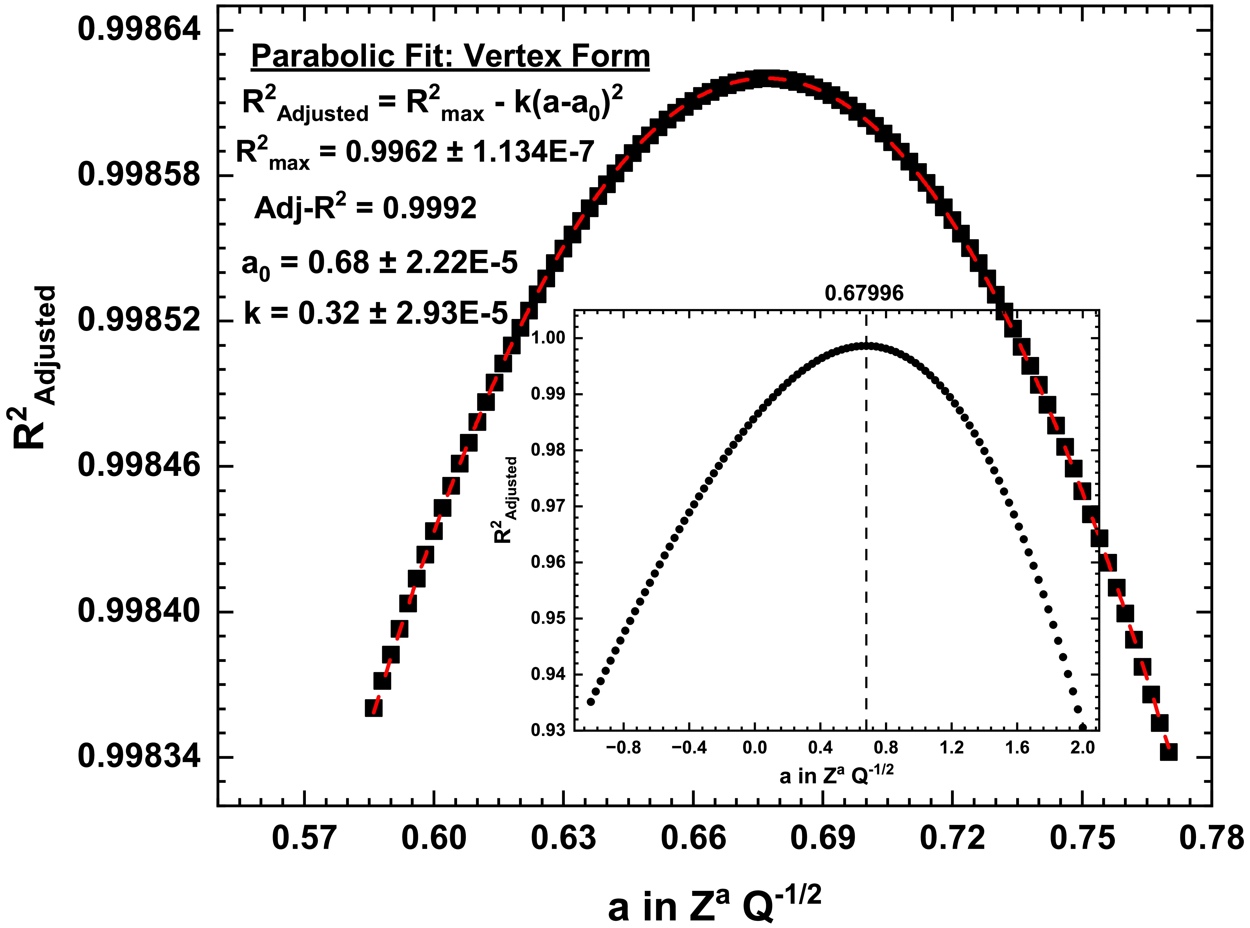

Figure 6.  (color online) Adjusted coefficient of determination $ R^2_{\text{adj}} $ plotted against the scaling exponent a of the composite variable X in the empirical decay correlation. The main curve highlights the region near the optimum fit, while the embedded plot displays the full trend over the broader interval $ a \in [-1, 2] $, confirming the uniqueness and stability of the statistical maximum.

where the best-fit values are $ a_0 = 0.68 \pm 2.2 \times 10^{-5} $, $ k = 0.32 \pm 2.9 \times 10^{-5} $, and $ R^2_{\text{max}} = 0.9962 \pm 1.1 \times 10^{-7} $. This parabolic behavior clearly demonstrates that the maximum statistical agreement is attained at $ a = 0.68 $, validating the empirical exponent used in the composite variable X.

The very narrow uncertainty in the fitted vertex and high goodness of fit (adjusted $ R^2 = 0.9992 $) affirm the uniqueness and robustness of this exponent choice. The sublinear scaling in Z implied by the value $ a = 0.68 $ likely reflects effective nuclear structure effects, including shell and deformation contributions. The relatively sharp curvature encoded by the parameter k further indicates that even minor deviations from the optimal exponent reduce the correlation strength, underscoring the precision and physical soundness of the adopted scaling relation.

To further assess the universality and predictive capacity of the proposed scaling variable, Fig. 7 recasts several well established α-decay models in terms of the composite variable $ X = Z^{0.68} Q_\alpha^{-1/2} $. This unified treatment allows for a direct comparison of linear regression behavior across diverse theoretical and empirical formulations. Each model yields a high adjusted coefficient of determination ($ R^2_{\text{adj}} > 0.999 $), demonstrating that, despite the differences in physical underpinnings, the variable X encapsulates the dominant decay mechanisms with remarkable consistency.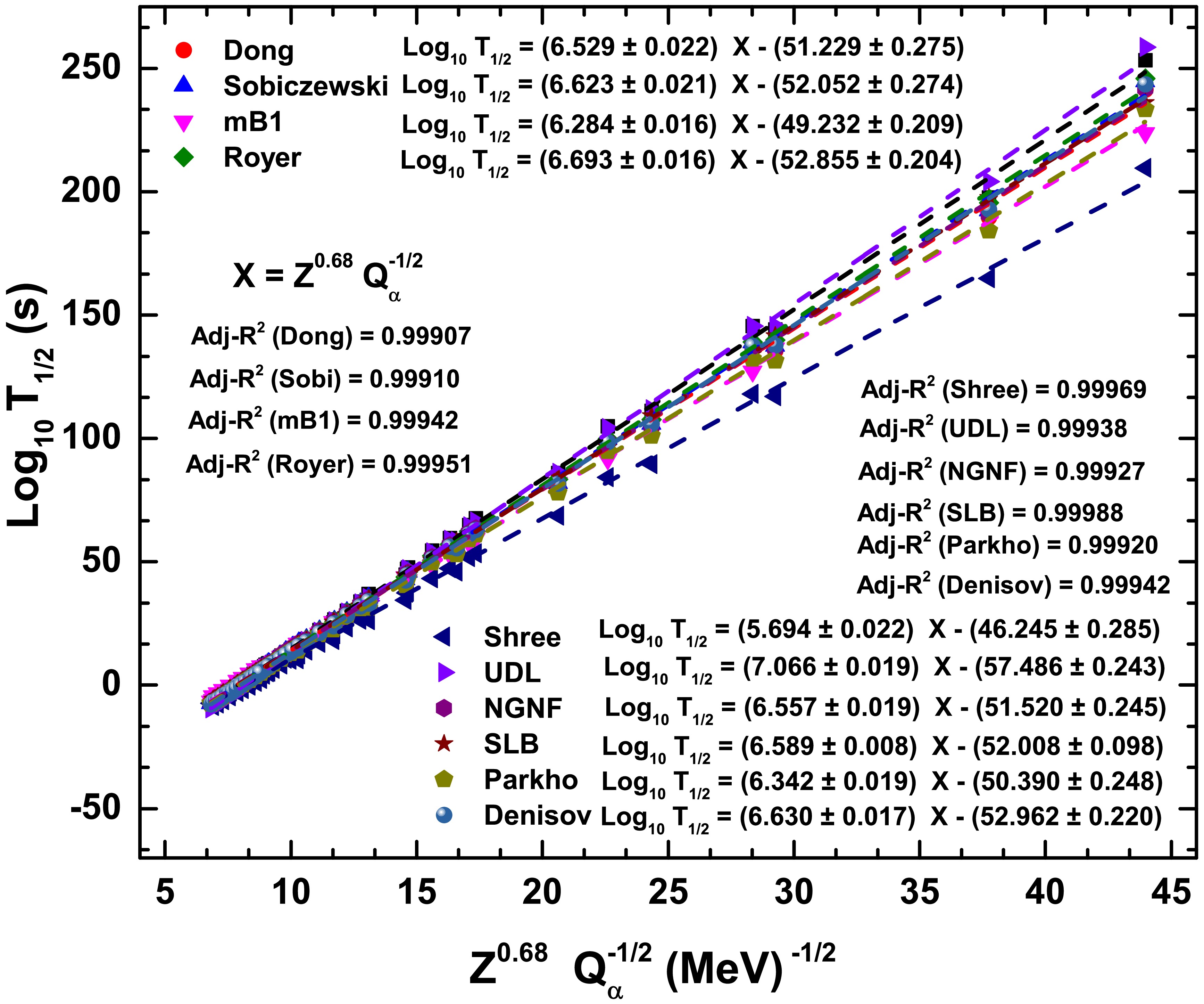

Figure 7.  (color online) Correlation between $ \log(T_{1/2}) $ half-lives and the composite variable X = $ Z^{0.68} Q_\alpha $ for Po, Cm, Hs and Fl isotopes. Global views comparing the current model with several existing ones: Dong [32], Sobiczewski [60], mB1 [33], Royer [28], Shree [34], UDL [29], NGNF [80], SLB [80], Parkhomenko [30], and Denisov [74, 75].

Among the empirical and semi-microscopic models, Royer's formulation [28] produces a fit of

with $ R^2_{\text{adj}} = 0.99951 $, closely paralleling the present model and validating its use across even-even emitters. The Universal Decay Law (UDL) [29] follows with a slightly steeper slope of ($ 7.066 \pm 0.019 $) and an intercept ($ -57.486 \pm 0.243 $), reflecting its broader formulation applicable to both α and cluster decays.

Models incorporating structural corrections such as Denisov-Khudenko [83] and Parkhomenko-Denisov also show high conformity, with slopes of ($ 6.630 \pm 0.017 $) and ($ 6.342 \pm 0.019 $), respectively. Notably, the mB1 model [33] exhibits a slightly lower slope $ (6.284 \pm 0.016) $, indicating a somewhat softer dependence on X, though still achieving $ R^2_{\text{adj}} = 0.99942 $. Among the remaining models, NGNF and SLB [80] display consistent behavior with slopes near 6.55-6.59 and exceptionally high $ R^2 $ values, particularly SLB with $ R^2_{\text{adj}} = 0.99988 $, the highest among all fits. Shree's model [34], while exhibiting the lowest slope $ (5.694 \pm 0.022) $, still maintains excellent statistical agreement.

Taken together, the slopes across all models cluster within the range $ 5.69 \leq m \leq 7.07 $, with intercepts within $ -57.5 \leq b \leq -46.2 $, reflecting modest variation in how individual models encode microscopic corrections such as shell closures, pairing effects, and deformation. Nonetheless, the tight regression clustering in X-space reinforces the conclusion that $ X = Z^{0.68} Q_\alpha^{-1/2} $ effectively captures the leading-order physics of α-decay. This convergence across diverse models, empirical, semi-empirical, and microscopic, strongly supports the adoption of the present scaling variable as a unifying descriptor. Overall, the results affirm that this X -based formalism provides a physically motivated, statistically robust, and broadly applicable framework for systematizing α-decay half-lives across the nuclear chart.

The current model, with its consistently high adjusted $ R^2 $, low dispersion of residuals, and agreement with known systematics, appears well-suited for extrapolation into regions where experimental data are sparse, particularly beyond $ Z = 114 $. This extrapolation reliability is supported by the model's stability across a wide mass range and its ability to reproduce known half-life trends without overfitting. Unlike models that rely on strong parameter tuning or are constrained to narrower domains, the proposed scaling framework maintains predictive accuracy while avoiding abrupt deviations in unmeasured regions. The convergence of multiple models around similar slopes and intercepts when expressed in terms of the proposed variable $ X = Z^{0.68} Q_\alpha^{-1/2} $ further reinforces the generality and physical soundness of the formalism.

Building upon the theoretical approach introduced in Sec. II that integrates the nuclear structure calculations with quantum tunneling theory, we examined the α-decay systematics in even-N isotopic chains of $ ^{202-238} $Po, $ ^{236-290} $Cm, $ ^{252-308} $Hs and $ ^{290-318} $Fl. The analysis focuses on three fundamental aspects: (1) Energy landscapes derived based on Skyrme functionals with dynamical multidimensional optimization procedure, (2) α-daughter interaction potentials constructed from nucleon density distributions, and (3) decay probabilities computed via the WKB approximation. By tracking the evolution of $ Q_\alpha $ values, half-lives, and decay widths across neutron numbers, we identify systematic patterns that reflect underlying nuclear structure effects. These results are compared with available experimental data and established phenomenological models, providing a robust test of the theoretical framework's predictive capability across heavy and superheavy mass regions. The detailed numerical results from these calculations are compiled in Table 2, which provides a comprehensive overview of the α-decay observables for the even-N isotopes of Po, Cm, Hs and Fl. This table includes the calculated $ Q_\alpha $ values (in MeV), renormalization factors λ, assault frequencies $ \nu_\alpha $ (in c/fm), barrier penetrabilities $ P_\alpha $, and logarithmic half-lives $ \log_{10}(T_{1/2}) $ from our approach. For comparative purposes, it also features half-life predictions fromselected phenomenological approaches [29, 33, 74, 75] alongside available experimental $ Q_\alpha $ values and half-lives [76, 77].

Parent	$ Q_\alpha^{\text{calc}} $	$ Q_\alpha^{\text{exp}} $	λ	$ \nu_{\alpha} $	$ P_{\alpha} $	$ {\rm Log}T_{\alpha}^{\text{calc}} $	$ {\rm Log}T_{\alpha}^{\text{mB1}} $	$ {\rm Log}T_{\alpha}^{\text{UDL}} $	$ {\rm Log} T_{\alpha}^{\text{Denisov}} $	$ {\rm Log} T_{\alpha}^{\text{exp}} $
$ ^{202} $Po	6.674	5.701	0.685	0.01007	6.58E-22	0.823	1.754	−1.335	−0.355	5.143
$ ^{204} $Po	6.333	5.485	0.683	0.01008	3.02E-23	2.286	3.073	0.069	0.959	6.277
$ ^{206} $Po	5.923	5.327	0.682	0.01009	5.05E-25	4.156	4.805	1.925	2.699	7.145
$ ^{208} $Po	5.571	5.216	0.680	0.01009	1.04E-26	5.956	6.445	3.681	4.344	7.961
$ ^{210} $Po	5.309	5.408	0.678	0.01008	4.56E-28	7.186	7.770	5.094	5.666	7.078
$ \boxed{^{212} {\text{Po}}}$	8.664	8.954	0.740	0.00985	2.87E-15	−5.717	−4.319	−8.155	−6.811	−6.531
$ ^{214} $Po	8.233	7.834	0.738	0.00988	2.22E-16	−4.702	−3.193	−6.960	−5.693	−3.787
$ ^{216} $Po	7.736	6.906	0.737	0.00992	8.57E-18	−3.363	−1.778	−5.449	−4.278	−0.839
$ ^{218} $Po	7.195	6.115	0.737	0.00997	1.64E-19	−1.700	−0.076	−3.624	−2.567	2.269
$ ^{220} $Po	3.916	−	0.753	0.01043	2.28E-37	16.108	16.922	14.926	14.879	−
$ ^{222} $Po	3.033	−	0.759	0.01055	8.51E-47	25.520	25.747	24.542	23.918	−
$ ^{224} $Po	2.412	−	0.755	0.01054	2.64E-56	35.039	34.688	34.286	33.077	−
$ ^{226} $Po	1.953	−	0.753	0.01055	3.92E-66	44.898	43.874	44.300	42.487	−
$ ^{228} $Po	1.504	−	0.752	0.01057	7.51E-80	58.667	56.674	58.268	55.616	−
$ ^{230} $Po	0.973	−	0.752	0.01059	4.24E-107	85.987	82.103	86.052	81.737	−
$ ^{232} $Po	0.698	−	0.749	0.01058	3.94E-132	111.114	105.564	111.687	105.833	−
$ ^{234} $Po	0.484	−	0.747	0.01056	5.94E-165	144.268	136.540	145.547	137.660	−
$ ^{236} $Po	0.290	−	0.744	0.01054	1.84E-218	197.641	190.105	204.124	192.724	−
$ ^{238} $Po	0.105	−	0.742	0.01051	1.40E-258	237.648	348.273	377.153	355.394	−
$ ^{236} $Cm	7.824	7.067	0.740	0.00999	4.91E-22	0.668	1.324	−0.890	0.138	3.355
$ ^{238} $Cm	7.462	6.670	0.739	0.01	2.62E-23	1.972	2.504	0.453	1.395	5.314
$ ^{240} $Cm	7.167	6.398	0.737	0.00999	2.05E-24	3.130	3.530	1.617	2.483	6.370
$ ^{242} $Cm	6.840	6.216	0.735	0.00999	9.92E-26	4.519	4.742	2.999	3.775	7.148
$ ^{244} $Cm	6.526	5.902	0.734	0.00999	4.27E-27	5.979	5.996	4.429	5.113	8.757
$ ^{246} $Cm	6.216	5.475	0.732	0.00999	1.50E-28	7.764	7.323	5.947	6.533	11.172
$ ^{248} $Cm	5.999	5.162	0.730	0.00998	1.26E-29	8.705	8.313	7.069	7.581	13.079
$ \boxed{^{250} {\text{Cm}}}$	5.946	5.170	0.727	0.00994	7.16E-30	8.838	8.563	7.329	7.819	12.163
$ ^{252} $Cm	5.722	−	0.725	0.00993	4.53E-31	9.943	9.659	8.577	8.985	−
$ ^{254} $Cm	5.366	−	0.723	0.00993	3.74E-33	11.954	11.536	10.738	11.009	−
$ ^{256} $Cm	4.984	−	0.723	0.00994	1.21E-35	14.393	13.769	13.316	13.425	−
$ ^{258} $Cm	4.702	−	0.721	0.00993	1.12E-37	16.395	15.592	15.415	15.391	−
$\boxed{ ^{260} {\text{Cm}}}$	4.642	−	0.718	0.0099	4.13E-38	16.818	16.003	15.864	15.806	−
$ ^{262} $Cm	4.404	−	0.716	0.00989	5.23E-40	18.726	17.703	17.820	17.637	−
$ ^{264} $Cm	4.003	−	0.715	0.0099	1.25E-43	22.378	20.912	21.541	21.126	−
$ ^{266} $Cm	3.611	−	0.715	0.0099	9.45E-48	26.553	24.554	25.769	25.091	−
$ ^{268} $Cm	3.322	−	0.713	0.0099	3.09E-51	30.111	27.631	29.338	28.436	−
$ ^{270} $Cm	3.051	−	0.712	0.00989	5.78E-55	33.933	30.917	33.150	32.010	−
$ ^{272} $Cm	2.326	−	0.713	0.00993	4.52E-68	47.153	42.370	46.518	44.558	−
$\boxed{ ^{274} {\text{Cm}}}$	2.309	−	0.710	0.00989	2.01E-68	47.643	42.707	46.883	44.893	−
$ ^{276} $Cm	2.035	−	0.709	0.00988	3.76E-75	54.527	48.594	53.740	51.325	−
$ ^{278} $Cm	1.863	−	0.707	0.00986	3.79E-80	59.701	52.972	58.834	56.101	−
$ ^{280} $Cm	1.700	−	0.706	0.00984	1.61E-85	64.897	57.678	64.311	61.236	−
$\boxed{ ^{282} {\text{Cm}}}$	2.901	−	0.695	0.00968	4.52E-57	37.050	32.935	35.334	34.018	−
$ ^{284} $Cm	1.646	−	0.699	0.00978	2.04E-87	67.631	59.387	66.255	63.045	−
$ ^{286} $Cm	0.972	−	0.701	0.00981	1.83E-124	104.937	91.730	104.074	98.545	−
$ ^{288} $Cm	0.618	−	0.700	0.00981	6.89E-165	145.643	127.262	145.629	137.549	−
$ ^{290} $Cm	0.257	−	0.700	0.00981	2.28E-272	253.425	223.775	258.552	243.551	−
$ ^{252} $Hs	12.512	−	0.724	0.00943	5.10E-14	−7.174	−6.473	−9.435	−7.765	−
$ ^{254} $Hs	12.188	−	0.723	0.00944	1.33E-14	−6.519	−5.926	−8.795	−7.169	−
$ ^{256} $Hs	11.803	−	0.722	0.00945	2.45E-15	−5.690	−5.247	−7.989	−6.417	−
$\boxed{ ^{258} {\text{Hs}}}$	11.803	−	0.718	0.00942	2.65E-15	−5.452	−5.247	−8.024	−6.456	−
$ ^{260} $Hs	11.213	−	0.719	0.00946	1.57E-16	−4.363	−4.140	−6.689	−5.207	−
$\boxed{ ^{262} {\text{Hs}}}$	11.469	−	0.714	0.00938	6.19E-16	−5.069	−4.631	−7.332	−5.817	−
$ ^{264} $Hs	11.025	−	0.713	0.0094	6.93E-17	−4.213	−3.768	−6.298	−4.852	−
$ ^{266} $Hs	10.445	10.591	0.714	0.00944	3.06E-18	−2.933	−2.559	−4.835	−3.483	−2.796
$ ^{268} $Hs	10.071	10.346	0.713	0.00945	3.63E-19	−2.060	−1.727	−3.839	−2.552	−2.408
$ ^{270} $Hs	9.571	9.760	0.713	0.00948	1.64E-20	−0.746	−0.536	−2.397	−1.204	−0.398
$\boxed{ ^{272} {\text{Hs}}}$	10.393	9.070	0.722	0.00956	1.75E-18	−2.788	−2.448	−4.800	−3.467	1.182
$ ^{274} $Hs	10.250	−	0.703	0.00932	1.35E-18	−2.655	−2.131	−4.442	−3.136	−
$ ^{276} $Hs	10.052	−	0.701	0.00931	4.44E-19	−2.140	−1.682	−3.920	−2.651	−
$ ^{278} $Hs	9.746	−	0.700	0.00931	7.07E-20	−1.290	−0.964	−3.062	−1.851	−
$ ^{280} $Hs	8.651	−	0.703	0.0094	3.34E-23	2.104	1.917	0.475	1.466	−
$ ^{282} $Hs	8.136	−	0.704	0.00943	5.43E-25	3.986	3.469	2.367	3.236	−
$ ^{284} $Hs	7.895	−	0.702	0.00942	7.09E-26	4.985	4.248	3.300	4.107	−
$ ^{286} $Hs	7.724	−	0.695	0.00932	1.08E-26	5.943	4.822	3.978	4.738	−
$ ^{288} $Hs	7.422	−	0.699	0.0094	9.66E-28	7.143	5.885	5.264	5.940	−
$ ^{290} $Hs	7.192	−	0.698	0.00939	1.02E-28	8.299	6.739	6.291	6.899	−
$ ^{292} $Hs	7.011	−	0.696	0.00938	1.63E-29	8.919	7.438	7.126	7.677	−
$\boxed{ ^{294} {\text{Hs}}}$	8.638	−	0.684	0.00916	5.23E-23	2.265	1.955	0.296	1.260	−
$ ^{296} $Hs	8.310	−	0.683	0.00916	4.05E-24	3.241	2.931	1.474	2.360	−
$ ^{298} $Hs	7.955	−	0.682	0.00917	2.11E-25	4.409	4.050	2.830	3.628	−
$ ^{300} $Hs	7.563	−	0.682	0.00918	6.10E-27	5.853	5.382	4.450	5.144	−
$ ^{302} $Hs	6.359	−	0.687	0.00928	1.23E-32	11.472	10.203	10.399	10.721	−
$ ^{304} $Hs	6.059	−	0.686	0.00927	2.65E-34	13.085	11.624	12.131	12.341	−
$ ^{306} $Hs	5.757	−	0.685	0.00927	4.09E-36	14.866	13.165	14.012	14.101	−
$ ^{308} $Hs	5.483	−	0.684	0.00927	6.86E-38	16.631	14.673	15.852	15.823	−
$ ^{290} $Fl	9.800	9.856	0.702	0.00926	1.22E-21	0.473	0.262	−1.130	0.014	1.580
$ ^{292} $Fl	9.595	−	0.700	0.00925	3.23E-22	1.164	0.773	−0.514	0.588	−
$ ^{294} $Fl	9.609	−	0.697	0.00921	3.85E-22	1.226	0.738	−0.591	0.510	−
$ ^{296} $Fl	9.544	−	0.703	0.00929	2.07E-22	1.648	0.902	−0.414	0.671	−
$ ^{298} $Fl	9.435	−	0.693	0.00916	1.31E-22	1.852	1.185	−0.087	0.973	−
$\boxed{ ^{300} {\text{Fl}}}$	10.975	−	0.681	0.00895	2.55E-18	−2.583	−2.389	−4.672	−3.336	−
$ ^{302} $Fl	10.611	−	0.680	0.00896	3.35E-19	−1.837	−1.615	−3.718	−2.446	−
$ ^{304} $Fl	10.196	−	0.680	0.00898	2.82E-20	−0.878	−0.682	−2.562	−1.366	−
$ ^{306} $Fl	9.765	−	0.680	0.00899	1.80E-21	0.221	0.347	−1.283	−0.170	−
$ ^{308} $Fl	9.313	−	0.680	0.00901	8.01E-23	1.500	1.505	0.160	1.179	−
$ ^{310} $Fl	8.885	−	0.683	0.00904	3.40E-24	2.819	2.679	1.625	2.548	−
$ ^{312} $Fl	8.785	−	0.679	0.009	1.63E-24	3.108	2.966	1.959	2.857	−
$ ^{314} $Fl	8.755	−	0.676	0.00897	1.38E-24	3.173	3.056	2.042	2.930	−
$ ^{316} $Fl	8.444	−	0.676	0.00898	1.12E-25	4.272	3.985	3.195	4.006	−
$ ^{318} $Fl	8.141	−	0.675	0.00898	8.44E-27	5.427	4.941	4.382	5.115	−

Table 2.  Calculated α-decay observables for even-N isotopes of Po, Cm, Hs, and Fl. The table lists the parent nucleus along with the calculated and experimental decay energies $ Q_\alpha^{\text{calc}} $ (MeV) and $ Q_\alpha^{\text{exp}} $ (MeV), renormalization factor λ, assault frequency $ \nu_\alpha $ (c/fm), and barrier penetrability $ P_\alpha $. It also includes the logarithm of the calculated half-life $ \log_{10}[T_{1/2}^{\text{calc}}(\text{s})] $, as well as theoretical half-life predictions from different models: $ \log_{10}[T_{1/2}^{\text{mB1}}(\text{s})] $, $ \log_{10}[T_{1/2}^{\text{UDL}}(\text{s})] $, and $ \log_{10}[T_{1/2}^{\text{Denisov}}(\text{s})] $, alongside the available experimental value $ \log_{10}[T_{1/2}^{\text{exp}}(\text{s})] $ for comparison. The boxed nuclei correspond to daughter nuclei with magic or quasi-magic neutron numbers.

Figure 2 shows $ Q_\alpha $ values obtained using the macroscopic-microscopic method for the α-decays of even-N isotopes $ ^{202-238} $Po, $ ^{236-290} $Cm, $ ^{252-308} $Hs, and $ ^{290-318} $Fl. The available empirical data from Refs. [76, 77] for the four isotopic chains are shown on the same graph, showing the matches in trends and behavior, in addition to proximity of values. $ Q_\alpha $ quantifies the difference in binding energy between the parent nucleus and its decay products, serving as a direct indicator of decay energetics. Furthermore, the available results of the self-consistent HFB-17 mass model [78] are also plotted for comparison. Generally, a monotonic decrease in $ Q_\alpha $ with increasing neutron number is observed, consistent with the movement toward the neutron drip line and reduced decay energy. However, there are some values of N corresponding to significant deviations in $ Q_{\alpha} $ from the general trend. Those deviations indicate neutron shell, or sub-shell, closures. The signature of shell closure is clear and strong at $ N_D $ = 126,184; moreover, it is observed in all chains considered in Fig 2. The clear shift in the case of $ N_D $ = 126,184 results from the large values of binding energy of daughters with magic N, as predicted by macroscopic-microscopic models [8, 30], which leads to large values of $ Q_{\alpha} $. The signature of neutron shell or sub-shell closures also appears at $ N_D $ = 148,152,162, and 176, consistent with predictions of deformed shell structure [8, 51]. The deviation differs from the case of $ N_D $ = 126,184 in two characteristics: (1) the deviation is not as strong, and (2) the signature is not present in all isotopes chains. For N = 148, the signature appears in the Hs isotope series only, while for N = 176, the signature barely appears in the Cm isotope series only. For $ N_D $ = 152 and 162, the signature appears in both Cm and Hs isotope chains, but the signature is more clear in the Hs isotope chain. The variation in the strength of the shell closure signature for the same N value may be attributed to the effect of proton number on the neutron shells [11, 36].

Figure 2.  (color online) Calculated (solid symbols), experimental [76, 77] (open symbols), and HFB-17 [78] (half-open symbols) α-decay Q-values as functions of the daughter neutron number $ N_D $ for even- N isotopes of Po, Cm, Hs, and Fl.

The shell closures could also be indicated from the drop in the values of $ Q_{\alpha} $. A strong drop in $ Q_{\alpha} $ may indicate an increase in the parent stability relative to the adjacent isotopes [30]. This effect appears at $ N_D $ = 134 for Po isotopes and at $ N_D $ =170,192 for Hs isotopes, which indicates that those daughters result from the decay of stable parents, i.e., N = 136 may correspond to sub-shell closures in $ ^{220} $Po, and N = 172 and 194 may correspond to sub-shell closures in $ ^{280} $Hs and $ ^{302} $Hs [9, 50]. The same effect is observed at $ N_D $ =174 in the Cm isotope chain, which indicates the stability of $ ^{272} $Cm. The signature of shell stabilization may appear in the values of $ Q_{\alpha} $ if the parent, and/or the daughter, are shell stabilized.

To assess the predictive performance of our framework, we systematically compared the calculated α-decay Q-values with experimental data and with the self-consistent HFB-17 mass model. The analysis reveals that both approaches demonstrate excellent and complementary agreement with experimental results. A strong global correlation is observed for both models, with coefficients of $ R = 0.971 $ ($ R^2 = 0.943 $) for our calculation and an excellent value of $ R = 0.992 $ ($ R^2 = 0.985 $) for HFB-17. Quantitatively, the root mean square error (RMSE) is $ 0.709 $ MeV for our model, indicating robust predictive capability, while the HFB-17 model achieves an even tighter global accuracy with an RMSE of $ 0.401 $ MeV. The predictive strength of both models is rigorously tested in the superheavy domain. For the Hassium isotopes, the HFB-17 model demonstrates excellent precision, while our model also performs reliably, successfully capturing the systematic trend. Furthermore, both models successfully capture key shell-related features. This is exemplified by their performance on benchmark nuclei adjacent to shell closures: for $ ^{212} $Po, a nucleus whose decay is dominated by the double-magic $ ^{208} $Pb core, our model is within 290 keV of the experimental value, while the HFB-17 prediction is exceptionally precise at 21 keV. Conversely, for the more complex, transitional nucleus $ ^{208} $Po, our model shows improved accuracy, predicting within 355 keV compared to the HFB-17 result within 521 keV. Overall, these results confirm that the HFB-17 model sets a benchmark for numerical accuracy, while our model provides a highly competitive, physically intuitive, and reliable description across the nuclear chart, reproducing structural trends reliably across the chart.

Following the analysis of $ Q_\alpha $ values, Fig. 3 provides further insight into the α-decay process by presenting the penetrability and assault frequency as functions of the daughter neutron number $ N_D $ for even-N isotopes of Po, Cm, Hs, and Fl. These quantities are central to the quantum tunneling aspect of α-decay, and their variations offer a sensitive probe of the underlying nuclear structure, particularly shell effects. The assault frequency reflects the characteristics of the internal potential pocket, where the α-particle is preformed, including its shape, width, and depth. In contrast, the penetrability is governed by the properties of the external potential barrier, which the α-particle must tunnel through to complete the decay process. Consequently, both penetrability and assault frequency demonstrate high sensitivity to variations in nuclear potential at two distinct phases of the α-decay process, covering the full trajectory of the preformed α-particle throughout the decay process. This sensitivity positions them as effective probes for investigating structural changes across isotopic chains.

Figure 3.  (color online) (a) Penetrability $ P_\alpha $ and (b) assault frequency $ \nu_\alpha $, plotted as functions of the daughter neutron number $ N_D $ for even- N isotopes of Po, Cm, Hs, and Fl.

In Fig. 3(a), which shows the behavior of penetrability, clear shifts are observed at $ N_D = 126 $ in Po isotopes and at $ N_D = 184 $ in Cm, Hs, and Fl isotopes. These peaks correspond to well-established or theoretically predicted neutron magic numbers. The neutron number $ N = 126 $ marks a classic spherical shell closure, resulting from the complete filling of the $ 1i_{11/2} $ orbital following the $ 3p_{1/2} $, $ 2f_{5/2} $, and $ 3p_{3/2} $ shells. This closure is notably observed in the doubly-magic nucleus $ ^{208} $Pb ($ Z=82 $, $ N=126 $). Meanwhile, $ N = 184 $ is a predicted spherical magic number in the superheavy region, attributed to the filling of the $ 4s_{1/2} $ and $ 2h_{11/2} $ orbitals, beyond the $ 1j_{13/2} $ level. This prediction is supported by both macroscopic-microscopic models such as the finite-range droplet model (FRDM) [8] and self-consistent mean-field calculations [9, 79]. The enhancement in penetrability at these neutron numbers can be attributed to the high binding energy of the resulting daughter nuclei, which reduces the effective potential barrier and increases the decay probability.

Figure 3(b) illustrates the variation in the assault frequency with $ N_D $, where pronounced minima appear at $ N_D = 126 $ and $ N_D = 184 $. In the context of the semi-classical tunneling model, a low assault frequency may be interpreted as a reduction in the depth of the potential well where the α-particle is preformed, expected when the daughter nucleus is particularly stable due to shell closure. The stability of the daughter nucleus creates a more energetically favorable final state for the α-decay process, which reduces the binding of the α-particle in the parent nucleus. This manifests as a shallower potential well for the α-daughter interaction and, consequently, a lower assault frequency. This anti-correlation between penetrability and assault frequency is a hallmark of enhanced nuclear stability and is consistent with findings from cluster formation studies [11, 12], which show that shell closures suppress the preformation factor and shift the decay characteristics.

In addition to these prominent features, secondary anomalies appear at $ N_D = 148 $, 152, and 162, particularly in Cm and Hs isotopes. These neutron numbers are associated with deformed shell gaps predicted in Nilsson-level schemes and deformed mean-field models. The number $ N = 148 $ is linked to partial filling of deformed orbitals derived from spherical subshells near $ 2f_{7/2} $ and $ 3p_{3/2} $. The enhancement at $ N = 152 $ is often associated with a deformed shell gap involving intruder orbitals, such as $ 1i_{13/2} $. Meanwhile, the anomaly at $ N = 162 $ is commonly related to a deformed closure resulting from the alignment of orbitals such as $ 2g_{9/2} $ and $ 1j_{15/2} $ in strongly deformed configurations. These features indicate the presence of shape-stabilized configurations and enhanced binding due to deformation effects. Although the penetrability and assault frequency anomalies at these neutron numbers are less pronounced compared to the spherical magic numbers, their consistency across different isotopic chains supports the existence of local shell effects.

Overall, the systematic shifts in penetrability and assault frequency across neutron numbers reveal both spherical and deformed shell closures. The strong anomalies at $ N = 126 $ and $ N = 184 $ reaffirm their magic character as major shell closures, while the subtler variations at $ N = 148 $, 152, and 162 demonstrate the influence of nuclear deformation and the dependence of shell gaps on both neutron and proton configurations.

Figure 4 shows the values of log($ T_{1/2} $) for α-decays of even- N isotopes $ ^{202-238} $Po, $ ^{236-290} $Cm, $ ^{252-308} $Hs, and $ ^{290-318} $Fl, in that order. The values calculated in the present study are compared to those from 10 other models, namely, Dong, Sobiczewski (Viola Seborg with adjusted parameters) [60], mB1, Groyer, Shree, UDL, NGNF, SLB, Parkhomenko, and Denisov [74, 75]. The lifetimes obtained from most of the methods have almost the same behavior with a change in neutron number. The values calculated in the present study are fully theoretical, either in the calculation of α-daughter potential, estimation of $ Q_{\alpha} $, or calculation of the barrier penetration and lifetime. However, the values obtained in this study and those obtained by other methods, even those based on experimental values, exhibit the same behavior. In addition to the similarity in trends, the values obtained in the present study are within the values obtained by other models.

Figure 4.  (color online) Calculated α-decay half-lives plotted as functions of the daughter neutron number, $ N_D $ for (a) Po, (b) Cm, (c) Hs, and (d) Fl isotopes. The values calculated by other models, namely, Dong [32], Sobiczewski (Viola-Seaborg with adjusted parameters) [60], mB1 [33], G Royer [28], Shree [34], UDL [29], NGNF [80], SLB [80], Parkhomenko [30], and Denisov [74, 75], are plotted for comparison.

The general trend shows increasing lifetime with neutron number, reflecting reduced decay energy and increasing nuclear stability against α-decay. For some values of N, the nuclei have extra stabilization because of the shell effect; this effect may cause deviation from the general trend of lifetime change with N if the parent or daughter is shell stabilized. Naturally, nuclei tend to be stabilized, and the lifetime will be relatively low if the daughter is shell stabilized. In contrast, if the parent is shell stabilized, it stays bound for a longer time and the lifetime will be relatively high. For the decay of the Po isotope series, we can observe a drop in the lifetime at $ N_D $ = 126 and an increase at $ N_D $ = 134. This indicates that N = 126 represents a neutron shell closure in the daughter nucleus $ ^{208} $Pb, and N =136 represents a neutron shell closure in the parent nucleus $ ^{220} $Po. For the Cm decay series, there is an obvious drop in lifetime at $ N_D $ = 184, corresponding to neutron shell closure, and a rise at $ N_D $ = 174 corresponding to neutron shell closure at N = 176 in the parent $ ^{272} $Cm.

For Hs isotope decays, there are many points corresponding to significant deviations from the overall trend. We can observe drops at $ N_D $ = 148,152,162, and 184, indicating the possibility of shell or sub-shell closures at those neutron numbers. In fact, the four observed drops differ in strength, but the one observed at $ N_D $ = 184 is the most important for two reasons. First, the drop is clear and strong, and second, the same effect is observed in all isotope chains considered in the present study. This behavior supports the magicity of the neutron number N = 184, as reported in many studies [7−9]. The other drops observed in the Hs chain are less strong than the drop at N = 184 and are not observed in all chains. This indicates that the energy gaps around those neutron numbers are small and depend on the proton number. There are also two significant rises in the lifetime graph of Hs isotopes, particularly at $ N_D $ = 170,192.

The two drops indicate that those daughters result from the decay of relatively stable parents with $ N_p $ = 172 and 194 ($ ^{280} $Hs and $ ^{302} $Hs). For the Fl isotope chain, there is a very important landmark at $ N_D $ =184, which supports the observations from the Cm and Hs chains. There is also a change in the variation trend around $ N_D $ = 194−198, which may be important. In conclusion, the variation in α-decay lifetime by adding successive pairs of neutrons to the parent nucleus is not systematic; some pairs cause notable unsystematic variations because they fill up a shell or sub-shell. In the present study, many values of neutron number are associated with significant changes in α-decay lifetime. The most important changes are observed at N = 126 and 184; the other values listed above are somewhat local and depend on the atomic number Z.

Empirical correlations are crucial in uncovering systematic trends in nuclear decay properties, particularly in regimes where a comprehensive microscopic theory remains elusive. Figure 5 presents the correlation between the logarithm of the α-decay half-life, $ \log_{10}(T_{1/2}) $, and the composite variable $ X = Z^{0.68} Q_{\alpha}^{-1/2} $, which integrates the dominant physical mechanisms: Coulomb repulsion and quantum tunneling. The figure includes both experimental reference data and half-lives calculated from the present microscopic model, providing a direct validation of the proposed scaling framework.

Figure 5.  (color online) Linear correlation between the logarithm of the α-decay half-life, $ \log_{10}(T_{1/2}) $, and the composite variable $ X = Z^{0.68} Q_\alpha^{-1/2} $ for even-even isotopes of Po, Ra, U, Cm, No, Hs, and Fl. The main panel presents both calculated half-lives from the present microscopic model and experimental data [76, 77]. Comparative fits are also shown based on microsccopic HFB-17 calculations [78] in conjunction with the UDL model, proximity potential-based models including Ngo80-$ Q_{\text{ex}} $, Ngo80-$ Q_{\text{WS4}} $, MS1966, PD-LDM2003, and QWS4 [81], and the microscopic WKB-DDM3Y model by Samanta et al. [82], using $ Q_\alpha $ values from the Muntian (M) and Myers-Swiatecki (MS) mass evaluations. The embedded subplot provides a magnified view over the interval $ X \in [6, 12]$.

For the present theoretical model, the best-fit regression yields

with an adjusted coefficient of determination exceeding 0.995, indicating strong linearity across the evaluated isotopes. The corresponding fit to experimental data yields

with a slightly higher $ R^2 \approx 0.9985 $. The proximity of the two regression lines confirms the reliability of the scaling variable X in capturing α-decay systematics, both for predictive modeling and retrospective validation.

To further assess the generality of the proposed framework, Fig. 5 incorporates regression fits from several established models, as indicated in the plot. These include proximity-based approaches, such as Ngo80, using both experimental and calculated WS4 $ Q_\alpha $ values, MS1966, PD-LDM2003, and QWS4 [81], as well as the microscopic WKB-based formalism introduced by Samanta et al. [82]. The Ghodsi-type models employ modified double-folding techniques, utilizing proximity potentials derived from realistic nucleon density distributions and are specifically optimized for α-decay barrier penetration. Conversely, the model of Samanta et al. calculates α-decay half-lives by evaluating quantum mechanical tunneling probabilities through nucleus-nucleus potentials constructed from the DDM3Y density-dependent effective interaction, independent of empirical fitting to decay systematics. These comparative regressions yield slope values typically in the range of 7.1−7.4 and intercepts between $ -55 $ and $ -59 $, with adjusted coefficients of determination consistently exceeding 0.99. The narrow dispersion among these models, despite differences in underlying physical assumptions, further substantiates the robustness and transferability of the composite variable $ X = Z^{0.68} Q_\alpha^{-1/2} $ as a universal scaling descriptor for α-decay systematics.

In addition to the results obtained with experimental $ Q_\alpha $ values, we examined the performance of the correlation with the decay energies taken from the self-consistent Skyrme HFB-17 model table [78] incorporated within the UDL framework. The regression analysis yields an adjusted coefficient of determination $ R^2_{\mathrm{adj}} = 0.99941 $, with

The slope and intercept obtained from the HFB-17-based fit fall well within the narrow range defined by the other models, indicating that the X –scaling is essentially independent of the specific source of $ Q_\alpha $ values. In particular, the close proximity of the HFB-17 regression line to both experimental data and microscopic approaches, such as the WKB–DDM3Y model, as well as to proximity potential systematics, demonstrates that the present correlation captures the dominant structural dependence across different theoretical frameworks. The consistency observed between phenomenological fits and microscopic predictions affirms the structural robustness of the $ X = Z^{0.68} Q_\alpha^{-1/2} $ variable as a unifying descriptor across diverse decay models. The modest spread in slopes (from 6.57 to 7.43) reflects variations in how deformation, pairing, or shell effects are incorporated, yet the overall clustering and strong correlations support the broad applicability of the scaling law. This strongly motivates the continued use of the X -scaling formalism in both retrospective analysis and forward-looking extrapolations into the superheavy region.

This result aligns with the findings of Royer [28], who proposed a relation of the form $ \log_{10}(T_{1/2}) = a Z Q_\alpha^{-1/2} + b $ with coefficients tuned for different nucleon parities. While Royer's formulation uses a linear dependence on Z, the use of $ Z^{0.68} $ in the present study slightly softens the Coulomb effect to better capture trends in superheavy nuclei, as suggested in earlier modifications by Poenaru et al. [31] and Mohr [33]. The current model provides a better fit, particularly in regions where deformation and shell effects might subtly alter decay rates. Moreover, the minimal dispersion in the residuals reflects its strong predictive power.

To quantitatively validate the choice of the exponent $ a = 0.68 $ in the scaling variable $ X = Z^a Q_\alpha^{-1/2} $, a statistical analysis was conducted by plotting the adjusted coefficient of determination $ R^2_{\text{adj}} $ as a function of a. As illustrated in Fig. 6, the resulting curve is well represented by the vertex form

Figure 6.  (color online) Adjusted coefficient of determination $ R^2_{\text{adj}} $ plotted against the scaling exponent a of the composite variable X in the empirical decay correlation. The main curve highlights the region near the optimum fit, while the embedded plot displays the full trend over the broader interval $ a \in [-1, 2] $, confirming the uniqueness and stability of the statistical maximum.

where the best-fit values are $ a_0 = 0.68 \pm 2.2 \times 10^{-5} $, $ k = 0.32 \pm 2.9 \times 10^{-5} $, and $ R^2_{\text{max}} = 0.9962 \pm 1.1 \times 10^{-7} $. This parabolic behavior clearly demonstrates that the maximum statistical agreement is attained at $ a = 0.68 $, validating the empirical exponent used in the composite variable X.

The very narrow uncertainty in the fitted vertex and high goodness of fit (adjusted $ R^2 = 0.9992 $) affirm the uniqueness and robustness of this exponent choice. The sublinear scaling in Z implied by the value $ a = 0.68 $ likely reflects effective nuclear structure effects, including shell and deformation contributions. The relatively sharp curvature encoded by the parameter k further indicates that even minor deviations from the optimal exponent reduce the correlation strength, underscoring the precision and physical soundness of the adopted scaling relation.

To further assess the universality and predictive capacity of the proposed scaling variable, Fig. 7 recasts several well established α-decay models in terms of the composite variable $ X = Z^{0.68} Q_\alpha^{-1/2} $. This unified treatment allows for a direct comparison of linear regression behavior across diverse theoretical and empirical formulations. Each model yields a high adjusted coefficient of determination ($ R^2_{\text{adj}} > 0.999 $), demonstrating that, despite the differences in physical underpinnings, the variable X encapsulates the dominant decay mechanisms with remarkable consistency.