


 Abstract
 HTML
HTML Reference
 Related
 PDF
PDF


-
Electroweak precision observables have provided a precise test of the standard model (SM) at the loop level [1, 2], which is consistent with the observations of a 125 GeV SM-like Higgs [3, 4]. However, the SM could not provide satisfactory solutions to dark matter, neutrino mass, baryogenesis, etc. [5−8]. Furthermore, the naturalness problem in the SM points to new physics beyond the SM [9].
One of the simplest extensions of the SM Higgs sector is the two-Higgs doublet model (2HDM) [10], which has been studied extensively. The 2HDM can be further extended by an additional singlet field, which is the N2HDM with a real singlet [11−13], and the 2HDM+S with a complex singlet [14, 15]. The 2HDM+S matches the next-to minimal supersymmetric standard model (NMSSM) [16] at a low energy scale and can provide a dark matter candidate [17−19], as well as accommodate the possible 95 GeV excess at the LEP and LHC [15]. The phenomenological properties of the 2HDM+S have only been explored in some specific scenarios, whereas the more general cases of the 2HDM+S have not yet been studied in detail. In this study, we explore the implications of the electroweak precision measurements on the 2HDM+S parameter space. In particular, we focus on the oblique parameters S, T, and U, which are sensitive to the new physics contributions to the W and Z self-energies [20, 21].
The scalar sector of the 2HDM+S includes two
${S U(2)}_L$ doublets and a complex singlet. The singlet field does not couple to the SM gauge bosons and fermions. After the neutral components achieve vacuum expectation values (vev), assuming no CP-violation, the mass spectrum of the Higgs sectors includes 3 CP-even scalars, two CP-odd scalars, and a pair of charged Higgses. In particular, the CP-even and CP-odd singlet components mix with the corresponding ones in the${S U(2)}_L$ doublets, which leads to the couplings of the singlet-like scalars to the SM gauge bosons, as well as modifications of the couplings of the doublet-like scalars to the SM sector. The most general 2HDM+S Higgs potential has 27 free parameters, and 11 of these can be chosen to be the masses of the Higgs bosons, as well as the mixing angles between Higgses. The remaining parameters in the Higgs potential are the Higgs self-couplings, which do not directly contribute to the oblique parameters. Therefore, in our study, we only focus on the STU constraint and the relevant parameters, including these 11 mass and mixing parameters. We parameterize such mixing parameters by$ \alpha_{hS} $ , the mixing of the CP-even singlet with the 125 GeV SM-like Higgs h,$ \alpha_{HS} $ , the mixing of the CP-even singlet with the 2HDM CP-even Higgs H, and$ \alpha_{AS} $ , the mixing of the CP-odd singlet with the 2HDM CP-odd Higgs A.While the general formalism for the contributions of various Higgses to the oblique parameter exists in literature [22], the analyses of electroweak precision constraints in the 2HDM+S could be complex given the enlarged parameter space. In our analyses, we performed a systematic study of the impacts of each mixing angle on the oblique parameters. Including the usual 2HDM mixing angle of the CP-even Higgses α, we introduce five basic benchmark scenarios, Case-0 for the 2HDM alignment limit and Cases-I−IV in which only one mixing angle is set to be nonzero. We analyze the contributions to the oblique parameters in each case and study the 95% C.L. allowed region in the relevant parameter spaces under the oblique parameters. After the discussion of these five benchmark scenarios, we discuss the cases with a non-zero singlet mixing angle away from the alignment limit.
The implications of electroweak precision measurements in the 2HDM and singlet extended SM have been studied in the literature [22−27]. Our study offers a comprehensive electroweak precision analysis of the 2HDM+S and identifies the impact of each singlet mixing angle. As only the couplings between the Higgses and the SM gauge bosons enter the oblique parameters, our results are universal to the 2HDM+S models, with or without further symmetry assumption of the Higgs potential. In addition, we explore the complementarity of the electroweak precision analyses with the Higgs precision measurements. Note that, if we start from the parameters in the Higgs potential for a specific 2HDM+S model, and impose the theoretical considerations of successful electroweak symmetry breaking, vacuum stability, perturbativity, and unitarity, the resulting values of the mixing angles and mass differences might be restricted to a certain range. These ranges would depend on the particular symmetry assumption of the Higgs potential, and could also be relaxed with the variation of other model parameters. In our analyses, we consider a model independent approach and use the various mixing angles and physics Higgs masses as our relevant model parameters for the STU study. We let the mixing angles vary over the whole range and the mass difference up to approximately 1 TeV, which allows a straightforward mapping of a particular Higgs potential scenario to the general results of the electroweak precision constraints that we studied herein.
The remainder of this paper is organized as follows. In Section II, we introduce the theoretical framework of the 2HDM+S, as well as five benchmark cases. In Section III, we introduce the electroweak oblique parameters and the contributions from the Higgs sector in the 2HDM+S. In Section IV, we present 95% C.L. STU allowed regions in the 2HDM+S parameter spaces of the five benchmark cases. In Section V, we study the cases beyond the alignment limit. In Section VI, we show the complementarity of electroweak precision analyses with Higgs precision measurements. We conclude this paper in Section VII.
-
The 2HDM+S is the singlet extension of the 2HDM, which has the following scalar contents:
$ \begin{aligned} \Phi_1=\begin{pmatrix} \chi_1^+\\ \dfrac{{\rho_1+{\rm i}\eta_1}}{\sqrt{2}} \end{pmatrix},\;\;\Phi_2=\begin{pmatrix} \chi_2^+\\ \dfrac{{\rho_2+{\rm i}\eta_2}}{\sqrt{2}} \end{pmatrix},\;\; S= \dfrac{\rho_S + {\rm i}\eta_S}{\sqrt{2}}, \end{aligned} $
(1) where
$ \Phi_1 $ and$ \Phi_2 $ are the SU(2)L doublets with hypercharge$ Y=1/2 $ , and S is the gauge singlet. The general Higgs potential of the 2HDM+S has been introduced in [14], whereas the simplified version of the 2HDM+S potential can be found in [15] when certain symmetries are imposed. After electroweak symmetry breaking, the neutral components of$ \Phi_1 $ ,$ \Phi_2 $ , and S develop non-zero vacuum expectation values,$ v_1 $ ,$ v_2 $ , and$ v_S $ , with$ \sqrt{v_1^2 + v_2^2} = v\approx 246 $ GeV. We also introduce$ \tan\beta = \dfrac{v_2}{v_1} $ with$ \beta \in (0, \pi/2) $ . Assuming no CP-violation, the mass spectrum of the 2HDM+S includes three neutral CP-even scalars, two neutral CP-odd scalars, and one pair of charged Higgs bosons.The neutral CP-even states,
$ \rho_{1,2,S} $ mix together to form three mass eigenstates: the non-SM-like H, the SM-like Higgs h, and the singlet-like$ h_S $ , with the$ 3\times3 $ rotation matrix R$ \begin{aligned} \begin{pmatrix} H\\ h\\ h_S \end{pmatrix} = R \begin{pmatrix} \rho_1\\ \rho_2\\ \rho_S \end{pmatrix},\;\; R M_S^2 R^T = \operatorname{diag}\{m_H^2, m_{h}^2, m_{h_S}^2\}. \end{aligned} $
(2) The R matrix is parameterized using three mixing angles α,
$ \alpha_{HS} $ , and$ \alpha_{hS} $ , which characterize the mixing angle between the two neutral components of the Higgs doublets$ \rho_{1,2} $ , and the mixing angles between the singlet$ \rho_S $ with the 2HDM CP-even Higgses:$ \begin{split} R&= \begin{pmatrix} 1& 0& 0\\ 0& c_{\alpha_{hS}}& s_{\alpha_{hS}}\\ 0& -s_{\alpha_{hS}}& c_{\alpha_{hS}}\\ \end{pmatrix}\begin{pmatrix} c_{\alpha_{HS}}& 0& s_{\alpha_{HS}}\\ 0& 1& 0\\ -s_{\alpha_{HS}}& 0& c_{\alpha_{HS}}\\ \end{pmatrix} \begin{pmatrix} c_{\alpha_{}}& s_{\alpha_{}}& 0\\ -s_{\alpha_{}}& c_{\alpha_{}}& 0\\ 0& 0& 1 \end{pmatrix}\\ &=\begin{pmatrix} c_{\alpha_{}}c_{\alpha_{HS}}& s_{\alpha_{}}c_{\alpha_{HS}}& s_{\alpha_{HS}}\\ -s_{\alpha_{}}c_{\alpha_{hS}}-c_{\alpha_{}}s_{\alpha_{HS}}s_{\alpha_{hS}}& c_{\alpha_{}}c_{\alpha_{hS}}-s_{\alpha_{}}s_{\alpha_{HS}}s_{\alpha_{hS}}& c_{\alpha_{HS}}s_{\alpha_{hS}}\\ s_{\alpha_{}}s_{\alpha_{hS}}-c_{\alpha_{}}s_{\alpha_{HS}}c_{\alpha_{hS}}& -s_{\alpha_{}}s_{\alpha_{HS}}c_{\alpha_{hS}}-c_{\alpha_{}}{{s_{\alpha_{hS}}}}& c_{\alpha_{HS}}c_{\alpha_{hS}} \end{pmatrix}, \end{split} $
(3) where we use the shorthand notations
$ s_{x} = \sin x $ and$ c_{x} = \cos x $ . For the CP-odd states, we have$ \begin{split} \begin{pmatrix} G^0\\ A \\ A_S \end{pmatrix}=\;& \begin{pmatrix}\begin{align} & \begin{matrix} \;1 & 0 & 0 \\ \end{matrix} \\ & \begin{matrix} \begin{matrix} 0 \\ 0 \\ \end{matrix} & R^A \\ \end{matrix} \\ \end{align}\end{pmatrix} \begin{pmatrix} c_{\beta}& s_{\beta}& 0\\ -s_{\beta}& c_{\beta}& 0\\ 0 & 0& 1 \end{pmatrix}\begin{pmatrix} \eta_1 \\ \eta_2 \\ \eta_S \end{pmatrix},\\ R^A = & \begin{pmatrix} c_{\alpha_{AS}}& s_{\alpha_{AS}}\\ -s_{\alpha_{AS}}& c_{\alpha_{AS}} \end{pmatrix}, \\[-1pt]\end{split} $
(4) where
$ G^0 $ is the neutral Goldstone boson, and the angle$ \alpha_{AS} $ is the mixing between the 2HDM pseudoscalar and the singlet pseudoscalar$ \eta_S $ . In addition, the charged sector of the 2HDM+S is the same as that of the 2HDM, containing one pair of charged Higgses$ H^\pm $ and the Goldstone bosons$ G^\pm $ . Each of the mixing angles$ \alpha,\alpha_{HS}, \alpha_{hS},\alpha_{AS} $ varies in the range of$ \begin{aligned} -\frac{\pi}{2}<\alpha_{i}<\frac{\pi}{2}. \end{aligned} $
(5) When
$ \alpha_i = \pm {\pi}/{4} $ , the mixing between the two Higgs bosons reaches maximum, and the properties of the two corresponding scalars flip when$ {\pi}/{4}<|\alpha_i|< {\pi}/{2} $ . Note that the effects of different signs of the mixing angles appear only when all four mixing angles are nonzero. When at least one mixing angle is nonzero, the properties of the Higgs bosons are independent of the sign of the mixing angles. When the theoretical considerations of successful electroweak symmetry breaking, vacuum stability, perturbativity, and unitarity are imposed on the Higgs potential, the resulting values of the mixing angles might be restricted to a smaller range. These ranges would depend on the particular symmetry assumption of the Higgs potential. We consider the whole range of these mixing angles, which allows a straightforward mapping of a particular Higgs potential scenario to the general results of the electroweak precision constraints that we investigate in this study.After the diagonalization of the Higgs mass matrices, there are 11 free parameters for the mass eigenstates: six Higgs boson masses,
$ \tan\beta $ , and four mixing angles. As only the couplings between the Higgses and the SM gauge bosons enter the oblique parameters, we focus on the following nine free parameters for our study of the oblique parameters:$ \begin{aligned} \underbrace{m_h=125\ {\rm{GeV}}, \; m_H,\; m_{A},\; m_{H^\pm},\; \cos(\beta-\alpha),}_{{\rm{2HDM \;parameters}}}\; \underbrace{m_{h_S},\; m_{A_S},\; \alpha_{HS},\; \alpha_{hS},\; \alpha_{AS}}_{{\rm{singlet\; parameters}}}. \end{aligned} $
(6) Using the mixing matrices, one can obtain the couplings of physical Higgses to the gauge bosons, which are denoted by the following effective couplings:
$ \begin{aligned} g_{h_i VV}^{\mu\nu} = c_{h_i VV} {\rm i} \frac{2m_V^2}{v}g^{\mu\nu}, \end{aligned} $
(7) where
$ h_i $ represents all possible neutral CP-even states, including h, H, and$ h_S $ , and$ V=W,\,Z $ . The normalized couplings$ c_{h_i VV} $ are shown in Table 2.Couplings Case-0 Case-I Case-II Case-III Case-IV $ c_{h_i VV}= R_{i1} c_\beta + R_{i2}s_\beta $ $ c_{HVV} $ $ c_{\beta-\alpha}c_{\alpha_{HS}} $ 0 $ c_{\beta-\alpha} $ 0 0 0 $ c_{hVV} $ $ s_{\beta-{\alpha}}c_{\alpha_{hS}} - c_{\beta-{\alpha}}s_{\alpha_{HS}}s_{\alpha_{hS}} $ 1 $ s_{\beta-\alpha} $ $ c_{\alpha_{hS}} $ 1 1 $ c_{h_SVV} $ $ -s_{\beta-\alpha}s_{\alpha_{hS}} - c_{\beta-\alpha}s_{\alpha_{HS}}c_{\alpha_{hS}} $ 0 0 $ -s_{\alpha_{hS}} $ 0 0 $ c_{a_i h_j Z} = R^A_{i1}R_{j1} + R^A_{i2}R_{j2} $ $ c_{A H Z} $ $ -c_{\alpha_{AS}}c_{\alpha_{HS}}s_{\beta-{\alpha}} $ −1 $ -s_{\beta-{\alpha}} $ −1 $ -c_{\alpha_{HS}} $ $ -c_{\alpha_{AS}} $ $ c_{AhZ} $ $ c_{\alpha_{AS}}\Big(c_{\beta-{\alpha}}c_{\alpha_{hS}} + s_{\beta-{\alpha}}s_{\alpha_{HS}}s_{\alpha_{hS}} \Big) $ 0 $ c_{\beta-{\alpha}} $ 0 0 0 $ c_{Ah_S Z} $ $ -c_{\alpha_{AS}}\Big(c_{\beta-{\alpha}}s_{\alpha_{hS}} - s_{\beta-{\alpha}}s_{\alpha_{HS}}c_{\alpha_{hS}} \Big) $ 0 0 0 $ s_{\alpha_{HS}} $ 0 $ c_{A_S HZ} $ $ s_{\alpha_{AS}}c_{\alpha_{HS}}s_{\beta-{\alpha}} $ 0 0 0 0 $ s_{\alpha_{AS}} $ $ c_{A_S h Z} $ $ -s_{\alpha_{AS}}\Big(c_{\beta-{\alpha}}c_{\alpha_{hS}} + s_{\beta-{\alpha}}s_{\alpha_{HS}}s_{\alpha_{hS}} \Big) $ 0 0 0 0 0 $ c_{A_S h_S Z} $ $ s_{\alpha_{AS}}\Big(c_{\beta-{\alpha}}s_{\alpha_{hS}} - s_{\beta-{\alpha}}s_{\alpha_{HS}}c_{\alpha_{hS}} \Big) $ 0 0 0 0 0 $ c_{\phi_i H^\pm W^\mp}=R^{\phi}_{i2}c_\beta - R^{\phi}_{i1}s_\beta $ $ c_{H H^\pm W^\mp} $ $-{\rm i} c_{\alpha_{HS} }s_{\beta-{\alpha} }$ −i $-{\rm i}s_{\beta-{\alpha} }$ −i $-{\rm i}c_{\alpha_{HS} }$ −i $ c_{h H^\pm W^\mp} $ ${\rm i}\Big(c_{\beta-{\alpha} } c_{\alpha_{hS} } + s_{\beta-{\alpha} }s_{\alpha_{HS} }s_{\alpha_{hS} } \Big)$ 0 ${\rm i}c_{\beta-{\alpha} }$ 0 0 0 $ c_{h_S H^\pm W^\mp} $ $-{\rm i}\Big(c_{\beta-{\alpha} } s_{\alpha_{hS} } - s_{\beta-{\alpha} }s_{\alpha_{HS} }c_{\alpha_{hS} } \Big)$ 0 0 0 $-{\rm i}s_{\alpha_{HS} }$ 0 $ c_{A H^\pm W^\mp} $ $ c_{\alpha_{AS}} $ 1 1 1 1 $ c_{\alpha_{AS}} $ $ c_{A_S H^\pm W^\mp} $ $ -s_{\alpha_{AS}} $ 0 0 0 0 $ -s_{\alpha_{AS}} $ $ c_{\phi_i \phi_j VV}=R^{\phi}_{i1}R^{\phi}_{j1}+R^{\phi}_{i2}R^{\phi}_{j2} $ $ c_{HH VV} $ $ c^2_{\alpha_{HS}} $ 1 1 1 $ c^2_{\alpha_{HS}} $ 1 $ c_{h h VV} $ $ c^2_{\alpha_{hS}}+s^2_{\alpha_{HS}} s^2_{\alpha_{hS}} $ 1 1 $ c^2_{\alpha_{hS}} $ 1 1 $ c_{h_S h_S VV} $ $ c^2_{\alpha_{hS}}s^2_{\alpha_{HS}}+ s^2_{\alpha_{hS}} $ 0 0 $ s^2_{\alpha_{hS}} $ $ s^2_{\alpha_{HS}} $ 0 $ c_{H h VV} $ $ -\dfrac{1}{2} s_{2\alpha_{HS}}s_{\alpha_{hS}} $ 0 0 0 0 0 $ c_{H h_S VV} $ $ -\dfrac{1}{2} s_{2\alpha_{HS}}c_{\alpha_{hS}} $ 0 0 0 $ -\dfrac{1}{2}s_{2\alpha_{HS}} $ 0 $ c_{h h_S VV} $ $ -\dfrac{1}{2} c^2_{\alpha_{HS}}s_{2\alpha_{hS}} $ 0 0 $ -\dfrac{1}{2}s_{2\alpha_{hS}} $ 0 0 $ c_{A A VV} $ $ c^2_{\alpha_{AS}} $ 1 1 1 1 $ c^2_{\alpha_{AS}} $ $ c_{A_S A_S VV} $ $ s^2_{\alpha_{AS}} $ 0 0 0 0 $ s^2_{\alpha_{AS}} $ $ c_{A A_S VV} $ $ -\dfrac{1}{2} s_{2\alpha_{AS}} $ 0 0 0 0 $ -\dfrac{1}{2} s_{2\alpha_{AS}} $ $ c_{H^\pm H^\mp Z} $ 1 1 1 1 1 $ c_{H^\pm H^{\mp} \gamma} $ 1 1 1 1 1 $ c_{H^\pm H^\mp VV} $ 1 1 1 1 1 Relevant mixing — $ H,h $ $ h, h_S $ $ H, h_S $ $ A, A_S $ Table 2. Couplings between Higgs bosons and gauge bosons in the 2HDM+S.
In addition, the gauge boson can couple to two different Higgs bosons: the Z boson couples to two Higgs bosons with different CP properties, and the W bosons couple to neutral and charged Higgs bosons. These interactions can be parameterized as
$ \begin{aligned} g^\mu_{\phi_i \varphi_j V} &= c_{\phi_i \varphi_j V} \,{\rm i} \frac{m_V}{v}(p^\mu_{\phi_i}-p^\mu_{\varphi_j}), \end{aligned} $
(8) $ \begin{aligned} g^\mu_{H^- H^+ \gamma} &= c_{H^+ H^- \gamma} \,{\rm i}e (p^\mu_{H^-}-p^\mu_{H^+}), \end{aligned} $
(9) $ \begin{aligned} g^\mu_{H^- H^+ Z} &= c_{H^+ H^- Z} \,{\rm i}e\frac{c_W^2 - s_W^2}{s_W c_W} (p^\mu_{H^-}-p^\mu_{H^+}), \end{aligned} $
(10) where
$ \phi_i $ and$ \varphi_j $ correspond to different types of Higgs bosons: φ includes neutral states, and ϕ includes charged Higgs$ H^\pm $ 1 . Furthermore, the Higgs bosons can couple to gauge bosons via the quartic interactions, which are$ \begin{aligned} {g_{\varphi_i \varphi_j VV}^{\mu\nu}} = c_{\varphi_i \varphi_j VV}\, \frac{{\rm i}2 m_V^2}{v^2} g^{\mu\nu}. \end{aligned} $
(11) Given the complexity of the 2HDM+S scalar sectors and the appearance of multiple mixing angles, we consider five benchmark cases to disentangle the impact of each mixing angle. For Case-0, we have all the mixing angles set to be 0, which is the 2HDM alignment limit case. For other cases, only one mixing angle is nonzero, whereas the others are fixed to 0, as shown in Table 1.
Benchmark Case Fixed mixing angles Variable
mixing anglesCase-0 (2HDM
alignment limit)$ c_{\beta-\alpha}=\alpha_{HS}=\alpha_{hS}=\alpha_{AS}=0 $ — Case-I (2HDM limit) $ \alpha_{HS}=\alpha_{hS}=\alpha_{AS}=0 $ $ c_{\beta-\alpha} $ Case-II (SSM limit) $ c_{\beta-\alpha}=\alpha_{HS}=\alpha_{AS}=0 $ $ \alpha_{hS} $ Case-III $ c_{\beta-\alpha}=\alpha_{hS}=\alpha_{AS}=0 $ $ \alpha_{HS} $ Case-IV $ c_{\beta-\alpha}=\alpha_{hS}=\alpha_{HS}=0 $ $ \alpha_{AS} $ Table 1. Five benchmark cases for the mixing angle configurations
● Case-0 with
$ c_{\beta-\alpha}=\alpha_{HS}=\alpha_{hS}=\alpha_{AS}=0 $ is the 2HDM alignment limit, where the singlet components are decoupled, and the 125 GeV Higgs h is the same as the SM Higgs. In this case, all the couplings of the singlet Higgs bosons$ h_S $ ,$ A_S $ to SM particles are zero, and the beyond the SM (BSM) Higgs coupling HVV is zero. However, the BSM Higgs bosons can still couple to gauge bosons via AHZ,$ H H^\pm W^\mp $ ,$ A H^\pm W^\mp $ , HHVV, AAVV, and$ H^+H^-VV $ couplings.● Case-I with
$ \alpha_{HS}=\alpha_{hS}=\alpha_{AS}=0 $ is the 2HDM limit, when the singlet components are completely decoupled. The mixing between H and h is parameterized by α, as in the usual 2HDM.● Case-II with
$ \alpha_{hS} \neq 0 $ represents the case when the 125 GeV h mixes with the singlet Higgs$ h_S $ ; thus, the SM-like Higgs properties are similar to those of the singlet extended SM (SSM). However, the BSM doublet components$ H/A $ are the same as the alignment limit of the 2HDM.● Case-III with
$ \alpha_{HS} \neq 0 $ represents the case when the non-SM H mixes with the singlet Higgs$ h_S $ , whereas the 125 GeV Higgs h is completely SM-like.● Case-IV with
$ \alpha_{AS} \neq 0 $ represents the case when A mixes with the singlet pseudoscalar$ A_S $ , where the CP-even sector is the same as the alignment limit of the 2HDM, plus a decoupled singlet scalar S.In Table 2, we list the couplings between the Higgses and the SM gauge bosons, which are relevant for the calculation of the oblique parameters. The general expressions are given in the second column, as well as the couplings in the individual Case-0 − Case-IV. As the STU parameters only depend on couplings between the Higgses and gauge bosons, the fermionic couplings of the Higgs bosons are irrelevant in this study. Therefore, the contributions to the STU parameters are independent of the specific structure of the Yukawa couplings. In particular, when the singlet CP-odd Higgs is decoupled by
$ \alpha_{AS}=0 $ , the 2HDM+S is similar to the N2HDM (the real singlet extension of the 2HDM [11]). Note that the$ A_S h Z $ and$ A_S h_S Z $ couplings are always zero for these benchmark cases, as multiple non-zero mixing angles are needed to couple the CP-odd singlet Higgs$ A_S $ to the CP-even Higgs h and$ h_S $ . In addition, the quartic coupling$ HhVV $ is zero for the benchmark cases and is non-zero only when$ \alpha_{HS} $ and$ \alpha_{hS} $ are both non-zero. -
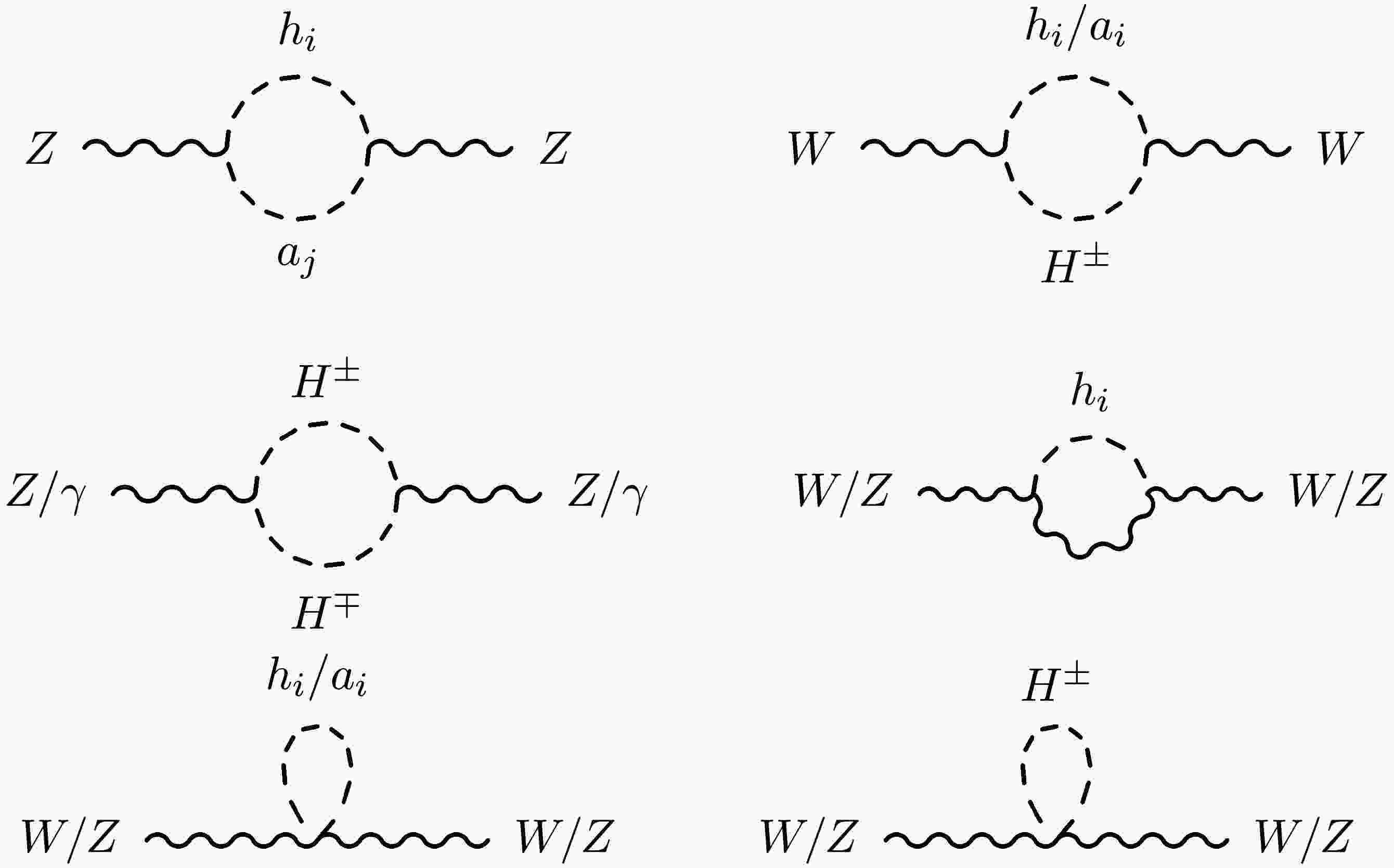
As the oblique parameters STU are constructed with the W and Z self-energies [21], as shown in Eqs. (A2)− (A3), they receive contributions from the Feynman diagrams in Fig. 1. The three-point vertices (including
$ h_i VV $ ,$ h_ia_j Z $ ,$ h_i/a_i H^\pm W^\mp $ , and$ Z/\gamma H^\pm H^\mp $ ), as well as the four-point vertices (including$ h_i h_i VV $ ,$ a_i a_i VV $ , and$ H^\pm H^\mp VV $ ), contribute to the self-energies of the gauge bosons.
Figure 1. Feynman diagrams that contribute to the self energy of the SM gauge bosons.
The contributions to the STU parameters from various Higgses can be found in Ref. [22]. Using those expressions, the STU parameters in the 2HDM+S are given by
$ \begin{split} S=\;&\frac{1}{24\pi}\Bigg[ (2s_W^2-1)^2G(m_{H^\pm}^2,m_{H^\pm}^2,m_Z^2)+\sum_{i,j} |{c_{a_i h_j Z}}|^2 G(m_{a_i}^2,m_{h_j}^2,m_Z^2) +\sum_{i=1}^3 {c_{h_ih_iVV}} \ln(m_{h_i}^2) \\ &+\sum_{i=1}^2 {c_{a_i a_iVV}} \ln(m_{a_i}^2)-2\ln(m_{H^\pm}^2) -\ln(m_{h_{\rm{ref}}}^2) +\sum_{i=1}^3 |c_{h_i VV}|^2 \hat G(m_{h_i}^2,m_Z^2)-\hat G(m_{h_{\rm{ref}}}^2,m_Z^2) \Bigg], \end{split} $
(12) $ \begin{split} T=\;&\frac{1}{16\pi s_W^2 m_W^2}\Bigg[ \sum_{i=1}^3 {|c_{h_i H^\pm W^\mp}|^2} F(m_{H^\pm}^2,m_{h_i}^2)+\sum_{i=1}^2 {|c_{a_i H^\pm W^\mp}|^2}F(m_{H^\pm}^2,m_{a_i}^2) - \sum_{i,j} {|c_{a_i h_j Z}|^2} F(m_{a_i}^2,m_{h_j}^2) \\ &+3 \sum_{i=1}^3 |c_{h_i VV}|^2 \left(F(m_Z^2,m_{h_i}^2)-F(m_W^2,m_{h_i}^2) \right) -3 \left(F(m_Z^2,m_{h_{\rm{ref}}}^2)-F(m_W^2,m_{h_{\rm{ref}}}^2) \right) \Bigg], \end{split} $
(13) $ \begin{split} U=\;&\frac{1}{24\pi}\Bigg[ \sum_{i=1}^3 {|c_{h_i H^\pm W^\mp}|^2}G(m_{H^\pm}^2,m_{h_i}^2,m_W^2)+ \sum_{i=1}^2 {|c_{a_i H^\pm W^\mp}|^2}G(m_{H^\pm}^2,m_{a_i}^2,m_W^2)-(2s_W^2-1)^2 G(m_{H^\pm}^2,m_{H^\pm}^2,m_Z^2)\\ &-\sum_{i,j} {|c_{a_i h_j Z}|}^2 G(m_{a_i}^2,m_{h_j}^2,m_Z^2) +\sum_{i=1}^3 |c_{h_i VV}|^2\left(\hat G(m_{h_i}^2,m_W^2)-\hat G(m_{h_i}^2,m_Z^2) \right)-\hat G(m_{h_{\rm{ref}}}^2,m_W^2)+\hat G(m_{h_{\rm{ref}}}^2,m_Z^2) \Bigg], \end{split} $
(14) where
$ m_{h_{\rm{ref}}}=125 $ GeV is the reference mass of the SM Higgs. The functions F, G, and$ \hat{G} $ can be found in Eqs. (A4), (A5), and (A6) in Appendix A.For the T parameter, the contributions from the quartic couplings are canceled out, as
$ \varphi_i\varphi_i W W $ are the same as$ \varphi_i\varphi_i ZZ $ and the T observable is defined by the self-energy difference between the W boson and Z boson (see Eq. (A1)). Thus, the T observable only receives the contribution from the$ h_i VV $ ,$ a_i h_j Z $ , and$ a_i/h_i H^\pm W^\mp $ couplings. Furthermore, the S parameter mainly represents the Z boson self-energy, and receives contributions from the$ ZH^\pm H^\mp $ interaction via$ G(m_{H^\pm}^2,m_{H^\pm}^2,m_Z^2) $ and the$ a_i h_j Z $ interaction via$ G(m_{a_i}^2,m_{h_j}^2,m_Z^2) $ . In addition, the quartic couplings$ h_i h_i VV $ ,$ a_i a_i VV $ , and$ H^\pm H^\pm VV $ enter into the S parameter via the logarithmic functions. For the U parameter, the contributions of the quartic interactions are canceled out again. Furthermore, the U parameter is related to the dim-8 operator, which is usually suppressed. Therefore, in our discussion below, we mostly focus on the S and T parameters, which are more sensitive to the BSM effects.The experimental measurements for the electroweak precision observables yield the following best-fit values of STU [28] for
$ m_{h_{\rm{ref}}}=125 $ GeV:$ \begin{aligned} \begin{matrix} S^{\rm{exp}}=-0.04, & T^{\rm{exp}}=0.01,& U^{\rm{exp}}=-0.01,\\ \Delta S=0.10, & \Delta T=0.12,& \Delta U=0.09,\\ {\rm{corr}}(S,T)=+0.93, & {\rm{corr}}(S,U)=-0.70,& {\rm{corr}}(T,U)=-0.87, \end{matrix} \end{aligned} $
(15) where
$ {\rm{corr}}(S,T) $ ,$ {\rm{corr}}(S,U) $ , and$ {\rm{corr}}(T,U) $ are the correlation coefficients between S, T, and U. The contributions to the oblique parameters STU in the 2HDM+S, i.e., Eqs. (13), (12), and (14), can be used to obtain the$ \chi^2 $ value [26, 29],$ \begin{aligned} \chi^2_{STU}=\begin{pmatrix} S-S^{\rm{exp}}, & T-T^{\rm{exp}}, & U-U^{\rm{exp}} \end{pmatrix} \cdot {cov}^{-1} \cdot \begin{pmatrix} S-S^{\rm{exp}} \\ T-T^{\rm{exp}} \\ U-U^{\rm{exp}} \end{pmatrix}, \end{aligned} $
(16) where
$ \begin{aligned} {cov}=\begin{pmatrix} \Delta {S}^2 & {\rm{corr}}(S,T) \Delta S\Delta T &{\rm{corr}}(S,U) \Delta S\Delta U\\ {\rm{corr}}(S,T) \Delta S\Delta T & \Delta {T}^2 &{\rm{corr}}(T,U) \Delta T\Delta U\\ {\rm{corr}}(S,U) \Delta S\Delta U & {\rm{corr}}(T,U)\Delta {T}\Delta {U} &\Delta U^2 \end{pmatrix}. \end{aligned} $
(17) The two-dimensional fit to the STU parameters at 95% C.L. corresponds to
$ \Delta\chi^2 = \chi^2_{STU} - \chi^2_{STU}|_{{\rm{minimal}}} < 5.99 $ . -
In the 2HDM, the STU parameters play an important role in constraining the mass splittings between the BSM neutral Higgses and the charged Higgses
$ H^\pm $ . In the 2HDM+S, the singlet field enters via the mixing, which further changes the dependence of the STU parameters on the model parameters. In this section, we explore the impacts of electroweak constraints on the mixing angles,$ \beta-\alpha $ ,$ \alpha_{hS} $ ,$ \alpha_{HS} $ , and$ \alpha_{AS} $ , as well as various mass splittings. For convenience, we define the following mass splittings, which are relevant for the STU constraints:$ \begin{split} &\Delta m_{H} = m_H - m_{H^\pm}, \ \ \ \Delta m_A = m_A - m_{H^\pm},\\ &\Delta m_{h_S}= m_{h_S} - m_{H^\pm}, \ \ \ \Delta m_{A_S} = m_{A_S} - m_{H^\pm}. \end{split} $
(18) With a general scan of the model parameters in the Higgs potential with theoretical considerations taken into account, we find that a relatively large range of mass differences is allowed, particularly with the variation of the soft
$ Z_2 $ breaking mass parameter in the Higgs potential. -
For a starting point, we study the simplest Case-0 (the 2HDM alignment limit) with
$ c_{\beta-\alpha}=\alpha_{HS}=\alpha_{hS}=\alpha_{AS}=0 $ . According to Table 2, the non-zero couplings in this case are$\begin{split} & c_{hVV},\; c_{AHZ},\; c_{HH^\pm W^\mp},\; c_{A H^\pm W^\mp},\; c_{ZH^\pm H^\mp},\\ &c_{hhVV},\; c_{HHVV},\; c_{AAVV},\; c_{H^\pm H^\pm VV}, \end{split}$
(19) with norm 1. The 125 GeV Higgs h is the SM Higgs, and singlet Higgs bosons
$ h_S $ and$ A_S $ both decouple. The doublet BSM Higgses H, A, and$ H^\pm $ enter via AHZ,$ H H^\pm W^\mp $ , and$ A H^\pm W^\mp $ interactions and mainly contribute to the terms involving F functions in the T parameter. In addition,$ Z H^\pm H^\mp $ and quartic interactions HHVV, AAVV, and$ H^\pm H^\mp VV $ contribute to the S parameter. Consequently, the masses of H, A, and$ H^\pm $ are relevant for the oblique parameters, whereas the singlet Higgs masses$ m_{h_S} $ and$ m_{A_S} $ are irrelevant.The T and S parameters in this case, denoted as
$ T_0 $ and$ S_0 $ , respectively, are given by [29]$ T_0 = \frac{1}{16\pi s^2_W m_W^2}[F(m_{H^\pm}^2, m_H^2) - F(m_{A}^2, m_H^2) + F(m_{H^\pm}^2, m_A^2)], $
(20) $ \begin{split} S_0 =\;& \frac{1}{24\pi}[(2s_W^2-1)^2G(m_{H^\pm}^2,m_{H^\pm}^2,m_Z^2) + G(m_A^2, m_H^2, m_Z^2) \\ &+ \ln \left( \frac{m_H^2}{m_{H^\pm}^2} \right) + \ln \left( \frac{m_A^2}{m_{H^\pm}^2} \right) ], \end{split} $
(21) The values of
$ T_0 $ with varying$ \Delta m_H $ and$ \Delta m_A $ are presented by the solid lines in Fig. 2. The left panel indicates varying$ \Delta m_H $ with fixed$ \Delta m_A=0,\ \pm50 $ GeV, and the right panel indicates varying$ \Delta m_A $ with fixed$ \Delta m_H= 0, \pm50 $ GeV. As indicated by Eq. (20),$ T_0 $ is exactly zero when$ \Delta m_H=0 $ or$ \Delta m_A=0 $ . The grey hatch area is the 1σ region of the electroweak precision observable fit to the T parameter.$ T_0 $ is also symmetric under the exchange of$ m_H $ and$ m_A $ . Therefore, the$ T_0 $ dependence on$ \Delta m_H $ in the left panel is the same as the$ T_0 $ dependence on$ \Delta m_A $ in the right panel.$ T_0 $ increases as$ \Delta m_H $ ($ \Delta m_A $ ) increases for$ \Delta m_A>0 $ ($ \Delta m_H >0 $ ) but decreases for the opposite sign of$ \Delta m_A $ ($ \Delta m_H $ ). Furthermore,$ T_0>0 $ when both$ \Delta m_H $ and$ \Delta m_A $ have the same sign, and$ T_0<0 $ when$ \Delta m_H $ and$ \Delta m_A $ have opposite signs.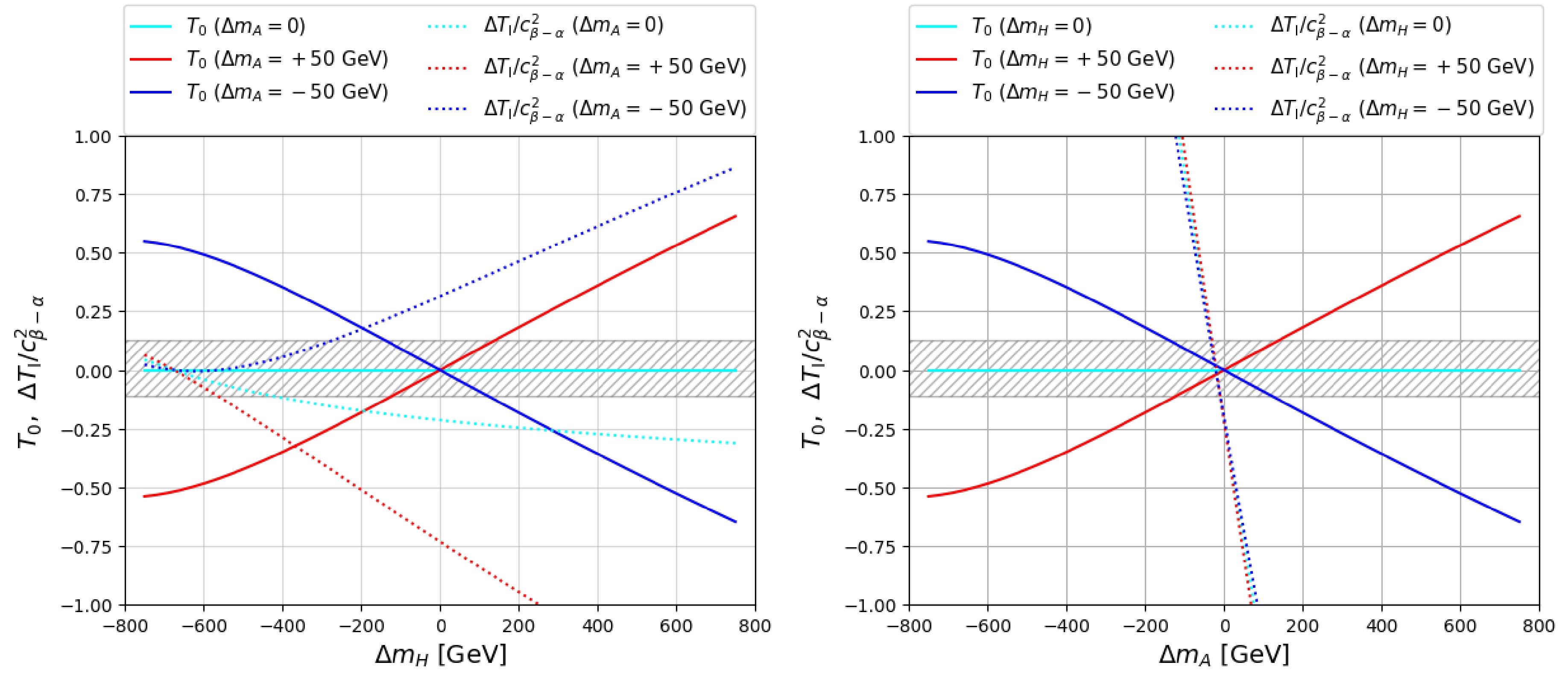
Figure 2. (color online)
$ T_0 $ (solid lines) and$ \Delta T_{\rm{I}}/c^2_{\beta-\alpha} $ (dotted lines) with varying$ \Delta m_H $ (left) and$ \Delta m_A $ (right). The cyan, red, and blue lines indicate$ \Delta m_{A,H}= $ 0, + 50 GeV, and −50 GeV, respectively. The grey hatch area is the 1σ region of the T observable.$ m_{H^\pm} $ is chosen to be 800 GeV.However, the
$ S_0 $ parameter is not zero even when both$ \Delta m_A $ and$ \Delta m_H $ are zero. The contributions from$ G(m_i^2, m_j^2, m_k^2) $ are typically very small. The main contributions to$ S_0 $ come from the logarithmic terms$ \ln(m_{H,A}^2/ m_{H^\pm}^2) $ . For$ \Delta m_{H,A} $ in the range of$ \pm 700 $ GeV,$ |S_0|<0.15 $ is within the 1 σ range of the fitted value.Figure 3 shows the 95% C.L. allowed region from the STU constraints in the
$ \Delta m_H $ vs.$ \Delta m_A $ plane. The blue region corresponds to Case-0 with$ c_{\beta-\alpha}=\alpha_{HS}= \alpha_{hS}= \alpha_{AS}=0 $ and$ m_{H^\pm} = 800 $ GeV, which centers around$ \Delta m_H=0 $ or$ \Delta m_A=0 $ . Owing to the positive correlation between the S and T observables, the area with positive T is preferred. Therefore, the allowed regions with the same signs of$ \Delta m_A $ and$ \Delta m_H $ are larger than the allowed regions with opposite signs.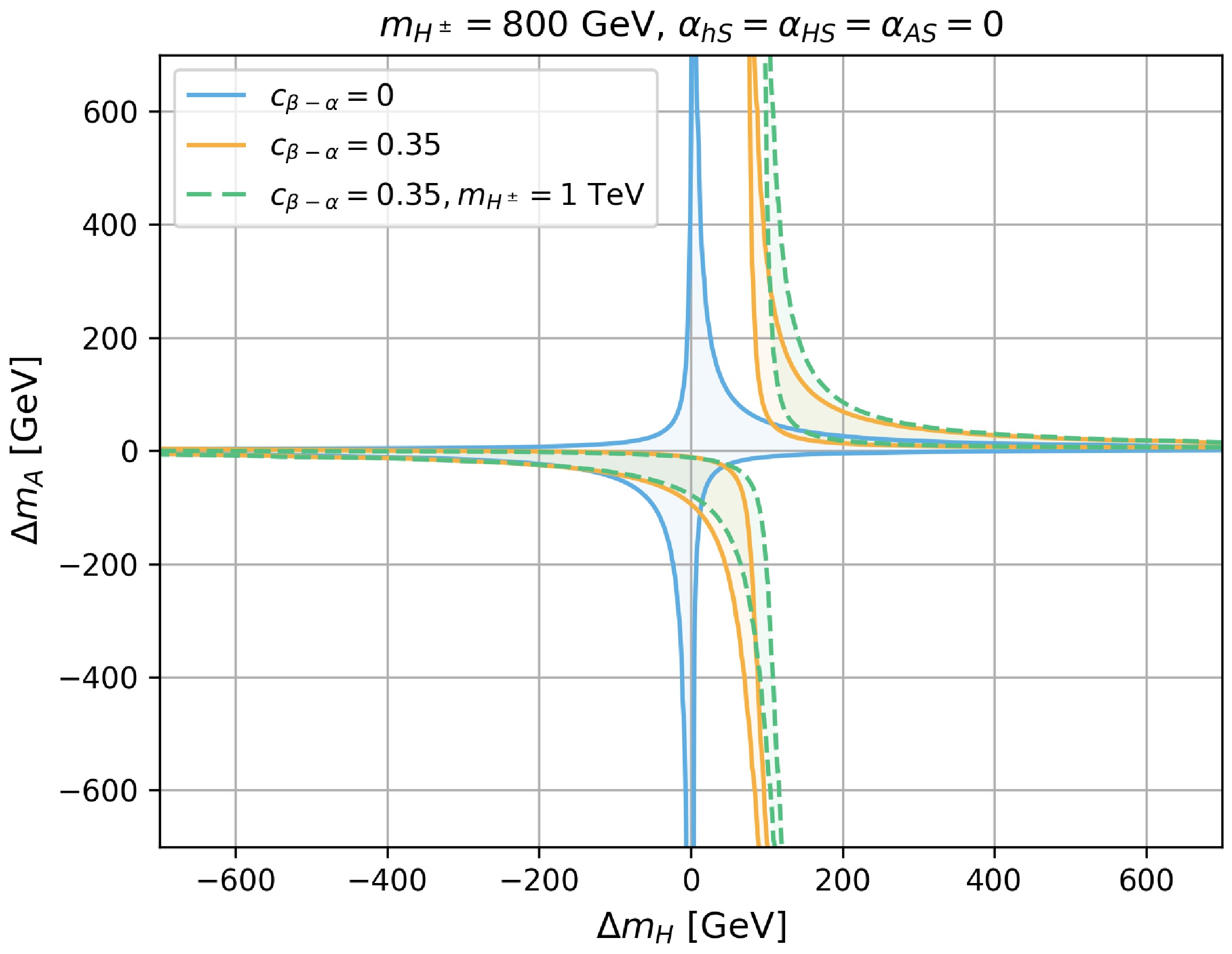
Figure 3. (color online) 95% C.L. allowed region from STU constraints in the plane
$ \Delta m_H $ vs.$ \Delta m_A $ with$ c_{\beta-\alpha}=0 $ (solid blue region) and$ 0.35 $ (solid orange region) for$ m_{H^\pm} = 800 $ GeV. The other parameters are$ \alpha_{HS}=\alpha_{hS}=\alpha_{AS}=0 $ . For$ m_{H^\pm} = 1000 $ GeV, the allowed region for$ c_{\beta-\alpha}=0 $ is approximately the same as that for$ m_{H^\pm} = 800 $ GeV, whereas the region for$ c_{\beta-\alpha}=0.35 $ is shown by the green regions.In Fig. 4, the 95% C.L. allowed regions under the STU constraints are shown in the
$ \Delta m_{A,H} $ vs.$ c_{\beta-\alpha} $ plane. For$ c_{\beta-\alpha}=0 $ , the 95% C.L. fit to the STU parameters gives$ \Delta m_{A,H} \lesssim 900 $ GeV with$ \Delta m_{H,A} = 0 $ for$ m_{H^\pm}=800 $ GeV (blue region). The upper limits on$ \Delta m_{A,H} $ come from the logarithm contributions. Note that a large mass difference can be allowed after theoretical considerations are taken into account, as long as$ m_{12} $ and other model parameters are allowed to vary within a certain range. These upper limits of$ \Delta m_{A,H} $ vary with the benchmark value of$ m_{H^\pm} $ and increase as$ {H^\pm} $ becomes heavier, as indicated by the green dashed curve for$ m_{H^\pm}=1000 $ GeV. For non-zero values of$ \Delta m_{A,H}=\pm 50 $ GeV, the allowed range of$ \Delta m_{H,A} $ is much smaller, as shown by the regions with the purple and orange boundary curves in Fig. 4.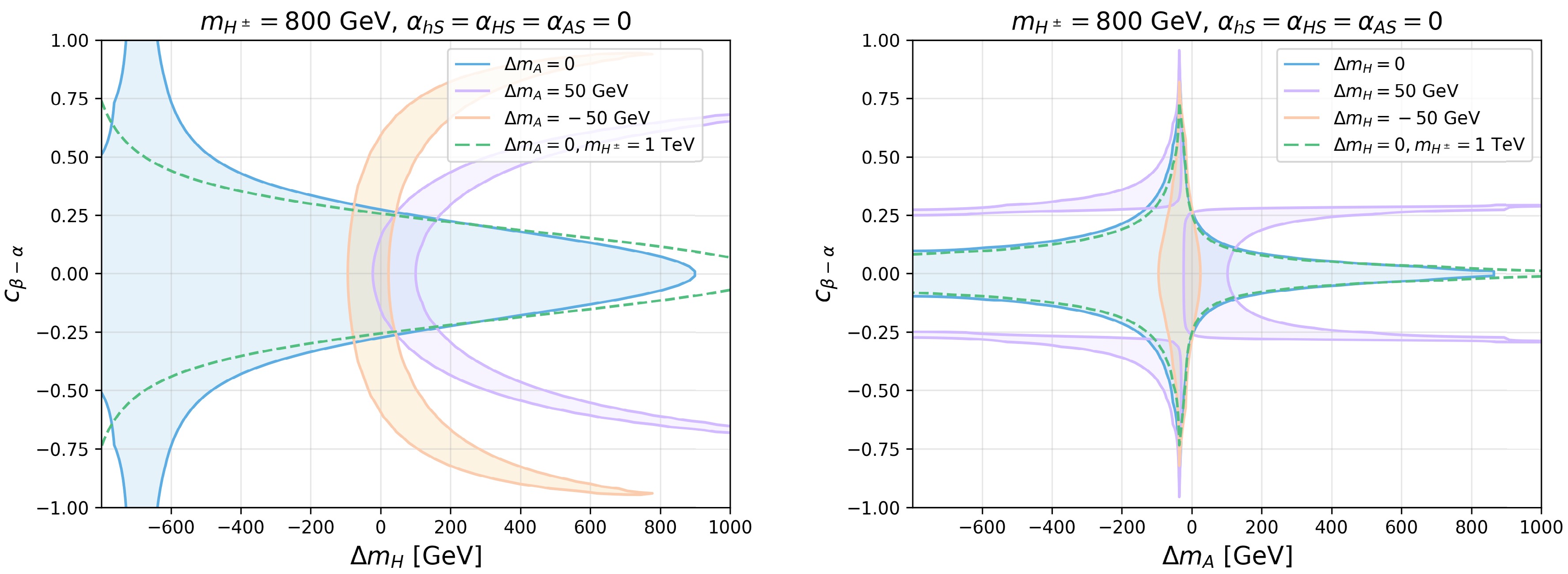
Figure 4. (color online) 95% C.L. allowed region via STU constraints on
$ c_{\beta-\alpha} $ vs.$ \Delta m_H $ (left) and$ \Delta m_A $ vs.$ c_{\beta-\alpha} $ (right). The other parameters are chosen as$ \alpha_{HS}=\alpha_{hS}=\alpha_{AS}=0 $ and$ m_H^\pm = 800 $ GeV (solid curves). The blue, purple, and orange regions correspond to$ \Delta m_{A,H}=0,\ 50,\ -50 $ GeV, respectively. The green dashed curves represent$ m_{H^\pm} = 1000 $ GeV and$ \Delta m_{A,H=0} $ . -
In Case-I (
$ c_{\beta-\alpha}\neq0 $ and$ \alpha_{HS}=\alpha_{hS}=\alpha_{AS}=0 $ ), the singlet fields decouple completely, and the model is the same as the 2HDM. In particular, we have the following non-zero couplings in addition to those shown in Eq. (19)$ \begin{aligned} c_{HVV},\;\;\; c_{AhZ}, \;\;\; c_{hH^\pm W^\mp}, \end{aligned} $
(22) which are proportional to
$ c_{\beta-\alpha} $ and provide additional contributions to the STU parameters. Similar to Case-0, the singlet masses$ m_{h_S} $ and$ m_{A_S} $ are irrelevant, and only the doublet-like Higgs masses$ m_H $ ,$ m_A $ , and$ m_{H^\pm} $ enter. The STU constraints of the 2HDM have been studied in the literature [26, 30]. The T observable in Case-I is$ \begin{aligned} T_{\rm{I}} &= T_0 + \Delta T_{\rm{I}} ,\end{aligned} $
(23) $ \begin{split} \Delta T_{\rm{I}}=\;& \frac{c^2_{\beta-\alpha}}{ 16\pi s^2_W m_W^2 } \{ F(m_h^2, m_{H^\pm}^2) - F (m_h^2, m_A^2) \\ &- [F(m_H^2, m_{H^\pm}^2) - F (m_H^2, m_A^2)] \\ &- 3 [F(m_h^2, m_{Z}^2) - F (m_h^2, m_{W^\pm}^2)] \\ &+ 3[F(m_H^2, m_{Z}^2) - F (m_H^2, m_{W^\pm}^2)] \} . \end{split} $
(24) Compared with Case-0, the additional contribution of
$ \Delta T_{\rm{I}} $ is proportional to$ c_{\beta-\alpha} $ , which is non-zero even for$ \Delta m_A = 0 $ .In Fig. 2, we show the values of
$ T_0 $ (solid curves) and$ \Delta T_{\rm{I}}/c_{\beta-\alpha}^2 $ (dashed curves) for different values of$ \Delta m_H $ and$ \Delta m_A $ . The left panel shows that, for$ \Delta m_H=-675 $ GeV, which corresponds to$ m_H= m_h=125 $ GeV,$ \Delta T_{\rm{I}} = 0 $ . The right panel shows that$ \Delta T_{\rm{I}} $ has the opposite (same) sign of$ T_0 $ for positive (negative)$ \Delta m_H $ , except for a small negative$ \Delta m_A $ region.The 95% C.L. STU allowed parameter space in the
$ \Delta m_H $ vs.$ \Delta m_A $ plane is shown in Fig. 3 for$ c_{\beta-\alpha}=0.35 $ (orange). The allowed regions shift to the right ($ \Delta m_H > 0 $ ), given the cancellation between$ T_0 $ and$ \Delta T_{\rm{I}} $ . In particular, the$ \Delta m_A = 0 $ point with$ \Delta m_H\sim $ 100 GeV and$ c_{\beta-\alpha}=0.35 $ would be excluded, as$ T_0 $ is zero and cannot eliminate the non-zero$ \Delta T_{\rm{I}} $ . The regions enclosed by the green dashed curves indicate$ m_{H^\pm}=1000 $ GeV, which is close to the orange regions of$ m_{H^\pm}=800 $ GeV.The left panel of Fig. 4 shows the 95% C.L. STU allowed parameter space in
$ c_{\beta-\alpha} $ vs.$ \Delta m_H $ for various$ \Delta m_A $ . The allowed regions are symmetric with respect to$ c_{\beta-\alpha}=0 $ , given the$ c_{\beta-\alpha}^2 $ dependence. For$ \Delta m_A=0 $ (region enclosed by the solid blue curve), all the values of$ c_{\beta-\alpha} $ are allowed at$ m_{H}=125 $ GeV:$ T_0=0 $ since$ \Delta m_A = 0 $ , and$ \Delta T_{\rm{I}}=0 $ for$ m_H = m_{h}=125 $ GeV. The allowed regions shrink for larger$ |m_H-m_{h_{125}}| $ . The green dashed line indicates the impact of the value of$ m_H^\pm $ . For non-zero$ \Delta m_A $ , the non-zero$ T_0 $ could be cancelled by$ \Delta T_{\rm{I}} $ . The allowed regions favor mostly positive$ \Delta m_H $ , as shown by the regions enclosed by the purple curves and orange curves. As the absolute value of$ \Delta T_{\rm{I}} $ is larger when$ \Delta m_A $ is positive as shown in Fig. 2, the allowed regions with positive$ \Delta m_A $ favor smaller$ |c_{\beta-\alpha}| $ . The 2HDM non-alignment case has been studied in [30], which did not cover the case with much larger mass splittings.The right panel of Fig. 4 shows the 95% C.L. STU allowed parameter space in
$ c_{\beta-\alpha} $ vs.$ \Delta m_A $ for various$ \Delta m_H $ . For$ \Delta m_H=0 $ (region enclosed by the solid blue curves), a relatively large region of$ c_{\beta-\alpha} $ is allowed for$ \Delta m_A \sim -30 $ GeV, when$ \Delta T_{\rm{I}} \sim 0 $ and$ S_0 $ and$ T_0 $ are small. The allowed regions of$ c_{\beta-\alpha} $ for$ \Delta m_A >0 $ are smaller than those for$ \Delta m_A <0 $ , as$ |\Delta T_{\rm{I}}| $ is larger for positive$ \Delta m_A $ . Note that, for negative$ \Delta m_H=-50 $ GeV, only a narrow range of$ \Delta m_A $ around$ -30 $ GeV is allowed. This is because$ \Delta T_{\rm{I}} $ has the same signs as$ T_0 $ for negative$ \Delta m_H $ . Therefore, only small values of$ \Delta m_A $ are allowed. However, for positive$ \Delta m_H=50 $ GeV,$ \Delta T_{\rm{I}} $ and$ T_0 $ have opposite signs. A wide range of$ \Delta m_A $ is allowed:$ |c_{\beta-\alpha}|\lesssim 0.25 $ for$ \Delta m_A>0 $ , and$ |c_{\beta-\alpha}| \gtrsim 0.25 $ for$ \Delta m_A<0 $ . -
In Case-II (e.g.,
$ \alpha_{hS}\neq0 $ and$ c_{\beta-\alpha}=\alpha_{HS}=\alpha_{AS}=0 $ ), the 125 GeV Higgs h mixes with the singlet-like Higgs$ h_S $ , and the$ h_S VV $ coupling is proportional to$ s_{\alpha_{hS}} $ , which is the only non-zero trilinear coupling between Higgs and gauge bosons, in addition to those in Eq. (19). The$ A h_S Z $ and$ h_S H^\pm W^\mp $ couplings are still zero, which indicates that$ \alpha_{hS} $ cannot connect the$ h_S $ with the BSM doublet-like Higgses H, A, or$ H^\pm $ . This case is similar to the singlet extension of the SM (SSM), where the singlet Higgs only mixes with the SM Higgs h. Therefore, the STU parameters receive additional contribution via loops with$ h_SVV $ vertices, with the singlet Higgs mass$ m_{h_S} $ entering. The S and T parameters are given by$ \begin{aligned} & S_{\rm{II}}= S_0+\Delta S_{\rm{II}},\ \ \ T_{\rm{II}}=T_0 + \Delta T_{\rm{II}}, \end{aligned} $
(25) $ \begin{split} \Delta S_{\rm{II}}=\;&\frac{1}{24\pi}s^2_{\alpha_{hS}} \Big[ \ln \left( \frac{m_{h_S}^2}{m_{h_{125}}^2}\right) + \hat{G}(m_{h_S}^2, m_Z^2)\\ &- \hat{G}(m_{h_{125}}^2, m_Z^2) \Big], \end{split} $
(26) $ \begin{split} \Delta T_{\rm{II}}=\;&\frac{1}{16\pi s_W^2 m_W^2}3s^2_{\alpha_{hS}}\Big[F(m_Z^2,m_{h_S}^2)-F(m_W^2,m_{h_S}^2) \\ &- F(m_Z^2,m_{h_{125}}^2)+F(m_W^2,m_{h_{125}}^2) \Big]. \end{split} $
(27) The expression for the function
$ \hat{G} $ can be found in Eq. (A6). Note that$ \Delta T_{\rm{II}} $ and$ \Delta S_{\rm{II}} $ are proportional to$ s^2_{\alpha_{hS}} $ , and both terms vanish when$ m_{h_S}=m_{h_{125}} $ .$ \Delta S_{\rm{II}} $ is, in general, suppressed, whereas$ \Delta T_{\rm{II}} $ could receive a significant contribution when$ m_{h_S} $ is away from 125 GeV, which is negative (positive) for$ m_{h_S}> (<) $ 125 GeV. Meanwhile, the masses of H, A, or$ H^\pm $ can still contribute via$ T_0 $ and$ S_0 $ .In the left panel of Fig. 5, we show the 95% C.L. allowed region from the STU constraints in the
$ m_{h_S} $ vs.$ \alpha_{hS} $ plane for different values of$ \Delta m_H = \Delta m_A $ . For$ \Delta m_H = \Delta m_A=0 $ (blue), all values of$ \alpha_{hS} $ are allowed for$ m_{h_S}=m_h \approx 125 $ GeV. The allowed region for$ \alpha_{hS} $ reduces for$ m_{h_S} $ away from 125 GeV:$ |\alpha_{hS}|\lesssim 0.7 $ for light$ m_{h_S}=10 $ GeV and$ |\alpha_{hS}|\lesssim 0.2 $ for$ m_{h_S}=1 $ TeV.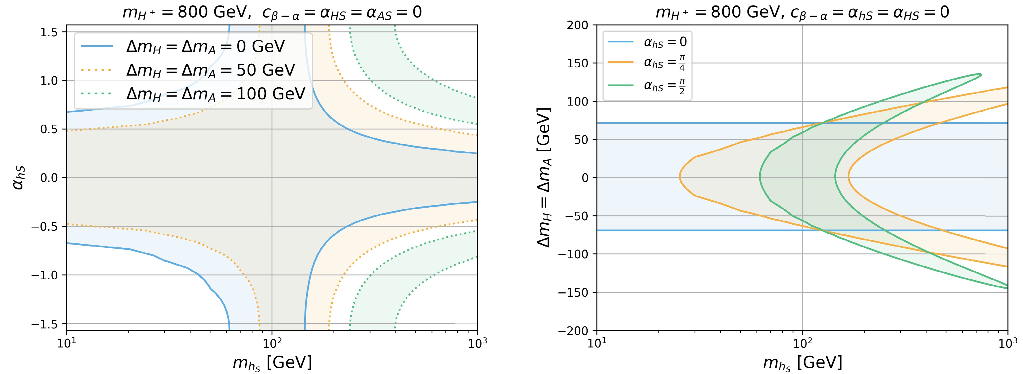
Figure 5. (color online) 95% C.L. STU constraints on the parameter space of
$ m_{h_S} $ ,$ \alpha_{hS} $ , and$ \Delta m_A $ . The left panel indicates$ m_{h_S} $ vs.$ \alpha_{hS} $ with varying$ \Delta m_A $ . The blue, orange, and green regions indicate$ \Delta m_A = \Delta m_H=0 $ , 50, 100 GeV, respectively. The right panel indicates$ m_{h_S} $ vs.$ \Delta m_{H,A} $ with varying$ \alpha_{hS} $ . The blue, orange, and green regions indicate$ \alpha_{hS}=0 $ ,$ {\pi}/{4} $ , and$ {\pi}/{2} $ , respectively. For both panels, we set$ m_{H^\pm}= 800 $ GeV and$ c_{\beta-\alpha}=\alpha_{HS}=\alpha_{AS}=0 $ .For
$ \Delta m_H = \Delta m_A=50 $ GeV (orange), the 95% C.L. allowed region shifted to the right of$ m_{h_S}=125 $ GeV, owing to the opposite signs of$ T_0 $ and$ \Delta T_{\rm{II}} $ for$ m_{h_S}>125 $ GeV. For$ \Delta m_H = \Delta m_A=100 $ GeV (green),$ T_0 $ is so large that only two thin branches in$ m_{h_S}>240 $ GeV and$ 0.5<|\alpha_{hS}|<\pi/2 $ are allowed.In the right panel of Fig. 5, we show the 95% C.L. STU allowed region in the
$ m_{h_S} $ vs.$ \Delta m_{H,A} $ plane for$ \alpha_{hS}=0 $ (blue),$ \pi/4 $ (orange), and$ \pi/2 $ (green). For$ \alpha_{hS}=0 $ , the bound of$ |\Delta m_{H}|=|\Delta m_A |\lesssim $ 80 GeV is independent of$ m_{h_S} $ . For non-zero$ \alpha_{hS} $ , the allowed value in$ |\Delta m_{H,A}| $ reduces for$ m_{h_S}<125 $ GeV but increases for$ m_{h_S}>125 $ GeV. Note that all curves cross at$ m_{h_S}=125 $ GeV, as$ \Delta T_{\rm{II}} $ and$ \Delta S_{\rm{II}} $ vanish at$ m_{h_S}=125 $ GeV regardless of the value of$ \alpha_{hS} $ . There is a slight asymmetry between the positive and negative values of$ \Delta m_H=\Delta m_A $ . This is because the$ S_0 $ observable is not symmetric between positive and negative$ \Delta m_{H,A} $ .$ \Delta S_{\rm{II}} $ is always positive for$ m_{h_S}> m_{h_{125}} $ , whereas the sign of$ S_0 $ flips for different signs of$ \Delta m_{H,A} $ . Therefore, the S observable is larger for positive$ \Delta m_{H,A} $ and the constraint would be stronger, which leads to the allowed region for$ \Delta m_{H,A}>0 $ being slightly smaller than that in the negative mass difference case. -
Case-III corresponds to
$ \alpha_{HS}\neq0 $ and$ c_{\beta-\alpha}=\alpha_{hS}= \alpha_{AS}=0 $ , when$ h_S $ mixes with the doublet-like CP-even Higgs H. The non-zero trilinear Higgs to gauge-boson couplings include$ \begin{aligned} c_{Ah_S Z},\quad c_{h_S H^\pm W^\mp}, \end{aligned} $
(28) in addition to those in Eq. (19). However, the
$ h_S VV $ coupling remains zero in this case. While the additional contribution to the S observable is small, the T observable could receive significant contributions:$ \begin{split} T=\;&\frac{1}{16\pi s_W^2 m_W^2} [c_{\alpha_{HS}}^2 F(m_{H^\pm}^2, m_H^2) +s^2_{\alpha_{HS}}F(m_{H^\pm}^2, m_{h_S}^2) ]\\ & + F(m_{H^\pm}^2, m_A^2) - [c_{\alpha_{HS}}^2 F(m_{A}^2, m_H^2) + s^2_{\alpha_{HS}} F(m_{A}^2, m_{h_S}^2) ] . \end{split} $
(29) $ \begin{aligned} = &T_0 + \Delta T_{\rm{III}}, \end{aligned} $
(30) $ \begin{split} \Delta T_{\rm{III}} =\;& \frac{ s_{\alpha_{HS}}^2}{16\pi s_W^2 m_W^2}[ F(m_{H^\pm}^2, m_{h_S}^2) - F(m_{A}^2, m_{h_S}^2)\\ &- F(m_{H^\pm}^2, m_{H}^2) + F(m_{A}^2, m_{H}^2) ]. \end{split} $
(31) In addition to
$ \Delta m_{H,A} $ ,$ \Delta m_{h_S}=m_{h_S}-m_{H^\pm} $ enters.There is a numerical approximation for the F function in Eq. (A4):
$ \begin{split} &c_{\alpha}^2 [F(J^2,I^2) - F(K^2,I^2)] + s_{\alpha}^2 [F(J^2,L^2)-F(K^2,L^2)] \\ \approx & F( J^2, [c_\alpha^2 I + s_\alpha^2 L]^2) -F(K^2, [c_\alpha^2 I + s_\alpha^2 L]^2). \end{split} $
(32) Therefore, the T observable can be approximated as
$ \begin{split} T\approx\;& \frac{ 1}{16\pi s_W^2 m_W^2} [F(m_{H^\pm}^2, (c_{\alpha_{HS}}^2 m_H + s^2_{\alpha_{HS}}m_{h_S})^2) \\ &- F(m_{A}^2, (c_{\alpha_{HS}}^2 m_H + s^2_{\alpha_{HS}} m_{h_S})^2) + F(m_{H^\pm}^2, m_A^2) ] \end{split} $
(33) which vanishes for
$ \begin{aligned} c^2_{\alpha_{HS}} m_H+ s^2_{\alpha_{HS}}m_{h_S} = m_{H^\pm} ,\ \ \ {\rm{or}}\ \ \ m_A=m_{H^\pm}. \end{aligned} $
(34) Figure 6 presents the 95% STU allowed region in the
$ \Delta m_H $ vs.$ \Delta m_A $ plane for Case-III. The region enclosed by the dark blue curves corresponds to the baseline Case-0 when$ \alpha_{HS}=0 $ . For$ \alpha_{HS}=\pi/4 $ and$ \Delta m_{hS}=0 $ (region enclosed by the light dotted blue lines), the 95% C.L. STU allowed region would be slightly enlarged compared with that in Case-0, as the mass-splitting effect of H with$ H^\pm $ is suppressed by$ c^2_{\alpha_{HS}}=1/2 $ , whereas$ h_S $ has no mass splitting with the charged Higgs, as shown in Eq. (34).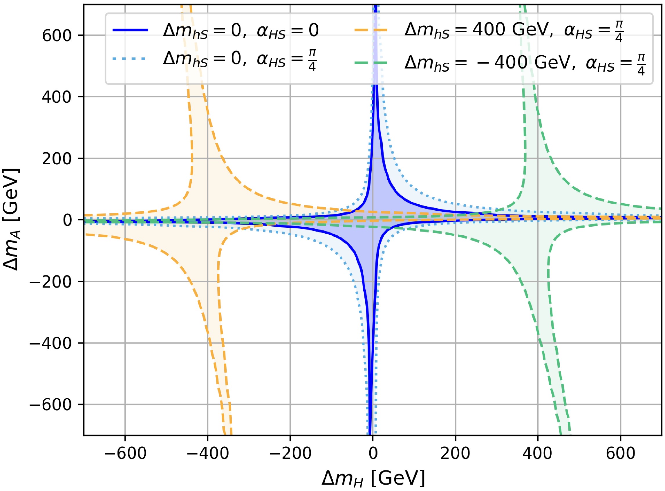
Figure 6. (color online) 95% C.L. STU allowed region in
$ \Delta m_H $ vs.$ \Delta m_A $ in Case-III with$ c_{\beta-\alpha}=\alpha_{hS}=\alpha_{AS}=0 $ .$ m_{H^\pm} $ is set to be 800 GeV. The regions enclosed by the dark solid blue and light dashed blue curves indicate$ \Delta m_{hS}=0 $ and$ \alpha_{HS}=0 $ and$ \pi/4 $ , respectively. The orange and green regions indicate$ \Delta m_{hS}=\pm $ 400 GeV, respectively, and$ \alpha_{HS}=\pi/4 $ .When the singlet-like Higgs mass deviates from the charged Higgs mass, for instance,
$ \Delta m_{hS}=\pm 400 $ GeV with$ \alpha_{HS}= {\pi}/{4} $ , as shown by the orange and green regions, the center of the allowed region in$ \Delta m_H $ shifts to the region of$ \Delta m_H\approx \mp 400 $ GeV to satisfy the mass relation in Eq. (34) to suppress the contributions to the T parameter. Note that$ \Delta m_A=0 $ is still allowed, regardless of the choices of$ \Delta m_H $ ,$ \Delta m_{h_S} $ , and$ \alpha_{HS} $ .In the left panel of Fig. 7, we show the 95% C.L. STU allowed region in the
$ \Delta m_H $ vs.$ \Delta m_{hS} $ plane in Case-III for$ m_{H^\pm}=800 $ GeV and$ \Delta m_A=200 $ GeV, with varying$ \alpha_{HS}=0 $ (blue),$ \pi/6 $ (orange), and$ \pi/4 $ (green). The dashed lines show the approximate relation of$ c^2_{\alpha_{HS}}\Delta m_H= -s^2_{\alpha_{HS}} \Delta m_{hS} $ based on Eq. (34). The approximation is valid for$ \Delta m_H $ and$ \Delta m_{hS} $ around a few hundred GeV. As the mass splitting$ \Delta m_A $ increases, the STU bands would shrink and be closer to the dashed lines.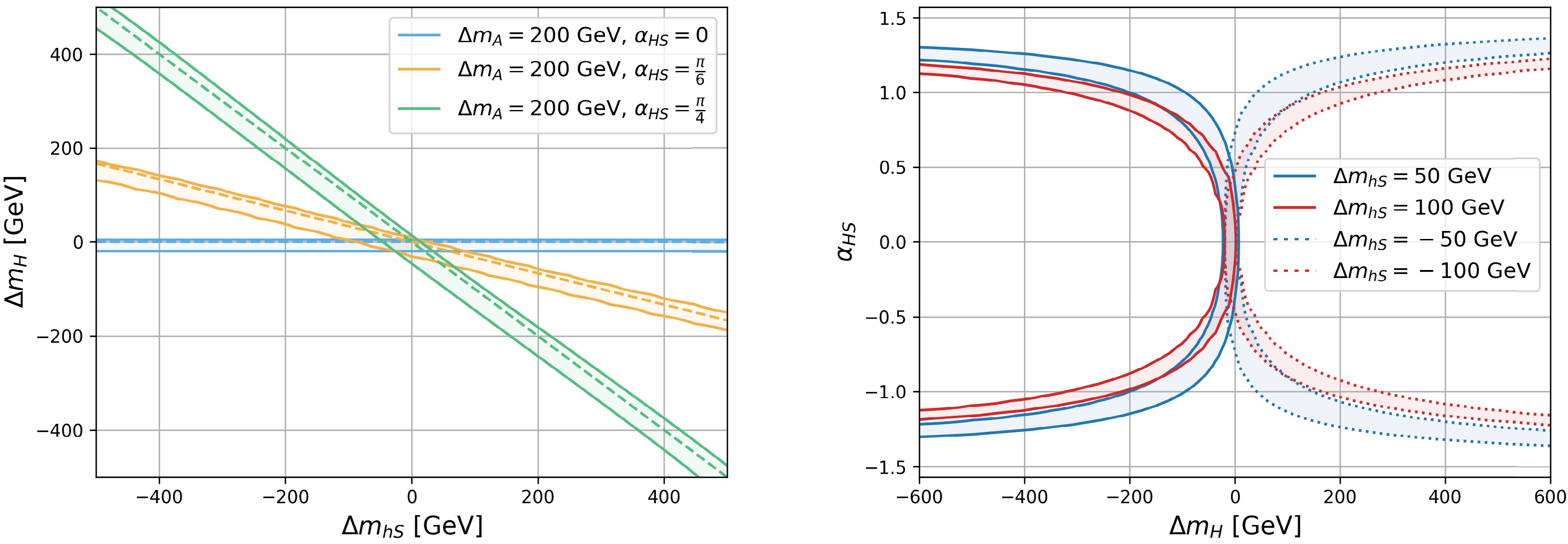
Figure 7. (color online) 95% C.L. STU allowed region in
$ \Delta m_H $ vs.$ \Delta m_{hS} $ plane (left panel) and$ \Delta m_{H} $ vs.$ \alpha_{HS} $ plane (right panel) in Case-III with$ c_{\beta-\alpha}=\alpha_{hS}=\alpha_{AS}=0 $ . In the left panel,$ \alpha_{HS} $ is varied to be 0 (blue),$ \pi/6 $ (orange), and$ \pi/4 $ (green). In the right panel,$ \Delta m_{hS} $ is varied to be$ \pm 50 $ GeV (solid and dashed blue) and$ \pm 50 $ GeV (solid and dashed red).$ m_{H^\pm} $ is set to be 800 GeV, and$ \Delta m_A $ is set to be 200 GeV.In the right panel of Fig. 7, we show the 95% C.L. STU allowed region in the
$ \Delta m_H $ vs.$ \alpha_{HS} $ plane in Case-III for$ m_{H^\pm}=800 $ GeV and$ \Delta m_A=200 $ , with varying$ \Delta m_{hS}=\pm 50 $ GeV (blue) and 100 GeV (red). Note that the allowed regions are symmetric in$ \alpha_{HS} $ and only have a slight variation with respect to the sign of$ \Delta m_H $ . -
In Case-IV, (
$ \alpha_{AS}\neq0 $ and$ c_{\beta-\alpha}=\alpha_{hS}=\alpha_{HS}=0 $ ), the CP-odd sector has singlet admixture, and the CP-even sector is the same as that in Case-0. The non-zero trilinear Higgs to gauge-boson couplings include$ \begin{aligned} \; c_{A_S H Z},\quad c_{A_S H^\pm W^\mp}, \end{aligned} $
(35) in addition to those in Eq. (19). Consequently, the couplings involving CP-odd Higgses are parameterized by
$ \alpha_{AS} $ , i.e., AHZ and$ AH^\pm W^\mp $ depend on$ c_{\alpha_{AS}} $ , and$ A_S HZ $ and$ A_S H^\pm W^\mp $ depend on$ s_{\alpha_{AS}} $ . The singlet CP-odd Higgs mass$ m_{A_S} $ enters, whereas the CP-even$ {h_S} $ is completely decoupled. In particular, the contribution to the T observable is given by$ \begin{split} T=\;&\frac{1}{16\pi s_W^2 m_W^2} [c_{\alpha_{AS}}^2 F(m_{H^\pm}^2, m_A^2) +s^2_{\alpha_{AS}}F(m_{H^\pm}^2, m_{A_S}^2) ]\\ & + F(m_{H^\pm}^2, m_H^2) - [c_{\alpha_{AS}}^2 F(m_{H}^2, m_A^2) + s^2_{\alpha_{AS}} F(m_{H}^2, m_{A_S}^2) ] , \end{split} $
(36) $ \begin{aligned} =& T_0 + \Delta T_{\rm{IV}} \end{aligned} $
(37) $ \begin{split} \Delta T_{\rm{IV}} =\;& \frac{ s_{\alpha_{AS}}^2}{16\pi s_W^2 m_W^2}[ F(m_{H^\pm}^2, m_{A_S}^2) - F(m_{H}^2, m_{A_S}^2)\\ &- F(m_{H^\pm}^2, m_{A}^2) + F(m_{A}^2, m_{H}^2) ] .\end{split} $
(38) Comparing with Eqs. (29) and (31), we observe that Case-IV is similar to Case-III, with the substitution of H and
$ h_S $ with A and$ A_S $ , as well as the corresponding mass parameters and mixing angles. The approximate expression for T is$ \begin{split} T\approx \;&\frac{ 1}{16\pi s_W^2 m_W^2} [F(m_{H^\pm}^2, (c_{\alpha_{AS}}^2 m_A + s^2_{\alpha_{AS}}m_{A_S})^2) \\ &- F(m_{H}^2, (c_{\alpha_{AS}}^2 m_A + s^2_{\alpha_{AS}} m_{A_S})^2) + F(m_{H^\pm}^2, m_H^2) ], \end{split} $
(39) which leads to a similar approximate mass relation that satisfies the STU constraints:
$ \begin{aligned} c^2_{\alpha_{AS}} m_A + s^2_{\alpha_{AS}}m_{A_S} = m_{H^\pm}, \ \ \ {\rm{or}}\quad m_H=m_{H^\pm}. \end{aligned} $
(40) The 95% C.L. STU allowed regions in
$ \Delta m_H $ vs.$ \Delta m_A $ ,$ \Delta m_{AS} $ vs.$ \Delta m_A $ , and$ \Delta m_A $ vs.$ \alpha_{AS} $ are similar to those presented in Figs. 6−7, with the switching of$ A\leftrightarrow H $ .In general, the mass splittings of
$ \Delta m_H $ and$ \Delta m_A $ can contribute the STU observables via the AHZ,$ AH^\pm W^\mp $ , and$ H H^\pm W^\mp $ loops. In the 2HDM+S, the singlet CP-even Higgs$ h_S $ can mix with H via the mixing$ \alpha_{HS} $ , and the singlet CP-odd Higgs$ A_S $ can mix with$ A_S $ via$ \alpha_{AS} $ . Therefore,$ \Delta m_{hS} $ and$ \Delta m_{AS} $ as well as$ \alpha_{HS} $ and$ \alpha_{AS} $ enter. The STU constraints can be still fulfilled when the mass relations in Eqs. (34) or (40) are satisfied. -
For Case-I, we consider the non-alignment limit with all the single mixing angles set to be zero. For Cases-II − IV, we focus on the scenario with only one mixing angle set to be non-zero under the alignment limit. In this section, we consider the cases with a non-zero singlet mixing angle beyond the alignment limit.
We first explore the interplay between
$ c_{\beta-\alpha} $ with the singlet−$ h_{125} $ mixing$ \alpha_{hS} $ . In the left plot of Fig. 8, we show the 95% C.L. STU allowed region in the$ m_{h_S} $ vs.$ c_{\beta-\alpha} $ plane for various$ \alpha_{hS} $ . For$ \alpha_{hS}=0 $ (region enclosed by the solid blue curve),$ |c_{\beta-\alpha}| $ is constrained to be less than 0.275, independent of$ m_{h_S} $ . However, the singlet admixture can enlarge the allowed region in$ |c_{\beta-\alpha}| $ , as shown by the two elliptical rings for$ \alpha_{hS}=\pi/4 $ and$ \pi/2 $ . The$ h_SVV $ interaction can compensate for the contribution of$ \Delta T_{\rm{I}} $ in Eq. (24) for larger$ |c_{\beta-\alpha}| $ .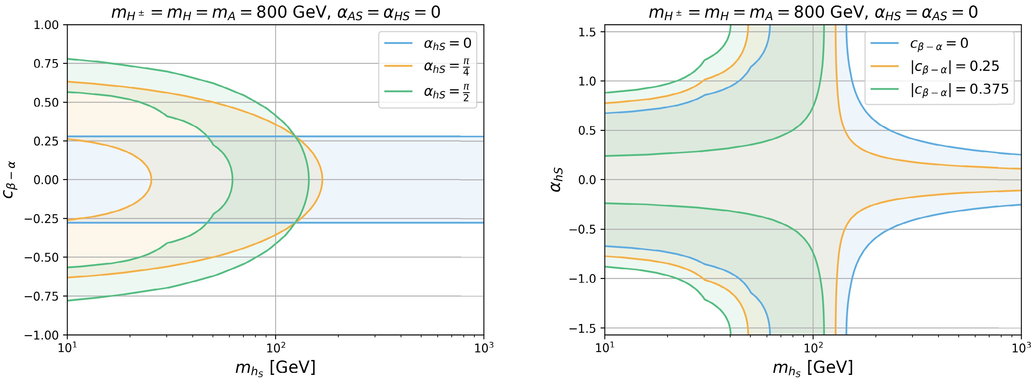
Figure 8. (color online) 95% C.L. STU allowed region in the
$ m_{h_S} $ vs.$ c_{\beta-\alpha} $ plane (left panel) for$ \alpha_{hS}=0 $ (blue),$ \pi/4 $ (orange), and$ \pi/2 $ (green) and the$ m_{h_S} $ vs.$ \alpha_{hS} $ plane (right panel) for$ c_{\beta-\alpha}=0 $ (blue), 0.25 (orange), and 0.375 (green). We set$ m_{H^\pm}=m_{H}=m_A=800 $ GeV and$ \alpha_{AS}=\alpha_{HS}=0 $ .In the right plot of Fig. 8, we present the 95% C.L. STU allowed region in the
$ m_{h_S} $ vs.$ \alpha_{hS} $ plane for various$ c_{\beta-\alpha} $ . For increasing$ |c_{\beta-\alpha}| $ , the allowed region shifts to the left. For$ m_{h_S}>125 $ GeV, the allowed range of$ \alpha_{hS} $ reduces, whereas for$ m_{h_S}<125 $ GeV, larger values of$ \alpha_{hS} $ are allowed. For$ |c_{\beta-\alpha}| $ slightly above 0.275,$ \alpha_{hS}=0 $ is no longer allowed, and two branches appear.We explore the interplay between
$ c_{\beta-\alpha} $ and singlet-double CP-even Higgs H mixing$ \alpha_{HS} $ in Fig. 9. The left panel shows the 95% C.L. STU allowed region in the$ \Delta m_{H} $ vs.$ c_{\beta-\alpha} $ plane for$ \alpha_{HS}=0 $ (blue),$ \pi/4 $ (orange), and$ \pi/2 $ (green). The blue line in the left panel of Fig. 9 is consistent with the blue curve in the left panel of Fig. 4 (Case-I). For larger$ \alpha_{HS} $ , the allowed range of$ c_{\beta -\alpha} $ shrinks for$ \Delta m_H < 0 $ but expands for$ \Delta m_H > 0 $ . In this case,$ c_{HVV} = c_{\beta-\alpha}c_{\alpha_{HS}} $ ,$ c_{hVV} = s_{\beta-\alpha} $ , and$ c_{h_SVV} = -c_{\beta-\alpha}s_{\alpha_{HS}} $ . As$ \alpha_{HS} $ increases, the HVV contribution to the T observable decreases, whereas the$ h_SVV $ contribution increases. Therefore, the allowed$ c_{\beta-\alpha} $ region shrinks in the$ h_SVV $ dominate region ($ m_H<m_{h_S} $ ) and enlarges in the HVV dominate region ($ m_H>m_{h_S} $ ). When$ m_H=m_{h_S}= $ 800 GeV, the$ h_SVV $ term plays the same role as HVV. The$ STU $ constraints of this point are independent of$ \alpha_{HS} $ and all curves cross at$ \Delta m_H=0 $ . For$\alpha_{HS}= {\pi}/{2}$ , H becomes the pure singlet Higgs and does not contribute to the STU parameters. Therefore, the STU limit of$ |c_{\beta-\alpha}|<0.275 $ is independent of$ m_H $ . As the roles of H and$ h_S $ switch when$ \alpha_{HS} \rightarrow \pi/ 2-\alpha_{HS} $ , the parameter space of$ c_{\beta-\alpha} $ vs.$ \Delta m_{h_S} $ is the same as that of the left panel of Fig. 9 with$ \alpha_{HS}\rightarrow \pi/2-\alpha_{HS} $ .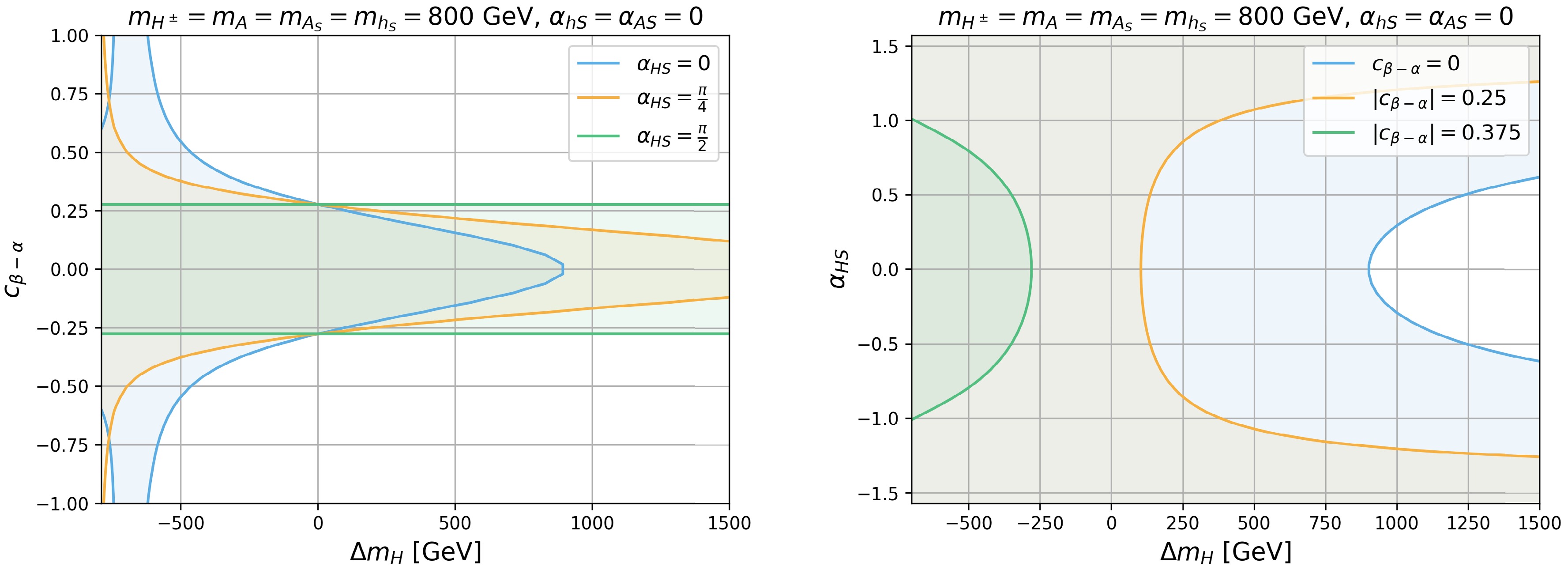
Figure 9. (color online) 95% C.L. STU allowed region in the
$ \Delta m_{H} $ vs.$ c_{\beta-\alpha} $ plane (left panel) for$ \alpha_{HS} $ =0 (blue),$ \pi/4 $ (orange), and$ \pi/2 $ (green) and the$ \Delta m_{H} $ vs.$ \alpha_{HS} $ plane (right panel) for$ |c_{\beta-\alpha}| $ =0 (blue), 0.25 (orange), and 0.375 (green). We set$ m_{H^\pm}=m_A= m_{h_S}= $ $ m_{A_S}=800 $ GeV and$ \alpha_{AS}=\alpha_{hS}=0 $ .The right panel of Fig. 9 presents the
$ \Delta m_{H} $ vs.$ \alpha_{HS} $ plane for$ |c_{\beta-\alpha}| $ =0 (blue), 0.25 (orange), and 0.375 (green). For$ c_{\beta-\alpha}=0 $ , almost the entire region of the parameter space is allowed, except for a small open region with relatively small$ \alpha_{HS} $ and large$ \Delta m_H $ . The allowed region reduces when$ |c_{\beta-\alpha}| $ increases. For$ |c_{\beta-\alpha}|=0.375 $ , only a small region with$ \Delta m_H<-250 $ GeV and$ |\alpha_{HS}|<1 $ is allowed. This is due to the increased contribution from the HVV term at larger$ |c_{\beta-\alpha}|=0.375 $ . Only when$ m_H $ is lighter and close to 125 GeV would the HVV contribution be small enough to be allowed. Similar to the left panel, the parameter space of$ \alpha_{HS} $ vs.$ \Delta m_{h_S} $ is the same as that of the right panel of Fig. 9 with$ \alpha_{HS}\rightarrow \pi/2-\alpha_{HS} $ .We explore the interplay between
$ c_{\beta-\alpha} $ and singlet-double CP-odd Higgs A mixing$ \alpha_{AS} $ in Fig. 10. The left panel presents the 95% C.L. allowed region in$ \Delta m_A $ vs.$ c_{\beta-\alpha} $ for$ \alpha_{HS} $ =0 (blue),$ \pi/4 $ (orange), and$ \pi/2 $ (green). The blue region in the left panel of Fig. 10 for$ \alpha_{AS}=0 $ is consistent with the blue region in the right panel of Fig. 4. For larger$ \alpha_{AS} $ , the allowed regions shift to the left, whereas the$ c_{\beta-\alpha} $ bounds at both$ m_{A}>m_{A_S} $ and$ m_{A}<m_{A_S} $ become larger, owing to the suppression of both the$ A H Z $ and$ AhZ $ terms by$ c_{\alpha_{AS}} $ . However, the$ A_S hZ $ term is enhanced by$ s_{\alpha_{AS}} $ , which compensates for the suppression of$ A H Z $ and$ AhZ $ . Therefore, the STU limit is relaxed faster at$ m_{A}>m_{A_S} $ where$ A_S $ is less dominant in this region. For$ \alpha_{AS}=\pi/2 $ , only the$ A_S h Z $ contribution is left, and the contribution from A is decoupled. The 95% C.L. allowed region for the$ c_{\beta-\alpha} $ limit is a constant and independent of$ m_A $ . As the roles of A and$ A_S $ switch when$ \alpha_{AS} \rightarrow \pi/ 2-\alpha_{AS} $ , the parameter space of$ c_{\beta-\alpha} $ vs.$ \Delta m_{A_S} $ is the same as that in the left panel of Fig. 10 with$ \alpha_{AS}\rightarrow \pi/2-\alpha_{AS} $ .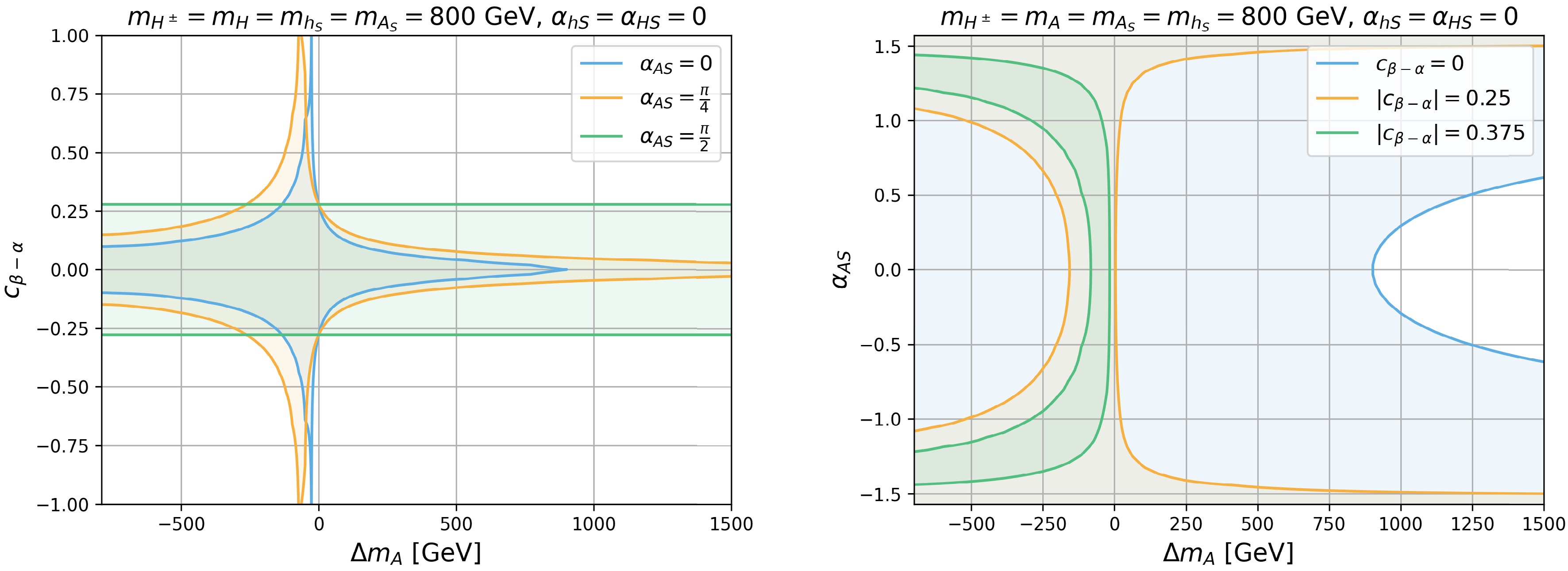
Figure 10. 95% C.L. STU allowed region in the
$ \Delta m_{A} $ vs.$ c_{\beta-\alpha} $ plane (left panel) for$ \alpha_{HS} $ =0 (blue),$ \pi/4 $ (orange), and$ \pi/2 $ (green) and the$ \Delta m_{A} $ vs.$ \alpha_{AS} $ plane (right panel) for$ |c_{\beta-\alpha}| $ =0 (blue), 0.25 (orange), and 0.375 (green). We set$ m_{H^\pm}=m_H=m_{h_S}=m_{A_S}=800 $ GeV and$ \alpha_{hS}=\alpha_{HS}=0 $ .The right panel of Fig. 10 presents the 95% C.L. allowed region in
$ \Delta m_A $ vs.$ \alpha_{AS} $ for$ |c_{\beta-\alpha}| $ =0 (blue), 0.25 (orange), and 0.375 (green). The blue line indicates the same behavior of the STU dependence on$ (m_A, \alpha_{AS}) $ as$ (m_H, \alpha_{HS}) $ for$ c_{\beta-\alpha}=0 $ . However, these two cases differ when singlet admixture enters for$ c_{\beta-\alpha} \neq 0 $ . The CP-odd Higgs A enters via$ A h Z $ and$ A HZ $ s, where these contributions are suppressed when$ m_{A} $ is close to$ m_H $ . In the case where$ m_{A_S}=m_H $ , the allowed regions that only appear in the region of large$ \alpha_{AS} $ are non-zero$ \Delta m_A $ , as$ A_S $ in this area is already dominated by the doublet properties. Similar to the left panel, the parameter space of$ \alpha_{AS} $ vs.$ \Delta m_{A_S} $ is the same as that in the right panel of Fig. 10 with$ \alpha_{AS}\rightarrow \pi/ 2-\alpha_{AS} $ . -
The precision measurements of the couplings of the 125 GeV Higgs at the LHC also place strong constraints on the parameter space of the 2HDM+S, in particular, on
$ c_{\beta-\alpha} $ , the singlet-$ h_{125} $ mixing$ \alpha_{hS} $ , and$ \tan\beta $ . We perform the fit for 125 GeV Higgs properties with$\mathrm{HiggsTools} $ [31−35]. In Fig. 11, we present both the 95% C.L. STU allowed region in the$ c_{\beta-\alpha} $ vs.$ \alpha_{hS} $ plane for various$ m_{h_S} $ (regions enclosed by solid curves) and the 95% C.L. allowed region by 125 GeV Higgs precision measurements for various$ \tan\beta $ (region enclosed by dashed curves) for Type-I (left panel) and Type-II (right panel). As the STU constraints only depend on the couplings of the Higgses with the gauge bosons, which is the same for different types of 2HDM, the solid curves are the same at both panels. For$ m_{h_S}=125 $ GeV, the allowed range in$ c_{\beta-\alpha} $ is independent of$ \alpha_{hS} $ . This is because$ h_SVV $ and$ hVV $ contribute the same for$ m_{h}=m_{h_S} $ , and$ \alpha_{hS} $ is not constrained as shown in the left plot of Fig. 5. For$ m_{h_S}=50 $ GeV, a larger region of$ c_{\beta-\alpha} $ can be accommodated for$ \alpha_{h_S} \neq 0 $ , as a larger$ \Delta T_{\rm{I}} $ can be compensated for by$ h_SVV $ with lighter$ m_{h_S} $ . In contrast, for$ m_{h_S}>125 $ GeV, the allowed region in$ \alpha_{h_S} $ shrinks, where$ \Delta T_{\rm{I}} $ and$ h_S VV $ have the same sign in this mass region, which leads to tighter constraints.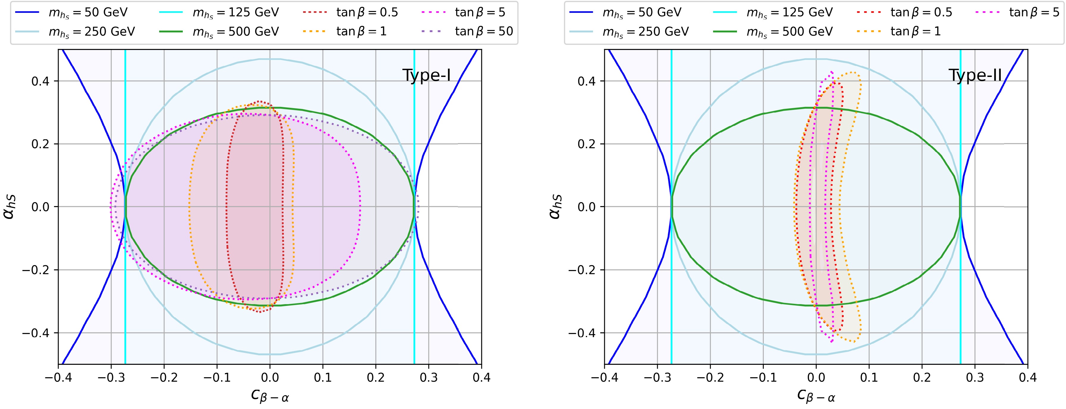
Figure 11. Parameter space of
$ c_{\beta-\alpha} $ vs.$ \alpha_{hS} $ for$ m_{h_S}= $ 50 GeV (dark blue), 125 GeV (cyan), 250 GeV (light blue), and 500 GeV (green) and$ \tan\beta= $ 0.5 (red), 1 (orange), 5 (magenta), and 50 (purple) under electroweak precision measurements (solid curves) and Higgs precision measurements (dashed curves). The other Higgs masses are$ m_A = m_H=m_{H^\pm}=800 $ GeV, and$ \alpha_{HS}=\alpha_{AS}=0 $ . The left panel indicates the type-I 2HDM+S, and the right panel indicates the type-II 2HDM+S.For the Higgs precision on the Type-I 2HDM+S in the left panel, the allowed range of
$ c_{\beta-\alpha} $ becomes weaker for larger$ \tan\beta $ . For$ \tan\beta\gtrsim5 $ , the electroweak precision measurements provide a stronger constraint on$ c_{\beta-\alpha} $ in the negative$ c_{\beta-\alpha} $ region, whereas the Higgs precision measurements constrain the value of$ \alpha_{h_S} $ better for$ m_{h_S} \lesssim 500 $ GeV. For$ \tan\beta\sim50 $ , the STU constraint on positive$ c_{\beta-\alpha} $ can be stronger than the Higgs precision measurement at$ \alpha_{hS}\sim0 $ . Thus,$ |\alpha_{hS}| $ in the Type-I model would be constrained to be less than 0.3 by the$ h_{125} $ coupling measurements, where the STU can provide a stronger$ \alpha_{hS} $ limit for$ m_{h_S}>500 $ GeV.For the Higgs precision on the Type-II 2HDM+S in the right panel, the allowed region in
$ c_{\beta-\alpha} $ is constrained to be much tighter, to only a thin region around$ c_{\beta-\alpha}\sim 0 $ . The constraints from the$ h_{125} $ coupling measurements are the weakest at$ \tan\beta\sim1 $ and become stronger as$ \tan\beta $ increases or decreases.$ |\alpha_{hS}| $ is constrained to be approximately 0.4, which is less dependent on the values of$ \tan\beta $ . The electroweak precision measurements provide a tight bound on the range of$ \alpha_{hS} $ for$ m_{h_S} > 250 $ GeV. A combination of the electroweak precision measurements and the Higgs precision measurements could help us narrow down the parameter space of the 2HDM+S. -
We studied the implications of the oblique parameters, in particular, the T parameter, on the parameter space of the 2HDM+S model. Nine model parameters enter, including five masses
$ m_H $ ,$ m_{h_S} $ ,$ m_A $ ,$ m_{A_S} $ , and$ m_{H^\pm} $ and four mixing angles$ c_{\beta-\alpha} $ ,$ \alpha_{hS} $ ,$ \alpha_{HS} $ , and$ \alpha_{S} $ . To systematically study the impact of each mixing angle, we identified five benchmark scenarios, Case-0 with$ c_{\beta-\alpha}=0 $ and all the singlet mixing angles being 0 (the 2HDM alignment limit), and Cases-I to IV with only one of the mixing angles being non-zero. We studied the 95% C.L. STU allowed region in the relevant parameter spaces. We observed that● Case-0
Other than the well known conclusion that the electroweak precision constraints are satisfied for
$ \Delta m_{H}=0 $ or$ \Delta m_A=0 $ , there is an upper limit on the mass splitting of$ \Delta m_{H/A}\lesssim $ 900 GeV for$ m_{H^\pm}=800 $ GeV and$ \Delta m_{A,H}=0 $ , coming from the S parameter constraint. This upper limit also varies with$ m_{H^\pm} $ .● Case-I with
$ c_{\beta-\alpha} \neq 0 $ The constraint on
$ c_{\beta-\alpha} $ is weak for$ m_H=125 $ GeV,$ \Delta m_A=0 $ , or$ m_H=m_{H^\pm} $ and$ \Delta m_A\sim -30 $ GeV. The parameter space in$ \Delta m_H-c_{\beta-\alpha} $ or$ \Delta m_A - c_{\beta-\alpha} $ is significantly reduced for$ \Delta m_A $ or$ \Delta m_H $ away from 0.● Case-II with
$ \alpha_{hS} \neq 0 $ $ \alpha_{hS} $ is unconstrained for$ m_{h_S}=125 $ GeV and$ \Delta m_{H,A}= $ 0. The allowed region shifts to larger$ m_{h_S} $ and$ |\alpha_{hS}| $ for$ \Delta m_{A,H}\neq 0 $ .● Case-III with
$ \alpha_{HS} \neq 0 $ The STU constraint can be satisfied for
$ c^2_{\alpha_{HS}} m_H+ s^2_{\alpha_{HS}}m_{h_S} = m_{H^\pm} $ or$ m_A=m_{H^\pm} $ .● Case-IV with
$ \alpha_{AS} \neq 0 $ The STU constraint can be satisfied for
$ c^2_{\alpha_{AS}} m_A+ s^2_{\alpha_{AS}}m_{A_S} = m_{H^\pm} $ or$ m_H=m_{H^\pm} $ .We further explored Cases-II−IV with non-zero
$ c_{\beta-\alpha} $ and observed that the singlet extension could compensate for the$ c_{\beta-\alpha} $ contribution and extend the allowed parameter space. However, a larger$ |c_{\beta-\alpha}| $ typically leads to more constrained mass vs. mixing angle parameter space.We also studied the complementarity between the electroweak precision analyses and Higgs coupling measurements. We observed that, for the Type-I scenario, the electroweak precision measurements provide stronger constraints on
$ \alpha_S $ for$ m_{hS}>500 $ GeV, whereas the Higgs coupling measurements constrain$ c_{\beta-\alpha} $ better for$ \tan\beta>5 $ . For the Type-II scenario, the electroweak precision measurements provide a tight bound on the range of$ \alpha_{hS} $ for$ m_{h_S} > 250 $ GeV, whereas the Higgs coupling measurements constrain$ c_{\beta-\alpha} $ better for all values of$ \tan\beta $ .In summary, the singlet extension of the 2HDM opens up the allowed parameter space when constraints from the electroweak precision measurements are considered. It also provides a complementary reach when combined with Higgs precision measurements. While our study examined benchmark scenarios with only one singlet mixing angle being nonzero, it identified the main features of each mixing case and provided a more comprehensive understanding in the most general mixing cases. Note that we adopted the set of the model parameters including physical Higgs masses and mixing angles. When studying a particular 2HDM+S scenario with a specific symmetry assumption of the Higgs potential, theoretical considerations might restrict the range of the mixing angles and mass differences. Our analyses were performed in a model independent way so that it is straightforward to map our results to a particular 2HDM+S model with a restricted range of mixing angles and mass differences.
-
The STU observables are defined by
$ \begin{aligned} &\alpha(m_Z)T = \frac{\Pi_{WW}(0)}{m_W^2}-\frac{\Pi_{ZZ}(0)}{m_Z^2}, \end{aligned} $
(A1) $ \begin{split} \frac{\alpha(m_Z)}{4 s_W^2 c_W^2}S=\;&\frac{\Pi_{ZZ}(m_Z^2)-\Pi_{ZZ}(0)}{m_Z^2}-\frac{c_W^2 -s_W^2}{s_W c_W}\frac{\Pi_{Z\gamma}(m_Z^2)}{m_Z^2}\\ &-\frac{\Pi_{\gamma\gamma}(m_Z^2)}{m_Z^2}, \end{split} $
(A2) $ \begin{split} \frac{\alpha(m_Z)}{4s_W^2}(S+U)=\;&\frac{\Pi_{WW}(m_W^2)-\Pi_{WW}(0)}{m_W^2}-\frac{c_W}{s_W}\frac{\Pi_{Z\gamma}(m_Z^2)}{m_Z^2}\\ &-\frac{\Pi_{\gamma\gamma}(m_Z^2)}{m_Z^2}, \end{split} $
(A3) where the F, G, and
$ \hat{G} $ functions are defined as [22]$ \begin{aligned} F(I,J)=\begin{cases} \dfrac{I+J}{2}-\dfrac{IJ}{I-J}\ln\dfrac{I}{J} & {\rm{for }} \;\;I\neq J,\\ 0 & {\rm{for }} \;\;I = J. \end{cases} \end{aligned} $
(A4) $ \begin{split} G(I,J,Q) =-\frac{16}{3}+\frac{5(I+J)}{Q}-\frac{2(I-J)^2}{Q^2} \end{split} $
$ \begin{split} &+\frac{r}{Q^3}f(I+J-Q,Q^2-2Q(I+J)+(I-J)^2)\\ &+\frac{3}{Q}\Bigg[ \frac{I^2+J^2}{I-J}-\frac{I^2-J^2}{Q}+\frac{(I-J)^3}{3Q^2}\Bigg]\ln\frac{I}{J}, \end{split} $
(A5) $ \begin{split} \hat{G}(I,Q) =\;&-\frac{79}{3}+9\frac{I}{Q}-2\frac{I^2}{Q^2}\\ &+\left(12-4\frac{I}{Q}+\frac{I^2}{Q^2}\right)\frac{f(I,I^2-4IQ)}{Q} \\ &+\left(-10+18\frac{I}{Q}-6\frac{I^2}{Q^2}+\frac{I^3}{Q^3}-9\frac{I+Q}{I-Q}\right)\ln\frac{I}{Q}. \end{split} $
(A6) with
$ \begin{aligned} f(r,t)=\begin{cases} \sqrt{r}\ln \Big|\dfrac{t-\sqrt{r}}{t+\sqrt{r}}\Big| & {\rm{for }}\;\; r>0,\\ 0 & {\rm{for }}\;\; r=0,\\ 2\sqrt{-r}\arctan\dfrac{\sqrt{-r}}{t} & {\rm{for }} \;\; r<0. \end{cases} \end{aligned} $
(A7) -
The STU observables are defined by
$ \begin{aligned} &\alpha(m_Z)T = \frac{\Pi_{WW}(0)}{m_W^2}-\frac{\Pi_{ZZ}(0)}{m_Z^2}, \end{aligned} $
(A1) $ \begin{split} \frac{\alpha(m_Z)}{4 s_W^2 c_W^2}S=\;&\frac{\Pi_{ZZ}(m_Z^2)-\Pi_{ZZ}(0)}{m_Z^2}-\frac{c_W^2 -s_W^2}{s_W c_W}\frac{\Pi_{Z\gamma}(m_Z^2)}{m_Z^2}\\ &-\frac{\Pi_{\gamma\gamma}(m_Z^2)}{m_Z^2}, \end{split} $
(A2) $ \begin{split} \frac{\alpha(m_Z)}{4s_W^2}(S+U)=\;&\frac{\Pi_{WW}(m_W^2)-\Pi_{WW}(0)}{m_W^2}-\frac{c_W}{s_W}\frac{\Pi_{Z\gamma}(m_Z^2)}{m_Z^2}\\ &-\frac{\Pi_{\gamma\gamma}(m_Z^2)}{m_Z^2}, \end{split} $
(A3) where the F, G, and
$ \hat{G} $ functions are defined as [22]$ \begin{aligned} F(I,J)=\begin{cases} \dfrac{I+J}{2}-\dfrac{IJ}{I-J}\ln\dfrac{I}{J} & {\rm{for }} \;\;I\neq J,\\ 0 & {\rm{for }} \;\;I = J. \end{cases} \end{aligned} $
(A4) $ \begin{split} G(I,J,Q) =-\frac{16}{3}+\frac{5(I+J)}{Q}-\frac{2(I-J)^2}{Q^2} \end{split} $
$ \begin{split} &+\frac{r}{Q^3}f(I+J-Q,Q^2-2Q(I+J)+(I-J)^2)\\ &+\frac{3}{Q}\Bigg[ \frac{I^2+J^2}{I-J}-\frac{I^2-J^2}{Q}+\frac{(I-J)^3}{3Q^2}\Bigg]\ln\frac{I}{J}, \end{split} $
(A5) $ \begin{split} \hat{G}(I,Q) =\;&-\frac{79}{3}+9\frac{I}{Q}-2\frac{I^2}{Q^2}\\ &+\left(12-4\frac{I}{Q}+\frac{I^2}{Q^2}\right)\frac{f(I,I^2-4IQ)}{Q} \\ &+\left(-10+18\frac{I}{Q}-6\frac{I^2}{Q^2}+\frac{I^3}{Q^3}-9\frac{I+Q}{I-Q}\right)\ln\frac{I}{Q}. \end{split} $
(A6) with
$ \begin{aligned} f(r,t)=\begin{cases} \sqrt{r}\ln \Big|\dfrac{t-\sqrt{r}}{t+\sqrt{r}}\Big| & {\rm{for }}\;\; r>0,\\ 0 & {\rm{for }}\;\; r=0,\\ 2\sqrt{-r}\arctan\dfrac{\sqrt{-r}}{t} & {\rm{for }} \;\; r<0. \end{cases} \end{aligned} $
(A7)
Electroweak precision constraints of the 2HDM+S
- Received Date: 2025-10-12
- Available Online: 2026-02-15
Abstract: The 2HDM+S is the singlet extension of the two-Higgs-doublet model (2HDM). The singlet field and its mixing with the 2HDM Higgs sector lead to new contributions to the electroweak precision observables, in particular, the oblique parameters. In this study, we performed a systematic investigation of the impacts of each mixing angle on the oblique parameters. We adopted the mixing angles and physical Higgs masses as our parameters, which allow a mapping when a specific symmetry structure of the Higgs potential and various theoretical considerations are taken into account. We identified five benchmark cases, where at most one mixing angle was nonzero, and analyzed the 95% C.L. allowed parameter space using the oblique parameters. In the alignment limit of the 2HDM, we find that, other than the usual mass relations of $m_H\sim m_{H^\pm}$ or $m_A\sim m_{H^\pm}$, electroweak precision measurements also impose an upper limit on the neutral Higgs masses. In the cases with nonzero singlet mixing with the 2HDM Higgses H or A, we find approximate mass relations of $c^2_{\alpha_{HS}} m_{H} + s^2_{\alpha_{HS}}m_{h_S} = m_{H^\pm}$ or $c^2_{\alpha_{AS}} m_{A} + s^2_{\alpha_{AS}}m_{A_S} = m_{H^\pm}$. These relations are universal to the 2HDM+S models, with or without further symmetry assumption. We also studied the non-alignment limit of the 2HDM+S, which typically has tighter constraints on the masses and mixing angles. Finally, we examined the complementarity between the electroweak precision analyses and the Higgs coupling precision measurements.


 DownLoad: