


 Abstract
 HTML
HTML Reference
 Related
 PDF
PDF


-
The search for a heavy particle decaying into two jets, i.e., the di-jet search, has a long history in collider experiments [1−8]. It is sensitive to a broad range of beyond the standard model (BSM) theories. The heavy particle can be the mediator connecting the standard model (SM) and BSM sectors [9−11], such as the spin-0 mediator,
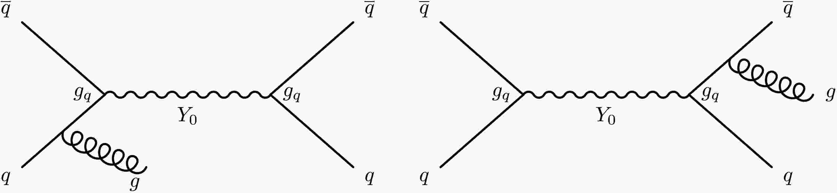
$Y_0 $ , in a simplified dark matter model [12−14]. If a heavy particle can be produced at a hadron collider, it should have sizeable couplings to quarks, which consequently gives a large enough branching ratio to di-jet final states. The di-jet search is a natural strategy to look for such a heavy particle and test those relevant BSM theories. As long as there is a new particle coupled to quarks or gluons with a narrow decay width, the di-jet search retains its power in any BSM models [15−17]. Many searches have been performed through various experiments, and the search strategy is rather well established, given its simple event topology. Those searches usually use the leading two jets, as they inherit most of the energy from the heavy particle decay. However, the events rarely contain only two jets, as there can be softer jets from initial-state radiation (ISR) and final-state radiation (FSR), as illustrated in Fig. 1. At the large hadron collider (LHC) experiments, such as ATLAS and CMS, there are also contributions from pile-up (PU) events. To overcome the trigger threshold constraints, experiments have also developed a search strategy that relies on an energetic ISR jet for the triggering so that the lower mass region below 1 TeV can be probed without significant biases [18, 19]. In this case, the leading two jets are not necessarily associated with the new particle. This work is concentrated on the mass region above 1 TeV, where the invariant mass of the leading two jets,$ m_{jj}$ , corresponds to the reconstructed heavy particle mass.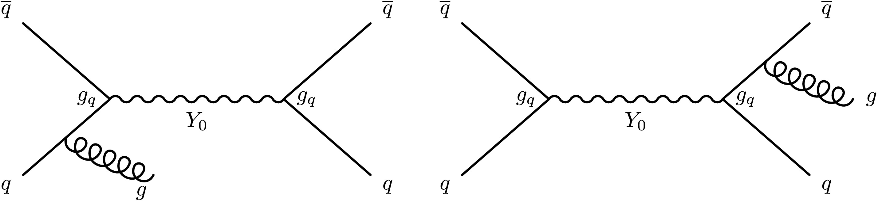
Although
$m_{jj}$ formed by the leading two jets has been proven to be effective, it is important to thoroughly investigate the impact from the FSR. In principle, the FSR jets should be included in the invariant mass calculation to better reconstruct the heavy particle mass. To do so, one must identify FSR jets while rejecting other softer jets in the events. Jets from PU are usually dealt with by experiments using dedicated techniques [20], so this study does not consider those jets.Some previous publications have proposed the use of ISR tagging and constructed a few observables [21]. It has also been discussed how the ISR jets affect the new physics processes [22−25]. More recently, a study explored a machine-learning-based (ML-based) technique to classify the nature of heavy particles with the aid from the soft jets [26]. However, the impact on the background and overall analysis were not examined extensively. It is of more importance at the current stage of the BSM search programs at the LHC to enhance sensitivity rather than distinguish the nature of new physics. In this study, we develop an FSR jet tagging algorithm using an ML-based approach that accounts for both the signal and background. This algorithm is constructed using basic kinematic variables of the jets, not sensitive to details of the parton showering setups. Meanwhile, the training procedure is designed to minimize
$ m_{jj}$ dependence such that it can be applied in di-jet searches using well established strategies. We show that the mass resolution of the signal, as well as the search sensitivity, can be greatly improved. In the light of high-luminosity LHC (HL-LHC), where the integrated luminosity is expected to exceed 3000 fb−1, the search program may go through different phases. In the beginning, attention shall be paid to the discovery potential, while the signal mass resolution may play a more critical role later on after an excess is found. The established method is capable of adopting those scenarios owing to its flexibility. This work identifies a promising avenue to enhance di-jet like resonance searches systematically, and the findings may be valuable for other hadronic searches as well.The remainder of this article is structured as follows. The datasets are introduced in Section II, followed by a study on the kinematic properties in Section III. The algorithm is detailed in Section IV, and Section V discusses its applications. Finally, Section VI summarizes the study and offers some thoughts for future work.
-
The search for a heavy particle decaying to two jets, i.e., the di-jet search, has a long history in collider experiments [1−8]. It is sensitive to a broad range of beyond the standard model (BSM) theories. The heavy particle can be the mediator connecting the standard model (SM) and BSM sectors [9−11], such as the spin-0 mediator,
$Y_0 $ , in a simplified dark matter model [12−14]. If a heavy particle can be produced at a hadron collider, it ought to have sizeable couplings to quarks, which consequently gives a large enough branching ratio to di-jet final states. The di-jet search is a natural strategy to look for such a heavy particle, and test those relevant BSM theories. As long as there is a new particle coupled to quarks or gluons, with a narrow decay width, the di-jet search retains its power to any BSM models [15−17]. Many searches have been performed in various experiments, and the search strategy is rather well established, given its simple event topology. Those searches usually use the leading two jets, as they inherit most of the energy from the heavy particle decay. However, the events rarely contain only two jets, as there can be softer jets from initial-state radiation (ISR) and final-state radiation (FSR), as illustrated in Figure 1. At the large hadron collider (LHC) experiments, such as ATLAS and CMS, there are also contributions from pile-up (PU) events. To overcome the trigger threshold constraints, experiments have also developed a search strategy that relies on an energetic ISR jet for the triggering so that the lower mass region below 1 TeV can be probed without significant biases [18, 19]. In this case, the leading two jets are not necessarily associated with the new particle. This work is concentrated on the mass region above 1 TeV, where the invariant mass of the leading two jets,$ m_{{\rm{jj}}}$ , corresponds to the reconstructed heavy particle mass.
Although
$ m_{{\rm{jj}}}$ formed by the leading two jets has been proven to be effective, it is important to thoroughly investigate the impact from the FSR. In principle, the FSR jets should be included in the invariant mass calculation to better reconstruct the heavy particle mass. To do so, one needs a way to identify FSR jets while rejecting other softer jets in the events. Jets from PU are usually dealt with by the experiments using dedicated techniques [20], so this study does not consider those jets.Some previous publications have proposed the usage of ISR tagging, and constructed a few observables [21]. It has also been discussed how the ISR jets affect the new physics processes [22−25]. More recently, a study explored a machine-learning-based (ML-based) technique to classify the nature of heavy particles with the aid from the soft jets [26]. However, the impact on the background and the overall analysis is not examined extensively. It is of more importance at the current stage of the BSM search programmes at the LHC to enhance the sensitivity, than to distinguish the nature of new physics. In this article, we develop an FSR jet tagging algorithm using a ML-based approach that accounts for both the signal and background. This algorithm is constructed using basic kinematic variables of the jets, not sensitive to details of the parton showering setups. Meanwhile, the training procedure is designed to minimise
$ m_{{\rm{jj}}}$ dependence so that it can be applied in di-jet searches using well established strategies. We show that the mass resolution of the signal can be greatly improved, as well as the search sensitivity. In the light of high-luminosity LHC (HL-LHC), where the integrated luminosity is expected to exceed 3000 fb−1, the search programme may go through different phases. In the beginning, attention shall be paid to the discovery potential, while later the signal mass resolution may play a more critical role after an excess is found. The method established is capable of adopting those scenarios, owing to its flexibility. This work identifies a promising avenue to enhance the di-jet like resonance searches systematically, and the findings may be valuable for other hadronic searches as well.The article is structured as follows, the datasets are introduced in Section 2, followed by a study on the kinematic properties in Section 3; the algorithm is detailed in Section 4, and Section 5 discusses its applications; finally Section 6 summarises the studies and offers some thoughts for future work.
-
The search for a heavy particle decaying into two jets, i.e., the di-jet search, has a long history in collider experiments [1−8]. It is sensitive to a broad range of beyond the standard model (BSM) theories. The heavy particle can be the mediator connecting the standard model (SM) and BSM sectors [9−11], such as the spin-0 mediator,
$Y_0 $ , in a simplified dark matter model [12−14]. If a heavy particle can be produced at a hadron collider, it should have sizeable couplings to quarks, which consequently gives a large enough branching ratio to di-jet final states. The di-jet search is a natural strategy to look for such a heavy particle and test those relevant BSM theories. As long as there is a new particle coupled to quarks or gluons with a narrow decay width, the di-jet search retains its power in any BSM models [15−17]. Many searches have been performed through various experiments, and the search strategy is rather well established, given its simple event topology. Those searches usually use the leading two jets, as they inherit most of the energy from the heavy particle decay. However, the events rarely contain only two jets, as there can be softer jets from initial-state radiation (ISR) and final-state radiation (FSR), as illustrated in Fig. 1. At the large hadron collider (LHC) experiments, such as ATLAS and CMS, there are also contributions from pile-up (PU) events. To overcome the trigger threshold constraints, experiments have also developed a search strategy that relies on an energetic ISR jet for the triggering so that the lower mass region below 1 TeV can be probed without significant biases [18, 19]. In this case, the leading two jets are not necessarily associated with the new particle. This work is concentrated on the mass region above 1 TeV, where the invariant mass of the leading two jets,$ m_{jj}$ , corresponds to the reconstructed heavy particle mass.
Although
$m_{jj}$ formed by the leading two jets has been proven to be effective, it is important to thoroughly investigate the impact from the FSR. In principle, the FSR jets should be included in the invariant mass calculation to better reconstruct the heavy particle mass. To do so, one must identify FSR jets while rejecting other softer jets in the events. Jets from PU are usually dealt with by experiments using dedicated techniques [20], so this study does not consider those jets.Some previous publications have proposed the use of ISR tagging and constructed a few observables [21]. It has also been discussed how the ISR jets affect the new physics processes [22−25]. More recently, a study explored a machine-learning-based (ML-based) technique to classify the nature of heavy particles with the aid from the soft jets [26]. However, the impact on the background and overall analysis were not examined extensively. It is of more importance at the current stage of the BSM search programs at the LHC to enhance sensitivity rather than distinguish the nature of new physics. In this study, we develop an FSR jet tagging algorithm using an ML-based approach that accounts for both the signal and background. This algorithm is constructed using basic kinematic variables of the jets, not sensitive to details of the parton showering setups. Meanwhile, the training procedure is designed to minimize
$ m_{jj}$ dependence such that it can be applied in di-jet searches using well established strategies. We show that the mass resolution of the signal, as well as the search sensitivity, can be greatly improved. In the light of high-luminosity LHC (HL-LHC), where the integrated luminosity is expected to exceed 3000 fb−1, the search program may go through different phases. In the beginning, attention shall be paid to the discovery potential, while the signal mass resolution may play a more critical role later on after an excess is found. The established method is capable of adopting those scenarios owing to its flexibility. This work identifies a promising avenue to enhance di-jet like resonance searches systematically, and the findings may be valuable for other hadronic searches as well.The remainder of this article is structured as follows. The datasets are introduced in Section II, followed by a study on the kinematic properties in Section III. The algorithm is detailed in Section IV, and Section V discusses its applications. Finally, Section VI summarizes the study and offers some thoughts for future work.
-
All samples used in this work are generated using MᴀᴅGʀᴀᴘʜ5_aMC@NLO 2.9.18 [27], showered by Pʏᴛʜɪᴀ 8.306 [28], and reconstructed in Delphes 3.5.3 [29]. The CMS detector geometry and performance are used for reconstruction, and the jets are clustered with a radius of
$ R = 0.4 $ , using the anti-$ k_t $ [30, 31] algorithm.Only the leading order process, with no additional partons, is generated with MᴀᴅGʀᴀᴘʜ5_aMC@NLO, so the FSR and ISR jets are only from the parton showering step done in Pʏᴛʜɪᴀ. Three scenarios are considered based on the "PartonLevel:ISR" and "PartonLevel:FSR" switches [32]. The nominal samples are showered with both switches on. Samples with either of the two turned off are prepared to gain insights on the input variables and validate the ISR jet labelling as discussed in Section 4.1, referred to as the showering control samples. Table 1 summarises those configurations.
Type PartonLevel:ISR PartonLevel:FSR nominal on on fsr control off on isr control on off Table 1. Summary of the showering configurations used to produce the samples.
-
All samples used in this work were generated using MᴀᴅGʀᴀᴘʜ5_aMC@NLO 2.9.18 [27], showered by Pʏᴛʜɪᴀ 8.306 [28], and reconstructed in Delphes 3.5.3 [29]. The CMS detector geometry and performance are used for reconstruction, and the jets are clustered with a radius of
$ R = 0.4 $ , using the anti-$ k_t $ [30, 31] algorithm.Only the leading order process, with no additional partons, is generated with MᴀᴅGʀᴀᴘʜ5_aMC@NLO, so the FSR and ISR jets are only from the parton showering step done in Pʏᴛʜɪᴀ. Three scenarios are considered based on the "PartonLevel:ISR" and "PartonLevel:FSR" switches [32]. The nominal samples are showered with both switches on. Samples with either of the two turned off are prepared to gain insights on the input variables and validate the ISR jet labeling, as discussed in Section IV.A, referred to as the showering control samples. Table 1 summarizes those configurations.
Type PartonLevel:ISR PartonLevel:FSR nominal on on fsr control off on isr control on off Table 1. Summary of the showering configurations used to produce the samples.
-
All samples used in this work were generated using MᴀᴅGʀᴀᴘʜ5_aMC@NLO 2.9.18 [27], showered by Pʏᴛʜɪᴀ 8.306 [28], and reconstructed in Delphes 3.5.3 [29]. The CMS detector geometry and performance are used for reconstruction, and the jets are clustered with a radius of
$ R = 0.4 $ , using the anti-$ k_t $ [30, 31] algorithm.Only the leading order process, with no additional partons, is generated with MᴀᴅGʀᴀᴘʜ5_aMC@NLO, so the FSR and ISR jets are only from the parton showering step done in Pʏᴛʜɪᴀ. Three scenarios are considered based on the "PartonLevel:ISR" and "PartonLevel:FSR" switches [32]. The nominal samples are showered with both switches on. Samples with either of the two turned off are prepared to gain insights on the input variables and validate the ISR jet labeling, as discussed in Section 4.1, referred to as the showering control samples. Table 1 summarizes those configurations.
Type PartonLevel:ISR PartonLevel:FSR nominal on on fsr control off on isr control on off Table 1. Summary of the showering configurations used to produce the samples.
-
The benchmark signal is a simplified dark matter model with a spin-0 mediator, Y0 [12−14]. It has equal couplings to all types of quarks, but the decay to a top-quark pair is not included. Model parameters are not modified to take the recent theoretical advances or experimental constraints into account, as the main kinematic characteristics of the model are not affected much by those. Five
$m_{Y_0} $ points are produced for the training steps, iterating from 1000 GeV to 3000 GeV with a step size of 500 GeV. Each point consists of 250 K events. Four additional points are produced to test the generality of the algorithm, from 3500 GeV to 5000 GeV in steps of 500 GeV. -
The benchmark signal is a simplified dark matter model with a spin-0 mediator, Y0 [12−14]. It has equal couplings to all types of quarks, but the decay to a top-quark pair is not included. Model parameters are not modified to take the recent theoretical advances or experimental constraints into account, as the main kinematic characteristics of the model are not affected much by those. Five
$m_{Y_0} $ points are produced for the training step, starting from 1000 GeV to 3000 GeV, with a step of 500 GeV. Each point consists of 250 K events. Four additional points are produced to test the generality of the algorithm, starting from 3500 GeV to 5000 GeV, with a step of 500 GeV. -
The benchmark signal is a simplified dark matter model with a spin-0 mediator, Y0 [12−14]. It has equal couplings to all types of quarks, but the decay to a top-quark pair is not included. Model parameters are not modified to take the recent theoretical advances or experimental constraints into account, as the main kinematic characteristics of the model are not affected much by those. Five
$m_{Y_0} $ points are produced for the training steps, iterating from 1000 GeV to 3000 GeV with a step size of 500 GeV. Each point consists of 250 K events. Four additional points are produced to test the generality of the algorithm, from 3500 GeV to 5000 GeV in steps of 500 GeV. -
The benchmark signal is a simplified dark matter model with a spin-0 mediator, Y0 [12−14]. It has equal couplings to all types of quarks, but the decay to a top-quark pair is not included. Model parameters are not modified to take the recent theoretical advances or experimental constraints into account, as the main kinematic characteristics of the model are not affected much by those. Five
$m_{Y_0} $ points are produced for the training steps, iterating from 1000 GeV to 3000 GeV with a step size of 500 GeV. Each point consists of 250 K events. Four additional points are produced to test the generality of the algorithm, from 3500 GeV to 5000 GeV in steps of 500 GeV. -
The major background in di-jet resonance searches is the SM QCD multi-jet production. As the training of the algorithm requires samples populated evenly in the entire phase space to avoid kinematic biases, three samples sliced by the leading jet
$p_{T}$ at the generation level are produced, with cuts 450 GeV, 900 GeV, and 1350 GeV. The lowest$p_{T}$ slice is motivated by the usual trigger criterion applied in inclusive di-jet analyses [5]. -
The major background in di-jet resonance searches is the SM QCD multi-jet production. As the training of the algorithm requires samples populated evenly in the entire phase space to avoid kinematic biases, three samples sliced by the leading jet
$p_{{\rm{T}}} $ at the generation level are produced, with a cut of 450 GeV, 900 GeV and 1350 GeV, respectively. The lowest$p_{{\rm{T}}} $ slice is motivated by the usual trigger criterion applied in the inclusive di-jet analyses [5]. -
A heavy resonance decaying into two quarks gives rise to two energetic jets. It is usually appropriate to assume that the leading two jets in
$p_{T}$ are from heavy particle decays, as long as the heavy particle mass is twice the threshold of the leading jet$p_{T}$ selection. Jets from FSR are strongly correlated with the leading two jets, while those from ISR are not. The showering control samples are used in this section to examine these correlations and motivate the design of the algorithm in Section IV.An energetic FSR jet can carry away a significant amount of energy from the heavy particle decay system, resulting in a smeared
$m_{jj}$ distribution. As shown in Fig. 2, once including the hardest FSR jet, the mass peak is already shifted closer to the actual$m_{Y_0} $ . Including additional softer FSR jets does bring further enhancements, but it is already sufficient to showcase the impact focusing on the hardest FSR jet. It is also evident from Fig. 2 that simply including softer jets in the mass calculation without checking whether they are from FSR or ISR is not a viable strategy. It introduces a sizeable high mass tail, making the peak much broader.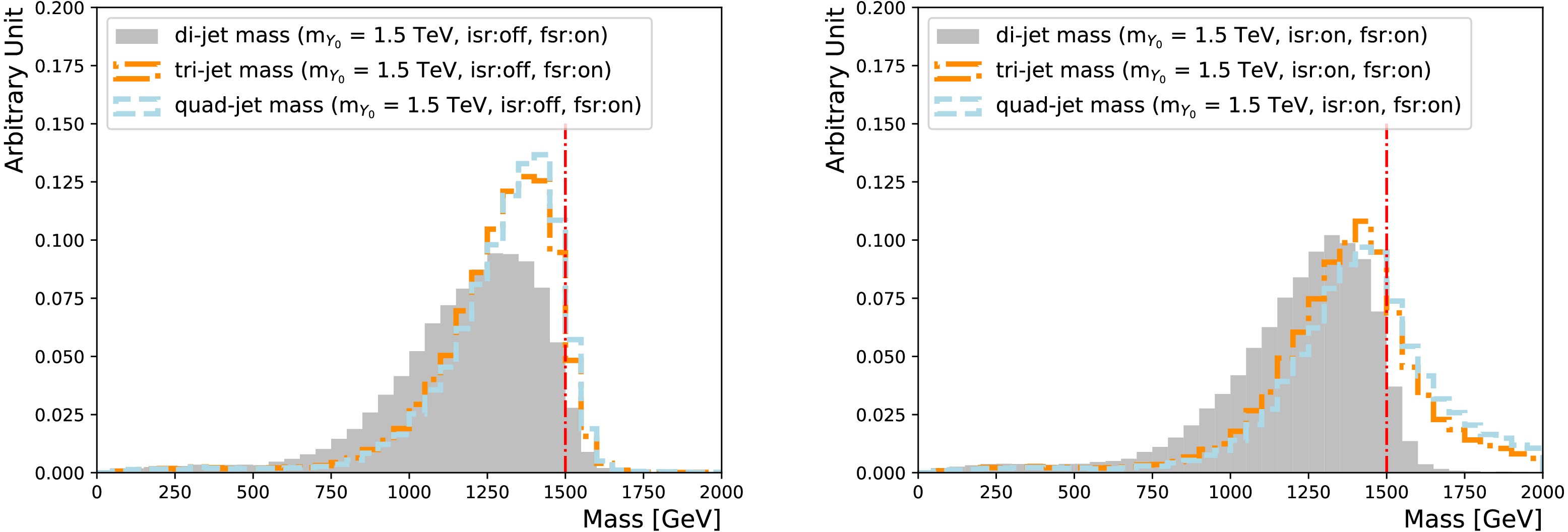
Figure 2. (color online) Comparison of the
$Y_0 $ mass reconstructed using the leading two jets (shaded area), leading three jets (dotted-dashed line), and leading four jets (dashed line), with the ISR showering switch turned off (left) and on (right). The FSR showering switch is turned on for both. The vertical line indicates the actual$Y_0 $ mass (1.5 TeV).The two leading jets from a heavy
$Y_0 $ particle, produced via the s-channel, are central and back-to-back. Because the hardest FSR jet is branched from those two leading jets, it should be close to one of them spatially, resulting in central η and peaks in$\Delta\phi $ with respect to the leading two jets. The kinematic properties of the ISR jets rely on the incoming partons, so their corresponding distributions are wider. Figure 3 compares the key variables of FSR jets to those of ISR jets using the showering control samples.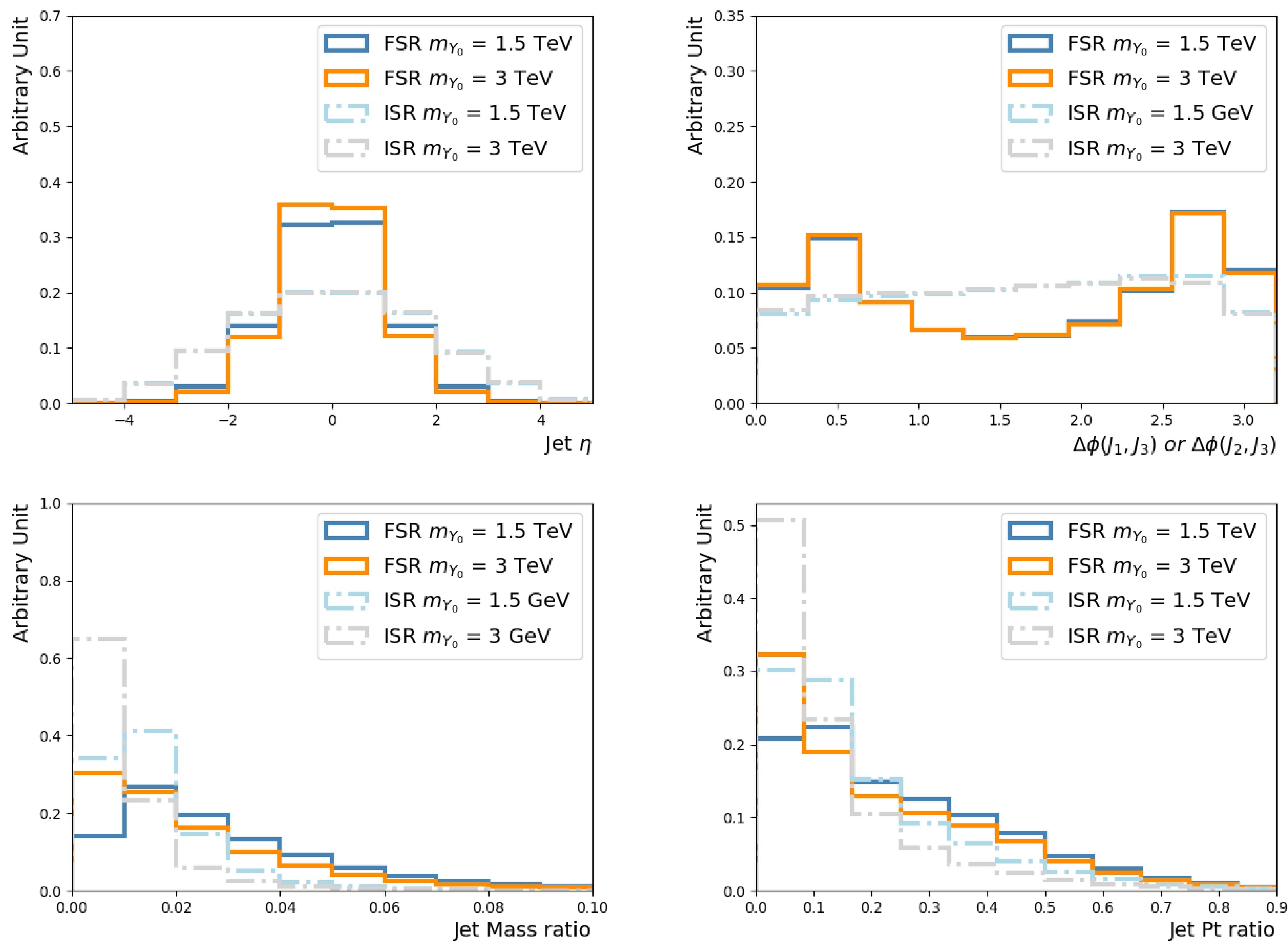
Figure 3. (color online) Selected kinematic distributions of the third jet for the
$m_{Y_0} $ = 1.5 TeV and 3 TeV samples. The third jets taken from the showering control samples with the FSR/ISR showering switch turned on/off and off/on are the FSR and ISR jets, respectively. Four quantities are shown: the third jet η (upper left),$ \Delta \phi $ between the third jet and (sub-)leading jet (upper right), and ratios of the third jet mass (lower left) and$p_{T}$ (lower right) to the leading jet$p_{T}$ .The above observations for the signal processes still hold largely for the QCD multi-jet, as the underlying showering process is the same, as shown in Fig. 4. However, high
$m_{jj}$ QCD multi-jet events are dominated by t-channel production, and the leading two jets are more likely to originate from gluons compared to the signal. These differences allow the algorithm to distinguish FSR jets in the signal from those in the background.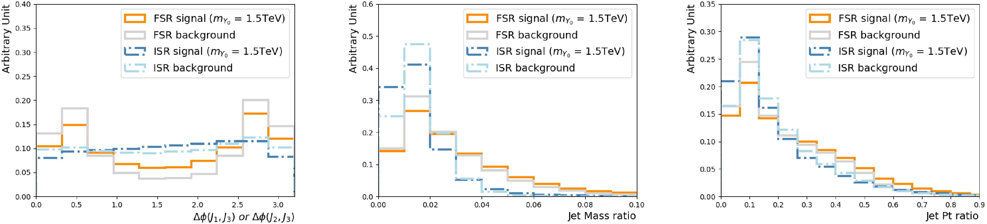
Figure 4. (color online) Selected kinematic distributions of the third jet for the
$m_{Y_0} $ = 1.5 TeV signal and multi-jet background. The third jets taken from the showering control samples with the FSR/ISR showering switch turned on/off and off/on, are the FSR and ISR jets, respectively. Three quantities are shown:$ \Delta \phi $ between the third jet and the (sub-)leading jet (left), ratio of the third jet mass (middle) and$p_{T} $ (right) to the leading jet$p_{T} $ .It is already known that using charged particles within the jets allows us to distinguish gluon-initiated jets from quark-initiated jets [33]. The colour connections between the radiated partons and the outgoing partons will also impact the jet constituents [22, 34, 35]. Adding lower-level input features can further enhance the performance. However, doing so makes the algorithm subject to the detailed parton shower setups and detector resolutions. This should be studied with great care, and we leave it for future works.
-
A heavy resonance decaying to two quarks gives rise to two energetic jets. It is usually appropriate to assume that the leading two jets in
$p_{{\rm{T}}} $ are from heavy particle decays, as long as the heavy particle mass is twice the threshold of the leading jet$p_{{\rm{T}}} $ selection. Jets from FSR are strongly correlated with the leading two jets, while those from ISR are not. The showering control samples are used in this section to examine these correlations and motivate the design of the algorithm in Section 4.An energetic FSR jet can carry away a significant amount of energy from the heavy particle decay system, resulting in a smeared
$ m_{{\rm{jj}}}$ distribution. As seen in Figure 2, once including the hardest FSR jet, the mass peak is already shifted closer to the actual$m_{Y_0} $ . Including additional softer FSR jets does bring further enhancements, but it is already sufficient to showcase the impact focusing on the hardest FSR jet. It is also obvious in Figure 2 that simply including softer jets in the mass calculation, without checking whether they are from FSR or ISR, is not a viable strategy. It introduces a sizeable high mass tail, making the peak much broader.
Figure 2. (color online) Comparison of the
$Y_0 $ mass reconstructed using the leading two jets (shaded area), the leading three jets (dotted-dashed line) and the leading four jets (dashed line), with the ISR showering switch turned off (left) and on (right). The FSR showering switch is turned on for both. The vertical line indicates the actual$Y_0 $ mass (1.5 TeV).The two leading jets from a heavy
$Y_0 $ particle, produced via s-channel, are central and back-to-back. Since the hardest FSR jet is branched from those two leading jets, it should be close to one of them spacially, resulting in central η and peaks in$\Delta\phi $ w.r.t the leading two jets. The kinematic properties of the ISR jets rely on the incoming partons, so their corresponding distributions are wider. Figure 3 compares the key variables of FSR jets to those of ISR jets, using the showering control samples.
Figure 3. (color online) Selected kinematic distributions of the third jet for the
$m_{Y_0} $ = 1.5 TeV and 3 TeV samples. The third jets taken from the showering control samples with the FSR/ISR showering switch turned on/off and off/on, are the FSR and ISR jets, respectively. Four quantities are shown: the third jet η (upper left),$ \Delta \phi $ between the third jet and the (sub-)leading jet (upper right), ratio of the third jet mass (lower left) and$p_{{\rm{T}}} $ (lower right) to the leading jet$p_{{\rm{T}}} $ .The above observations for the signal processes still hold largely for the QCD multi-jet, as the underlying showering process is the same, as seen in Figure 4. However, high
$ m_{{\rm{jj}}}$ QCD multi-jet events are dominated by the t-channel production, and the leading two jets are more likely to originate from gluons, compared to the signal. Those differences allow the algorithm to distinguish FSR jets in signal from those in background.
Figure 4. (color online) Selected kinematic distributions of the third jet for the
$m_{Y_0} $ = 1.5 TeV signal and multi-jet background. The third jets taken from the showering control samples with the FSR/ISR showering switch turned on/off and off/on, are the FSR and ISR jets, respectively. Three quantities are shown:$ \Delta \phi $ between the third jet and the (sub-)leading jet (left), ratio of the third jet mass (middle) and$p_{{\rm{T}}} $ (right) to the leading jet$p_{{\rm{T}}} $ .It is already seen that using charged particles within the jets allows us to distinguish gluon-initiated jets from quark-initiated jets [33]. The colour connections between the radiated partons and the outgoing partons will also impact the jet constituents [22, 34, 35]. Adding lower level input features can further enhance the performance. However, doing so makes the algorithm subject to the detailed parton shower setups and detector resolutions. It should be studied with great care, and we leave it for future works.
-
A heavy resonance decaying into two quarks gives rise to two energetic jets. It is usually appropriate to assume that the leading two jets in
$p_{T}$ are from heavy particle decays, as long as the heavy particle mass is twice the threshold of the leading jet$p_{T}$ selection. Jets from FSR are strongly correlated with the leading two jets, while those from ISR are not. The showering control samples are used in this section to examine these correlations and motivate the design of the algorithm in Section IV.An energetic FSR jet can carry away a significant amount of energy from the heavy particle decay system, resulting in a smeared
$m_{jj}$ distribution. As shown in Fig. 2, once including the hardest FSR jet, the mass peak is already shifted closer to the actual$m_{Y_0} $ . Including additional softer FSR jets does bring further enhancements, but it is already sufficient to showcase the impact focusing on the hardest FSR jet. It is also evident from Fig. 2 that simply including softer jets in the mass calculation without checking whether they are from FSR or ISR is not a viable strategy. It introduces a sizeable high mass tail, making the peak much broader.
Figure 2. (color online) Comparison of the
$Y_0 $ mass reconstructed using the leading two jets (shaded area), leading three jets (dotted-dashed line), and leading four jets (dashed line), with the ISR showering switch turned off (left) and on (right). The FSR showering switch is turned on for both. The vertical line indicates the actual$Y_0 $ mass (1.5 TeV).The two leading jets from a heavy
$Y_0 $ particle, produced via the s-channel, are central and back-to-back. Because the hardest FSR jet is branched from those two leading jets, it should be close to one of them spatially, resulting in central η and peaks in$\Delta\phi $ with respect to the leading two jets. The kinematic properties of the ISR jets rely on the incoming partons, so their corresponding distributions are wider. Figure 3 compares the key variables of FSR jets to those of ISR jets using the showering control samples.
Figure 3. (color online) Selected kinematic distributions of the third jet for the
$m_{Y_0} $ = 1.5 TeV and 3 TeV samples. The third jets taken from the showering control samples with the FSR/ISR showering switch turned on/off and off/on are the FSR and ISR jets, respectively. Four quantities are shown: the third jet η (upper left),$ \Delta \phi $ between the third jet and (sub-)leading jet (upper right), and ratios of the third jet mass (lower left) and$p_{T}$ (lower right) to the leading jet$p_{T}$ .The above observations for the signal processes still hold largely for the QCD multi-jet, as the underlying showering process is the same, as shown in Fig. 4. However, high
$m_{jj}$ QCD multi-jet events are dominated by t-channel production, and the leading two jets are more likely to originate from gluons compared to the signal. These differences allow the algorithm to distinguish FSR jets in the signal from those in the background.
Figure 4. (color online) Selected kinematic distributions of the third jet for the
$m_{Y_0} $ = 1.5 TeV signal and multi-jet background. The third jets taken from the showering control samples with the FSR/ISR showering switch turned on/off and off/on, are the FSR and ISR jets, respectively. Three quantities are shown:$ \Delta \phi $ between the third jet and the (sub-)leading jet (left), ratio of the third jet mass (middle) and$p_{T} $ (right) to the leading jet$p_{T} $ .It is already known that using charged particles within the jets allows us to distinguish gluon-initiated jets from quark-initiated jets [33]. The colour connections between the radiated partons and the outgoing partons will also impact the jet constituents [22, 34, 35]. Adding lower-level input features can further enhance the performance. However, doing so makes the algorithm subject to the detailed parton shower setups and detector resolutions. This should be studied with great care, and we leave it for future works.
-
The di-jet resonance search usually adopts a data-driven approach to estimate the background. A classic method is to apply a functional fit to
$ m_{{\rm{jj}}}$ in data [1−8]. There are several new strategies proposed such as Gaussian Process Regression [36−39], symbolic regression [40] and orthonormal series [41]. All these methods assume the background$ m_{{\rm{jj}}}$ is smooth, so significant sculpting of the$ m_{{\rm{jj}}}$ will challenge the analysis methodology. Furthermore, the di-jet searches often try to probe a wide$ m_{{\rm{jj}}}$ range without assuming the mass of the hypothetical heavy particle. As a result, the algorithm should introduce as minimal$ m_{{\rm{jj}}}$ dependence as possible. Variables strongly correlated with$ m_{{\rm{jj}}}$ , such as the jet$p_{{\rm{T}}} $ and mass, are not directly used in the training. As seen in Figure 3 and Figure 4, dimensionless ratios calculated using those variables, w.r.t the leading jet$p_{{\rm{T}}} $ , hold separation power. Those ratios are used in the training, which also makes all the input features at a similar magnitude. Data scaling or normalisation is found to have very minimal impact so that it is not imposed.Given the overwhelming multi-jet background, it is imperative to consider the algorithm's performance there as well. If the FSR jets in the background are tagged, the background
$ m_{{\rm{jj}}}$ is shifted towards higher values, which may cancel the improvements brought to the signal$ m_{{\rm{jj}}}$ resolution. Therefore, the algorithm is designed and trained to classify four categories: "sig-isr", "sig-fsr", "bkg-isr" and "bkg-fsr", corresponding to ISR/FSR jets in the signal/background events. The procedure to label the ISR jets is described in the next section. -
The di-jet resonance search usually adopts a data-driven approach to estimate the background. A classic method is to apply a functional fit to
$ m_{jj}$ in data [1−8]. Several new strategies have been proposed, such as Gaussian Process Regression [36−39], symbolic regression [40], and orthonormal series [41]. All these methods assume the background$ m_{jj}$ is smooth, so significant sculpting of the$ m_{jj}$ will challenge the analysis methodology. Furthermore, di-jet searches often try to probe a wide$ m_{jj}$ range without assuming the mass of the hypothetical heavy particle. As a result, the algorithm should introduce as minimal$ m_{jj}$ dependence as possible. Variables strongly correlated with$ m_{jj}$ , such as the jet$p_{T} $ and mass, are not directly used in the training. As shown in Fig. 3 and Fig. 4, dimensionless ratios calculated using those variables, with respect to the leading jet$p_{T} $ , hold separation power. Those ratios are used in the training, which also makes all the input features have a similar magnitude. Data scaling or normalization is found to have very minimal impact, so it is not imposed.Given the overwhelming multi-jet background, it is imperative to consider the algorithm's performance there as well. If the FSR jets in the background are tagged, the background
$ m_{jj}$ is shifted towards higher values, which may cancel the improvements brought to the signal$ m_{jj}$ resolution. Therefore, the algorithm is designed and trained to classify four categories: "sig-isr," "sig-fsr," "bkg-isr," and "bkg-fsr," corresponding to ISR/FSR jets in the signal/background events. The procedure to label the ISR jets is described in the next section. -
Particles initialized by the ISR or FSR processes can be identified by the Pʏᴛʜɪᴀᴠ status code. A status code between 41 (51) and 49 (59) means the corresponding particle is from ISR (FSR) [32]. Those particles are matched to a given jet by a cone with
$ \Delta R \lt 0.4 $ , allowing us to determine whether it is an ISR or FSR jet. To minimize the effects from soft emissions, only particles with$p_{T} $ > 0.5 GeV are included. However, as shown in Fig. 5, the third jet in the event usually has both ISR and FSR particles associated.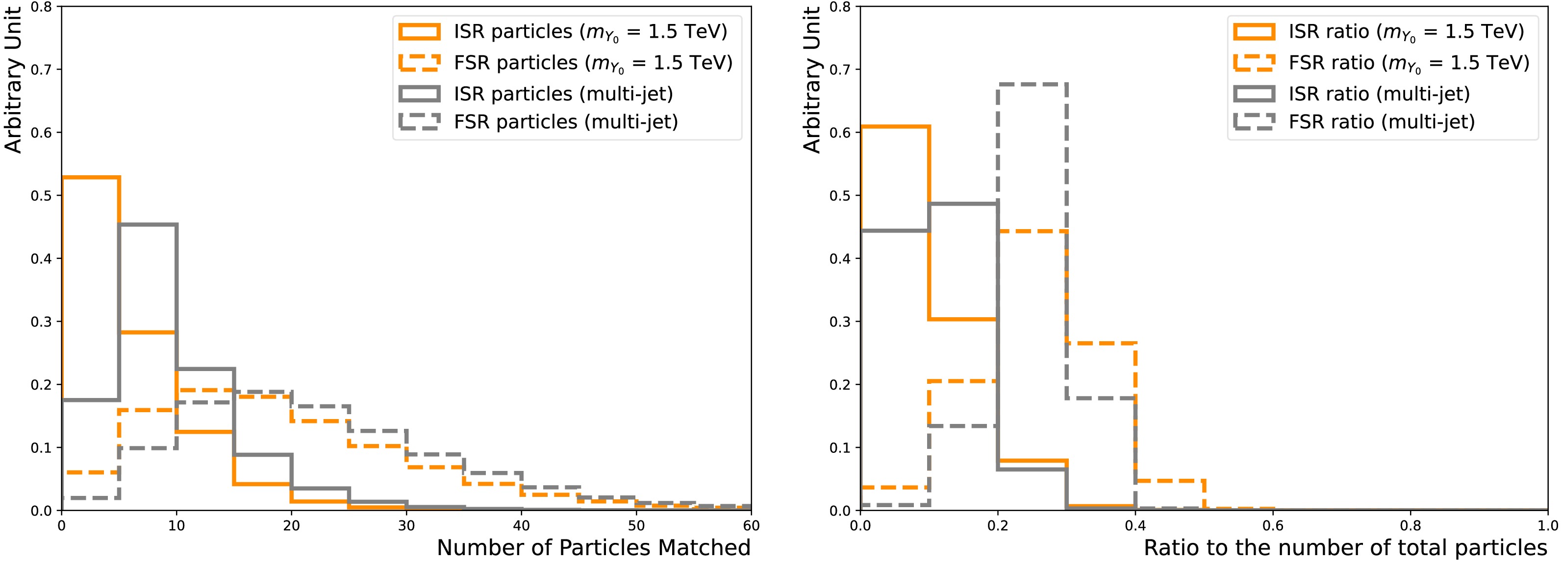
Figure 5. (color online) Numbers of FSR particles (dotted-dashed line) and ISR particles (solid line) associated with the third jet (left). RatioS of the number of FSR particles (dotted-dashed line) and ISR particles (solid line) to the total number of particles, including those not from ISR/FSR, associated with the third jet (right). The nominal
$m_{Y_0} $ = 1.5 TeV signal (dark orange) and multi-jet background (light gray) samples are used.The scalar summation of the
$p_{T} $ ,$\Sigma p_{T} $ , can better reflect the origin of the jets. The ratio between$\Sigma p_{T} $ of the ISR particles to that of the FSR particles, illustrated in Fig. 6, is used for ISR jet labeling. Jets with this ratio above one are taken as ISR jets. Figure 7 compares the η distributions of the third jet obtained via this ISR labeling method and those in the showering control samples, where reasonable agreements are observed. The$m_{Y_0} $ = 1500 GeV signal is used as an example in this section, and we observe similar behaviors for other masses as well.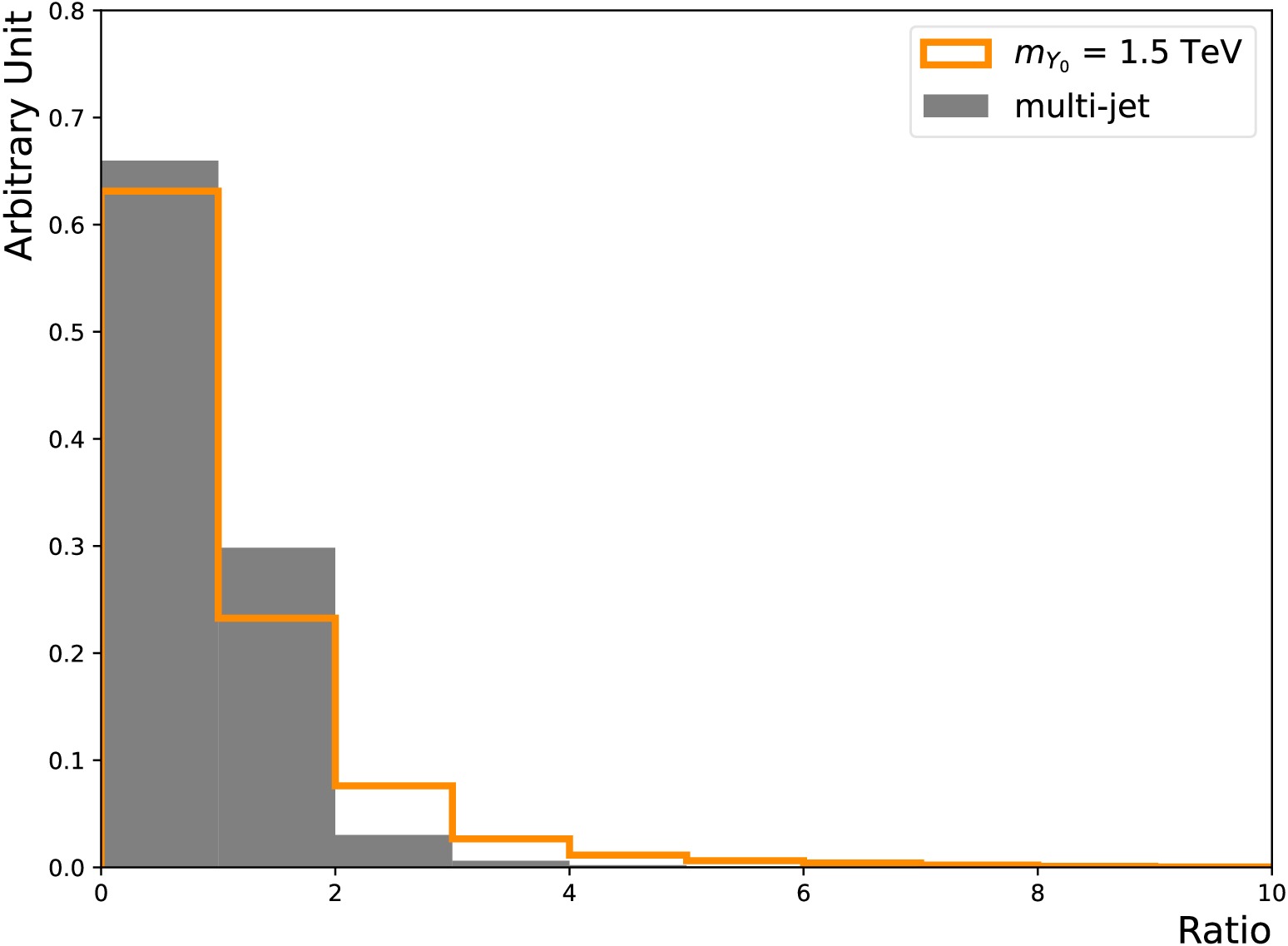
Figure 6. (color online) Ratios between the scalar sum of associated ISR particle
$p_{T} $ to that of associated FSR particle$p_{T} $ for the third jet in the$m_{Y_0} $ = 1.5 TeV signal (solid line) and multi-jet background (shaded area) nominal samples.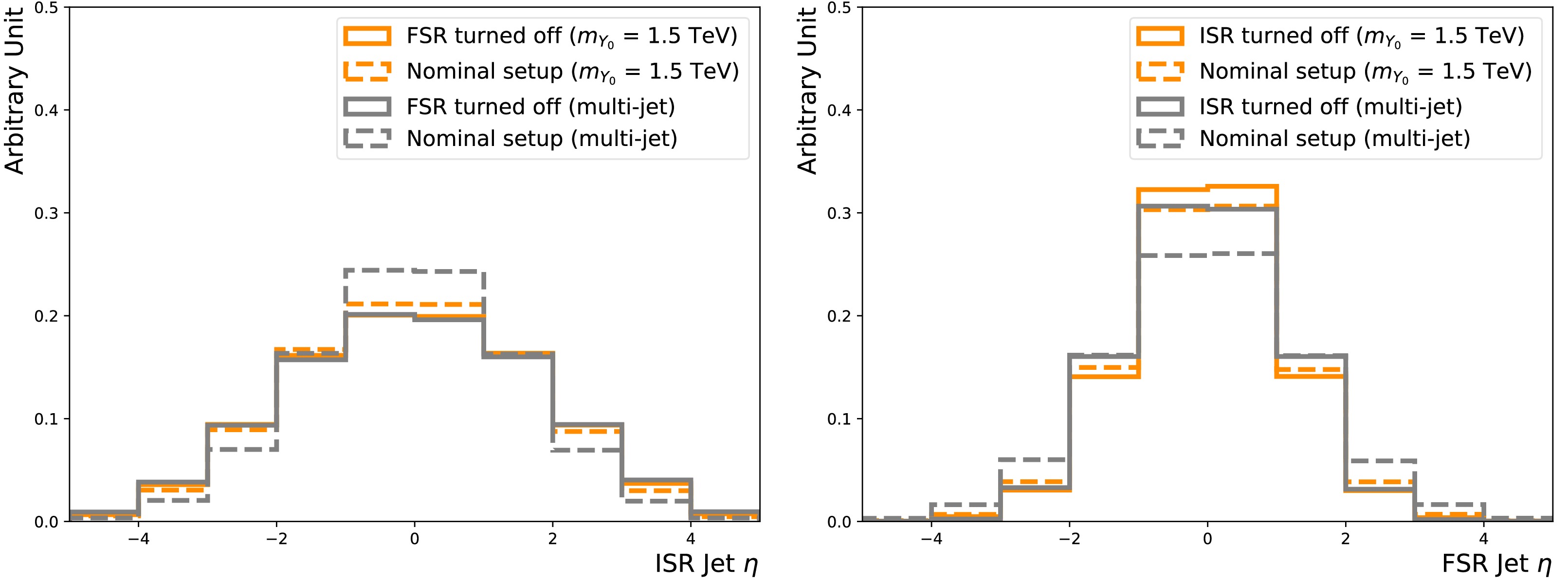
Figure 7. (color online) Comparison of the ISR jet (left) and FSR jet (right) η (left) between those in the nominal sample labeled by the above criterion (dotted-dashed line) and those in the corresponding showering control sample (solid line). The
$m_{Y_0} $ = 1.5 TeV signal (dark orange) and multi-jet background (light gray) are shown. -
Particles initialised by the ISR or FSR processes can be identified by the Pʏᴛʜɪᴀᴠ status code. A status code between 41 (51) and 49 (59) means the corresponding particle is from ISR (FSR) [32]. Those particles are matched to a given jet by a cone with
$ \Delta R < 0.4 $ , allowing us to determine whether it is an ISR or FSR jet. Only particles with$p_{{\rm{T}}} $ > 0.5 GeV are included, to minimise the effects from soft emissions. However, as seen in Figure 5, the third jet in the event usually has both ISR and FSR particles associated.
Figure 5. (color online) The number of FSR particles (dotted-dashed line) and ISR particles (solid line) associated with the third jet (left). The ratio of the number of FSR particles (dotted-dashed line) and ISR particles (solid line) to the total number of particles, including those not from ISR/FSR, associated with the third jet (right). The nominal
$m_{Y_0} $ = 1.5 TeV signal (dark orange) and multi-jet background (light grey) samples are used.The scalar summation of the
$p_{{\rm{T}}} $ ,$\Sigma p_{{\rm{T}}} $ , can better reflect the origin of the jets. The ratio between$\Sigma p_{{\rm{T}}} $ of the ISR particles to that of the FSR particles, illustrated in Figure 6, is used for ISR jet labelling. Jets with this ratio above one are taken as ISR jets. Figure 7 compares the η distributions of the third jet obtained via this ISR labelling method and those in the showering control samples, where reasonable agreements are observed. The$m_{Y_0} $ = 1500 GeV signal is used as an example in this section, and we observe similar behaviours for other masses as well.
Figure 6. (color online) Ratio between the scalar sum of associated ISR particle
$p_{{\rm{T}}} $ , to that of associated FSR particle$p_{{\rm{T}}} $ , for the third jet in the$m_{Y_0} $ = 1.5 TeV signal (solid line) and multi-jet background (shaded area) nominal samples.
Figure 7. (color online) Comparison of the ISR jet (left) and FSR jet (right) η (left) between those in the nominal sample labelled by the above criterion (dotted-dashed line) and those in the corresponding showering control sample (solid line). The
$m_{Y_0} $ = 1.5 TeV signal (dark orange) and multi-jet background (light grey) are shown. -
Particles initialized by the ISR or FSR processes can be identified by the Pʏᴛʜɪᴀᴠ status code. A status code between 41 (51) and 49 (59) means the corresponding particle is from ISR (FSR) [32]. Those particles are matched to a given jet by a cone with
$ \Delta R \lt 0.4 $ , allowing us to determine whether it is an ISR or FSR jet. To minimize the effects from soft emissions, only particles with$p_{T} $ > 0.5 GeV are included. However, as shown in Fig. 5, the third jet in the event usually has both ISR and FSR particles associated.
Figure 5. (color online) Numbers of FSR particles (dotted-dashed line) and ISR particles (solid line) associated with the third jet (left). RatioS of the number of FSR particles (dotted-dashed line) and ISR particles (solid line) to the total number of particles, including those not from ISR/FSR, associated with the third jet (right). The nominal
$m_{Y_0} $ = 1.5 TeV signal (dark orange) and multi-jet background (light gray) samples are used.The scalar summation of the
$p_{T} $ ,$\Sigma p_{T} $ , can better reflect the origin of the jets. The ratio between$\Sigma p_{T} $ of the ISR particles to that of the FSR particles, illustrated in Fig. 6, is used for ISR jet labeling. Jets with this ratio above one are taken as ISR jets. Figure 7 compares the η distributions of the third jet obtained via this ISR labeling method and those in the showering control samples, where reasonable agreements are observed. The$m_{Y_0} $ = 1500 GeV signal is used as an example in this section, and we observe similar behaviors for other masses as well.
Figure 6. (color online) Ratios between the scalar sum of associated ISR particle
$p_{T} $ to that of associated FSR particle$p_{T} $ for the third jet in the$m_{Y_0} $ = 1.5 TeV signal (solid line) and multi-jet background (shaded area) nominal samples.
Figure 7. (color online) Comparison of the ISR jet (left) and FSR jet (right) η (left) between those in the nominal sample labeled by the above criterion (dotted-dashed line) and those in the corresponding showering control sample (solid line). The
$m_{Y_0} $ = 1.5 TeV signal (dark orange) and multi-jet background (light gray) are shown. -
The algorithm uses a simple feed-forward deep neural network, consisting of 12 input nodes, followed by four hidden layers, with 30, 60, 30, and 12 nodes, respectively. Each node has a ReLU activation applied [42]. A one-hot encoder is adopted to construct the target vector with four categories. Consequently, the network has four output nodes and uses a cross-entropy loss function.
The input features include η, ϕ, and the ratio between jet mass and jet
$p_{T} $ of the leading three jets, as well as the relative fractions of the jet momenta, as summarized in Table 2. The background is sampled from three$p_{T} $ sliced multi-jet samples, so the events are evenly distributed across leading jet$p_{T} $ . Five signal mass points, from 1000 GeV to 3000 GeV in increments of 500 GeV, are combined to populate the entire phase space. The leading jet$p_{T} $ is required to be within [450, 1750] GeV, and the dataset is sampled to have equal amounts of "bkg-isr" ("sig-isr") and "bkg-fsr" ("sig-fsr") events. The final dataset has approximately 420k background and 460k signal events.Type Features angular $ \eta^{{\rm{j}}_1} $ ,$ \eta^{{\rm{j}}_2} $ ,$ \eta^{{\rm{j}}_3} $ ,$ \phi^{{\rm{j}}_1} $ ,$ \phi^{{\rm{j}}_2} $ ,$ \phi^{{\rm{j}}_3} $ ratio $ m^{{\rm{j}}_1}/p_{T}^{{\rm{j}}_1} $ ,$ m^{{\rm{j}}_2}/p_{T}^{{\rm{j}}_2} $ ,$ m^{{\rm{j}}_3}/p_{T}^{{\rm{j}}_3} $ ,$ p_{T}^{{\rm{j}}_3}/p_{T}^{{\rm{j}}_1} $ ,$ p_{T}^{{\rm{j}}_3}/p_{T}^{{\rm{j}}_2} $ ,$ p_{T}^{{\rm{j}}_2}/p_{T}^{{\rm{j}}_1} $ Table 2. Summary of input features to train the classifier.
The training of the algorithm takes 80% of the dataset, with a batch size of 100. The SGD optimizer is employed [43], with a learning rate of 0.05. In total, 100 epochs are conducted, and the one with the best performance is selected.
-
The algorithm uses a simple feed-forward deep neural network, consisting of 12 input nodes, followed by four hidden layers, with 30, 60, 30 and 12 nodes, respectively. Each node has a ReLU activation applied [42]. A one-hot encoder is adopted to construct the target vector with four categories. Consequently, the network has four output nodes and uses a cross-entropy loss function.
The input features include η, ϕ and the ratio between jet mass and jet
$p_{{\rm{T}}} $ of the leading three jets, as well as the relative fractions of the jet momenta, summarised in Table 2. The background is sampled from three$p_{{\rm{T}}} $ sliced multi-jet samples, so the events are evenly distributed across leading jet$p_{{\rm{T}}} $ . Five signal mass points, starting from 1000 GeV to 3000 GeV, with a step of 500 GeV, are combined to populate the entire phase space. The leading jet$p_{{\rm{T}}} $ is required to be within [450, 1750] GeV, and the dataset is sampled to have an equal amount of "bkg-isr" ("sig-isr") and "bkg-fsr" ("sig-fsr") events. The final dataset has roughly 420k background and 460k signal events.Type Features angular $ \eta^{{\rm{j}}_1} $ ,$ \eta^{{\rm{j}}_2} $ ,$ \eta^{{\rm{j}}_3} $ ,$ \phi^{{\rm{j}}_1} $ ,$ \phi^{{\rm{j}}_2} $ ,$ \phi^{{\rm{j}}_3} $ ratio $ m^{{\rm{j}}_1}/p_{{\rm{T}}}^{{\rm{j}}_1} $ ,$ m^{{\rm{j}}_2}/p_{{\rm{T}}}^{{\rm{j}}_2} $ ,$ m^{{\rm{j}}_3}/p_{{\rm{T}}}^{{\rm{j}}_3} $ ,$ p_{{\rm{T}}}^{{\rm{j}}_3}/p_{{\rm{T}}}^{{\rm{j}}_1} $ ,$ p_{{\rm{T}}}^{{\rm{j}}_3}/p_{{\rm{T}}}^{{\rm{j}}_2} $ ,$ p_{{\rm{T}}}^{{\rm{j}}_2}/p_{{\rm{T}}}^{{\rm{j}}_1} $ Table 2. Summary of the input features to train the classifier
The training of the algorithm takes 80% of the dataset, with a batch size of 100. The SGD optimiser is employed [43], with a learning rate of 0.05. In total, 100 epochs are carried out and the one with the best performance is selected.
-
The algorithm uses a simple feed-forward deep neural network, consisting of 12 input nodes, followed by four hidden layers, with 30, 60, 30, and 12 nodes, respectively. Each node has a ReLU activation applied [42]. A one-hot encoder is adopted to construct the target vector with four categories. Consequently, the network has four output nodes and uses a cross-entropy loss function.
The input features include η, ϕ, and the ratio between jet mass and jet
$p_{T} $ of the leading three jets, as well as the relative fractions of the jet momenta, as summarized in Table 2. The background is sampled from three$p_{T} $ sliced multi-jet samples, so the events are evenly distributed across leading jet$p_{T} $ . Five signal mass points, from 1000 GeV to 3000 GeV in increments of 500 GeV, are combined to populate the entire phase space. The leading jet$p_{T} $ is required to be within [450, 1750] GeV, and the dataset is sampled to have equal amounts of "bkg-isr" ("sig-isr") and "bkg-fsr" ("sig-fsr") events. The final dataset has approximately 420k background and 460k signal events.Type Features angular $ \eta^{{\rm{j}}_1} $ ,$ \eta^{{\rm{j}}_2} $ ,$ \eta^{{\rm{j}}_3} $ ,$ \phi^{{\rm{j}}_1} $ ,$ \phi^{{\rm{j}}_2} $ ,$ \phi^{{\rm{j}}_3} $ ratio $ m^{{\rm{j}}_1}/p_{T}^{{\rm{j}}_1} $ ,$ m^{{\rm{j}}_2}/p_{T}^{{\rm{j}}_2} $ ,$ m^{{\rm{j}}_3}/p_{T}^{{\rm{j}}_3} $ ,$ p_{T}^{{\rm{j}}_3}/p_{T}^{{\rm{j}}_1} $ ,$ p_{T}^{{\rm{j}}_3}/p_{T}^{{\rm{j}}_2} $ ,$ p_{T}^{{\rm{j}}_2}/p_{T}^{{\rm{j}}_1} $ Table 2. Summary of input features to train the classifier.
The training of the algorithm takes 80% of the dataset, with a batch size of 100. The SGD optimizer is employed [43], with a learning rate of 0.05. In total, 100 epochs are conducted, and the one with the best performance is selected.
-
The neural network has four output nodes, corresponding to the probabilities for the third jet to be in the four categories "sig-isr," "sig-fsr," "bkg-isr," and "bkg-fsr." Therefore, they are denoted as
$ p_{{\rm{s}}}^{{\rm{i}}} $ ,$ p_{{\rm{s}}}^{{\rm{f}}} $ ,$ p_{{\rm{b}}}^{{\rm{i}}} $ , and$ p_{{\rm{b}}}^{{\rm{f}}} $ , respectively. A discriminating variable can be constructed to balance the target efficiency and false positive rates:$ D_{{\rm{s}}}^{{\rm{f}}} = \log \dfrac{p_{{\rm{s}}}^{{\rm{f}}}}{(f_{{\rm{s}}}^{{\rm{i}}} \cdot p_{{\rm{s}}}^{{\rm{i}}} + f_{{\rm{b}}}^{{\rm{f}}} \cdot p_{{\rm{b}}}^{{\rm{f}}} + (1 - f_{{\rm{s}}}^{{\rm{i}}} - f_{{\rm{b}}}^{{\rm{f}}}) \cdot p_{{\rm{b}}}^{{\rm{i}}})}, $
(1) where
$ f_{{\rm{s}}}^{{\rm{i}}} $ and$ f_{{\rm{b}}}^{{\rm{f}}} $ are hyperparameters that determine the relative importance. This construction is inspired by the flavour tagging algorithms deployed by the ATLAS experiment [44]. It is found that setting$ f_{{\rm{s}}}^{{\rm{i}}} $ ($ f_{{\rm{b}}}^{{\rm{f}}} $ ) to 0.15 (0.7) achieves similar fake rates across different processes for a given efficiency of identifying FSR jets in the signal, as shown in Fig. 8.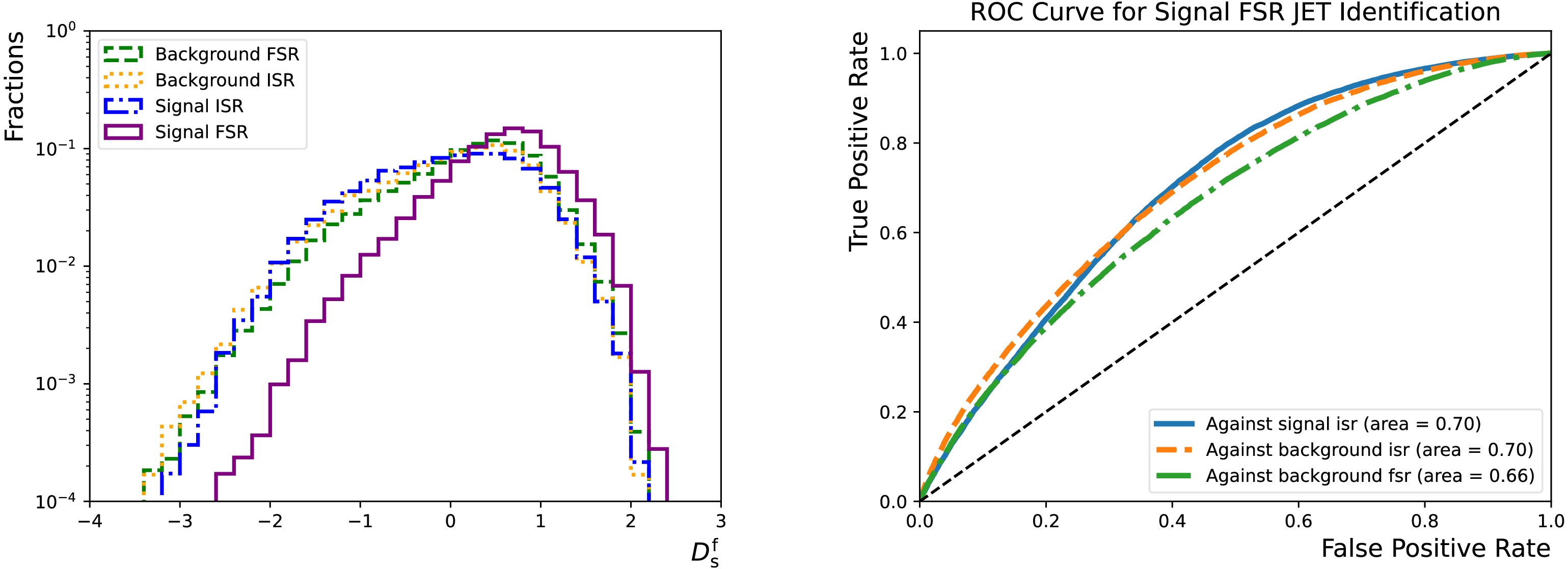
Figure 8. (color online) Left: distributions of
$ D_{{\rm{s}}}^{{\rm{f}}} $ for the "sig-isr" (dotted-dashed line), "sig-fsr" (solid line), "bkg-isr" (dotted line), and "bkg-fsr" (dashed line) categories. Right: "sig-fsr" identification efficiency as functions of the corresponding false positive rates for the "sig-isr" (solid line), "bkg-isr" (dashed line), and "bkg-fsr" (dotted-dashed line) categories. They were evaluated using the test dataset, which accounts for 20% of the total combined dataset. -
The neural network has four output nodes, corresponding to the probabilities for the third jet to be in those four categories: "sig-isr", "sig-fsr", "bkg-isr" and "bkg-fsr". Therefore, they are denoted as
$ p_{{\rm{s}}}^{{\rm{i}}} $ ,$ p_{{\rm{s}}}^{{\rm{f}}} $ ,$ p_{{\rm{b}}}^{{\rm{i}}} $ and$ p_{{\rm{b}}}^{{\rm{f}}} $ , respectively. A discriminating variable can be constructed to balance the target efficiency and the false positive rates:$ D_{{\rm{s}}}^{{\rm{f}}} = \log \dfrac{p_{{\rm{s}}}^{{\rm{f}}}}{(f_{{\rm{s}}}^{{\rm{i}}} \cdot p_{{\rm{s}}}^{{\rm{i}}} + f_{{\rm{b}}}^{{\rm{f}}} \cdot p_{{\rm{b}}}^{{\rm{f}}} + (1 - f_{{\rm{s}}}^{{\rm{i}}} - f_{{\rm{b}}}^{{\rm{f}}}) \cdot p_{{\rm{b}}}^{{\rm{i}}})} $
(1) where
$ f_{{\rm{s}}}^{{\rm{i}}} $ and$ f_{{\rm{b}}}^{{\rm{f}}} $ are hyperparameters that determine the relative importance. This construction is inspired by the flavour tagging algorithms deployed by the ATLAS experiment [44]. It is found that setting$ f_{{\rm{s}}}^{{\rm{i}}} $ ($ f_{{\rm{b}}}^{{\rm{f}}} $ ) to 0.15 (0.7) achieves similar fake rates across different processes for a given efficiency of identifying FSR jets in signal, as seen in Figure 8.
Figure 8. (color online) Left: distributions of the
$ D_{{\rm{s}}}^{{\rm{f}}} $ for the "sig-isr" (dotted-dashed line), "sig-fsr" (solid line), "bkg-isr" (dotted line) and "bkg-fsr" (dashed line) categories. Right: "sig-fsr" identification efficiency as functions of the corresponding false positive rates for the "sig-isr" (solid line), "bkg-isr" (dashed line) and "bkg-fsr" (dotted-dashed line) categories. They are evaluated using the test dataset that accounts for 20% of the total combined dataset. -
The neural network has four output nodes, corresponding to the probabilities for the third jet to be in the four categories "sig-isr," "sig-fsr," "bkg-isr," and "bkg-fsr." Therefore, they are denoted as
$ p_{{\rm{s}}}^{{\rm{i}}} $ ,$ p_{{\rm{s}}}^{{\rm{f}}} $ ,$ p_{{\rm{b}}}^{{\rm{i}}} $ , and$ p_{{\rm{b}}}^{{\rm{f}}} $ , respectively. A discriminating variable can be constructed to balance the target efficiency and false positive rates:$ D_{{\rm{s}}}^{{\rm{f}}} = \log \dfrac{p_{{\rm{s}}}^{{\rm{f}}}}{(f_{{\rm{s}}}^{{\rm{i}}} \cdot p_{{\rm{s}}}^{{\rm{i}}} + f_{{\rm{b}}}^{{\rm{f}}} \cdot p_{{\rm{b}}}^{{\rm{f}}} + (1 - f_{{\rm{s}}}^{{\rm{i}}} - f_{{\rm{b}}}^{{\rm{f}}}) \cdot p_{{\rm{b}}}^{{\rm{i}}})}, $
(1) where
$ f_{{\rm{s}}}^{{\rm{i}}} $ and$ f_{{\rm{b}}}^{{\rm{f}}} $ are hyperparameters that determine the relative importance. This construction is inspired by the flavour tagging algorithms deployed by the ATLAS experiment [44]. It is found that setting$ f_{{\rm{s}}}^{{\rm{i}}} $ ($ f_{{\rm{b}}}^{{\rm{f}}} $ ) to 0.15 (0.7) achieves similar fake rates across different processes for a given efficiency of identifying FSR jets in the signal, as shown in Fig. 8.
Figure 8. (color online) Left: distributions of
$ D_{{\rm{s}}}^{{\rm{f}}} $ for the "sig-isr" (dotted-dashed line), "sig-fsr" (solid line), "bkg-isr" (dotted line), and "bkg-fsr" (dashed line) categories. Right: "sig-fsr" identification efficiency as functions of the corresponding false positive rates for the "sig-isr" (solid line), "bkg-isr" (dashed line), and "bkg-fsr" (dotted-dashed line) categories. They were evaluated using the test dataset, which accounts for 20% of the total combined dataset. -
The application of the classifier can be versatile, but in this study, we use it to correct the reconstructed mass. In an event, if the third jet is identified as coming from the "sig-fsr" category,
$ m_{jj}$ is replaced with the tri-jet invariant mass. The impact of the classifier is three-fold. We expect to obtain improved sensitivity, better$ m_{jj}$ resolutions, and good generality. A high-level discriminant,$ D_{{\rm{s}}}^{{\rm{f}}} $ , is constructed in Formula 1 and can be used to select events for mass correction. The choice of the$ D_{{\rm{s}}}^{{\rm{f}}} $ threshold will affect all three metrics. In fact, in the optimal scenario,$ f_{{\rm{s}}}^{{\rm{i}}} $ and$ f_{{\rm{b}}}^{{\rm{f}}} $ should be tuned for each specific use-case. We perform the optimization sequentially so that$ f_{{\rm{s}}}^{{\rm{i}}} $ ($ f_{{\rm{b}}}^{{\rm{f}}} $ ) is not retuned, and the cut value of$ D_{{\rm{s}}}^{{\rm{f}}} $ is optimized to obtain the best sensitivity. This workflow already gives us significant positive impact. -
The application of the classifier can be versatile, but in this study we use it to correct the reconstructed mass. In an event, if the third jet is identified as coming from the "sig-fsr" category, the
$ m_{{\rm{jj}}}$ is replaced with the tri-jet invariant mass. The impact of the classifier is three-fold. We expect to obtain improved sensitivity, better$ m_{{\rm{jj}}}$ resolutions, and good generality. A high-level discriminant,$ D_{{\rm{s}}}^{{\rm{f}}} $ , is constructed in Formula 1, and can be used to select events for mass correction. The choice of the$ D_{{\rm{s}}}^{{\rm{f}}} $ threshold will affect all three metrics. In fact, in the optimal scenario,$ f_{{\rm{s}}}^{{\rm{i}}} $ and$ f_{{\rm{b}}}^{{\rm{f}}} $ should be tuned for each specific use-case. We perform the optimisation sequentially so that$ f_{{\rm{s}}}^{{\rm{i}}} $ ($ f_{{\rm{b}}}^{{\rm{f}}} $ ) is not retuned, and the cut value of$ D_{{\rm{s}}}^{{\rm{f}}} $ is optimised to obtain the best sensitivity. This workflow already gives us significant positive impact. -
The application of the classifier can be versatile, but in this study, we use it to correct the reconstructed mass. In an event, if the third jet is identified as coming from the "sig-fsr" category,
$ m_{jj}$ is replaced with the tri-jet invariant mass. The impact of the classifier is three-fold. We expect to obtain improved sensitivity, better$ m_{jj}$ resolutions, and good generality. A high-level discriminant,$ D_{{\rm{s}}}^{{\rm{f}}} $ , is constructed in Formula 1 and can be used to select events for mass correction. The choice of the$ D_{{\rm{s}}}^{{\rm{f}}} $ threshold will affect all three metrics. In fact, in the optimal scenario,$ f_{{\rm{s}}}^{{\rm{i}}} $ and$ f_{{\rm{b}}}^{{\rm{f}}} $ should be tuned for each specific use-case. We perform the optimization sequentially so that$ f_{{\rm{s}}}^{{\rm{i}}} $ ($ f_{{\rm{b}}}^{{\rm{f}}} $ ) is not retuned, and the cut value of$ D_{{\rm{s}}}^{{\rm{f}}} $ is optimized to obtain the best sensitivity. This workflow already gives us significant positive impact. -
The sensitivity of the di-jet search can be checked by calculating the significance, defined as
$ \dfrac{{N}_{{\rm{s}}}}{\sqrt{{N}_{{\rm{b}}}}} $ , where$ {N}_{{\rm{s}}} $ ($ {N}_{{\rm{b}}} $ ) is the number of signal (background) events. We consider the binned$ m_{jj}$ , with a universal bin width of 100 GeV, to get the binned significance,$\dfrac{{N}^{\rm i}_{{\rm{s}}}}{\sqrt{{N^{\rm i}}_{{\rm{b}}}}}$ . The highest value,$\max(\dfrac{{N^{\rm i}}_{{\rm{s}}}}{\sqrt{{N^{\rm i}}_{{\rm{b}}}}})$ , is a good indicator of the expected sensitivity. Thus, the optimization of the$ D_{{\rm{s}}}^{{\rm{f}}} $ threshold is performed by a coarse scan to maximize$\max(\dfrac{N^{\rm i}_{\rm s}}{\sqrt{N^{\rm i}_{\rm b}}})$ , considering the nominal test samples. It is found that$ D_{{\rm{s}}}^{{\rm{f}}} = -0.11 $ gives the largest performance gain, where$\max(\dfrac{N^{\rm i}_{\rm s}}{\sqrt{N^{\rm i}_{\rm b}}})$ is improved by 10%−14% for the mass range between 1.5 and 3 TeV, as summarized in Fig. 9. In the analysis, the signal strength is usually extracted via a signal + background fit, where the signal shape also plays a pivotal role. Thus, the actual sensitivity gain will depend on the fit model adopted.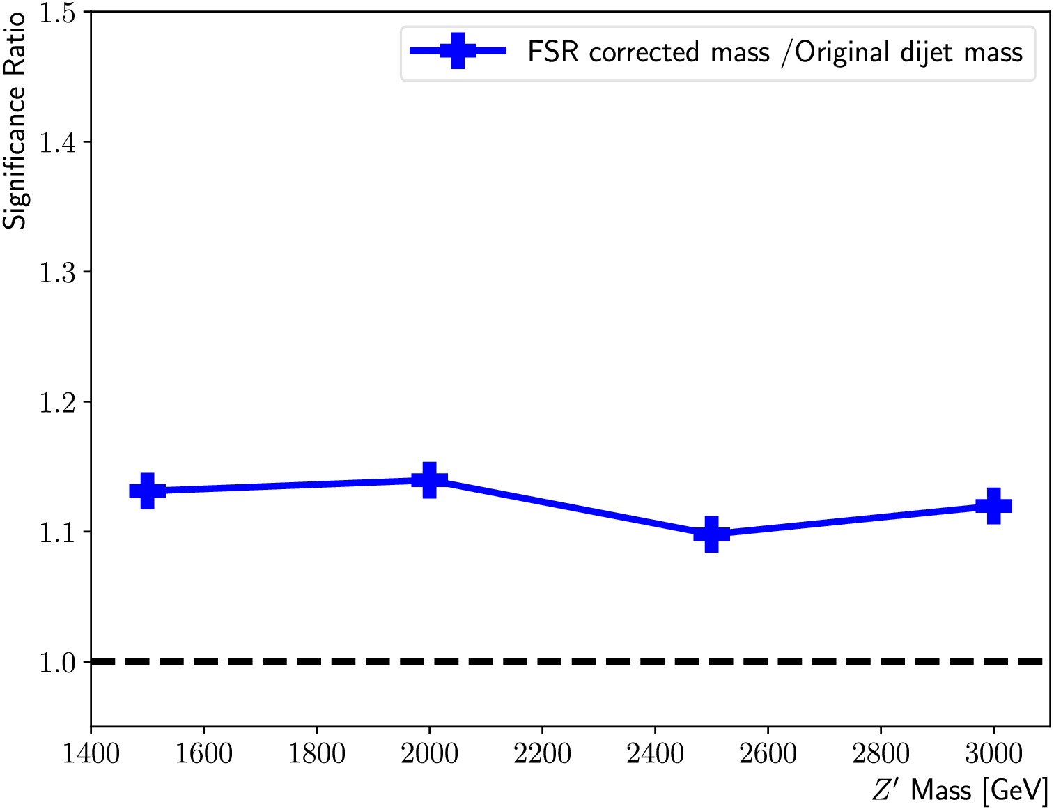
Figure 9. (color online) Summary of the ratios between
$\max(\dfrac{N^{\rm i}_{\rm s}}{\sqrt{N^{\rm i}_{\rm B}}})$ obtained using the FSR corrected mass and that using the original di-jet mass for the$m_{Y_0} $ = 1500, 2000, 2500, and 3000 GeV signal points. -
The sensitivity of the di-jet search can be checked by calculating the significance, defined as
$ \dfrac{{\rm{N}}_{{\rm{s}}}}{\sqrt{{\rm{N}}_{{\rm{b}}}}} $ , where$ {\rm{N}}_{{\rm{s}}} $ ($ {\rm{N}}_{{\rm{b}}} $ ) is the number of signal (background) events. We consider the binned$ m_{{\rm{jj}}}$ , with a universal bin width of 100 GeV, to get the binned significance,$ \dfrac{{\rm{N^i}}_{{\rm{s}}}}{\sqrt{{\rm{N^i}}_{{\rm{b}}}}} $ . The highest value,$ \max(\dfrac{{\rm{N^i}}_{{\rm{s}}}}{\sqrt{{\rm{N^i}}_{{\rm{b}}}}}) $ is a good indicator of the expected sensitivity. So the optimisation of the$ D_{{\rm{s}}}^{{\rm{f}}} $ threshold is done by a coarse scan to maximise$ \max(\dfrac{{\rm{N^i_{s}}}}{\sqrt{{\rm{N^i_{b}}}}}) $ , considering the nominal test samples. It is found that$ D_{{\rm{s}}}^{{\rm{f}}} = -0.11 $ gives the largest performance gain, where$ \max(\dfrac{{\rm{N^i{s}}}}{\sqrt{{\rm{N^i_{b}}}}}) $ is improved by 10-14% for the mass range between 1.5 and 3 TeV, as summarised in Figure 9. In the analysis, the signal strength is usually extracted via a signal + background fit, where the signal shape also plays a pivotal role. So the actual sensitivity gain will depend on the fit model adopted.
Figure 9. (color online) Summary of the ratios between
$ \max(\dfrac{{\rm{N^i_{s}}}}{\sqrt{{\rm{N^i_B}}}}) $ obtained using the FSR corrected mass and that using the original di-jet mass, for the$m_{Y_0} $ = 1500 GeV, 2000 GeV, 2500 GeV and 3000 GeV signal points. -
The sensitivity of the di-jet search can be checked by calculating the significance, defined as
$ \dfrac{{N}_{{\rm{s}}}}{\sqrt{{N}_{{\rm{b}}}}} $ , where$ {N}_{{\rm{s}}} $ ($ {N}_{{\rm{b}}} $ ) is the number of signal (background) events. We consider the binned$ m_{jj}$ , with a universal bin width of 100 GeV, to get the binned significance,$\dfrac{{N}^{\rm i}_{{\rm{s}}}}{\sqrt{{N^{\rm i}}_{{\rm{b}}}}}$ . The highest value,$\max(\dfrac{{N^{\rm i}}_{{\rm{s}}}}{\sqrt{{N^{\rm i}}_{{\rm{b}}}}})$ , is a good indicator of the expected sensitivity. Thus, the optimization of the$ D_{{\rm{s}}}^{{\rm{f}}} $ threshold is performed by a coarse scan to maximize$\max(\dfrac{N^{\rm i}_{\rm s}}{\sqrt{N^{\rm i}_{\rm b}}})$ , considering the nominal test samples. It is found that$ D_{{\rm{s}}}^{{\rm{f}}} = -0.11 $ gives the largest performance gain, where$\max(\dfrac{N^{\rm i}_{\rm s}}{\sqrt{N^{\rm i}_{\rm b}}})$ is improved by 10%−14% for the mass range between 1.5 and 3 TeV, as summarized in Fig. 9. In the analysis, the signal strength is usually extracted via a signal + background fit, where the signal shape also plays a pivotal role. Thus, the actual sensitivity gain will depend on the fit model adopted.
Figure 9. (color online) Summary of the ratios between
$\max(\dfrac{N^{\rm i}_{\rm s}}{\sqrt{N^{\rm i}_{\rm B}}})$ obtained using the FSR corrected mass and that using the original di-jet mass for the$m_{Y_0} $ = 1500, 2000, 2500, and 3000 GeV signal points. -
The sensitivity of the di-jet search can be checked by calculating the significance, defined as
$ \dfrac{{N}_{{\rm{s}}}}{\sqrt{{N}_{{\rm{b}}}}} $ , where$ {N}_{{\rm{s}}} $ ($ {N}_{{\rm{b}}} $ ) is the number of signal (background) events. We consider the binned$ m_{jj}$ , with a universal bin width of 100 GeV, to get the binned significance,$\dfrac{{N}^{\rm i}_{{\rm{s}}}}{\sqrt{{N^{\rm i}}_{{\rm{b}}}}}$ . The highest value,$\max(\dfrac{{N^{\rm i}}_{{\rm{s}}}}{\sqrt{{N^{\rm i}}_{{\rm{b}}}}})$ , is a good indicator of the expected sensitivity. Thus, the optimization of the$ D_{{\rm{s}}}^{{\rm{f}}} $ threshold is performed by a coarse scan to maximize$\max(\dfrac{N^{\rm i}_{\rm s}}{\sqrt{N^{\rm i}_{\rm b}}})$ , considering the nominal test samples. It is found that$ D_{{\rm{s}}}^{{\rm{f}}} = -0.11 $ gives the largest performance gain, where$\max(\dfrac{N^{\rm i}_{\rm s}}{\sqrt{N^{\rm i}_{\rm b}}})$ is improved by 10%−14% for the mass range between 1.5 and 3 TeV, as summarized in Fig. 9. In the analysis, the signal strength is usually extracted via a signal + background fit, where the signal shape also plays a pivotal role. Thus, the actual sensitivity gain will depend on the fit model adopted.
Figure 9. (color online) Summary of the ratios between
$\max(\dfrac{N^{\rm i}_{\rm s}}{\sqrt{N^{\rm i}_{\rm B}}})$ obtained using the FSR corrected mass and that using the original di-jet mass for the$m_{Y_0} $ = 1500, 2000, 2500, and 3000 GeV signal points. -
Applying the above
$ D_{{\rm{s}}}^{{\rm{f}}} $ threshold, the reconstructed mass shows an obviously narrower peak near the actual$m_{Y_0} $ , as shown in Fig. 10. The mild tail above$m_{Y_0} $ comes from ISR jets mis-identified as FSR jets. Figure 11 compares the impact on reconstructed mass, showing that the median is shifted toward$m_{Y_0} $ and the spread becomes smaller.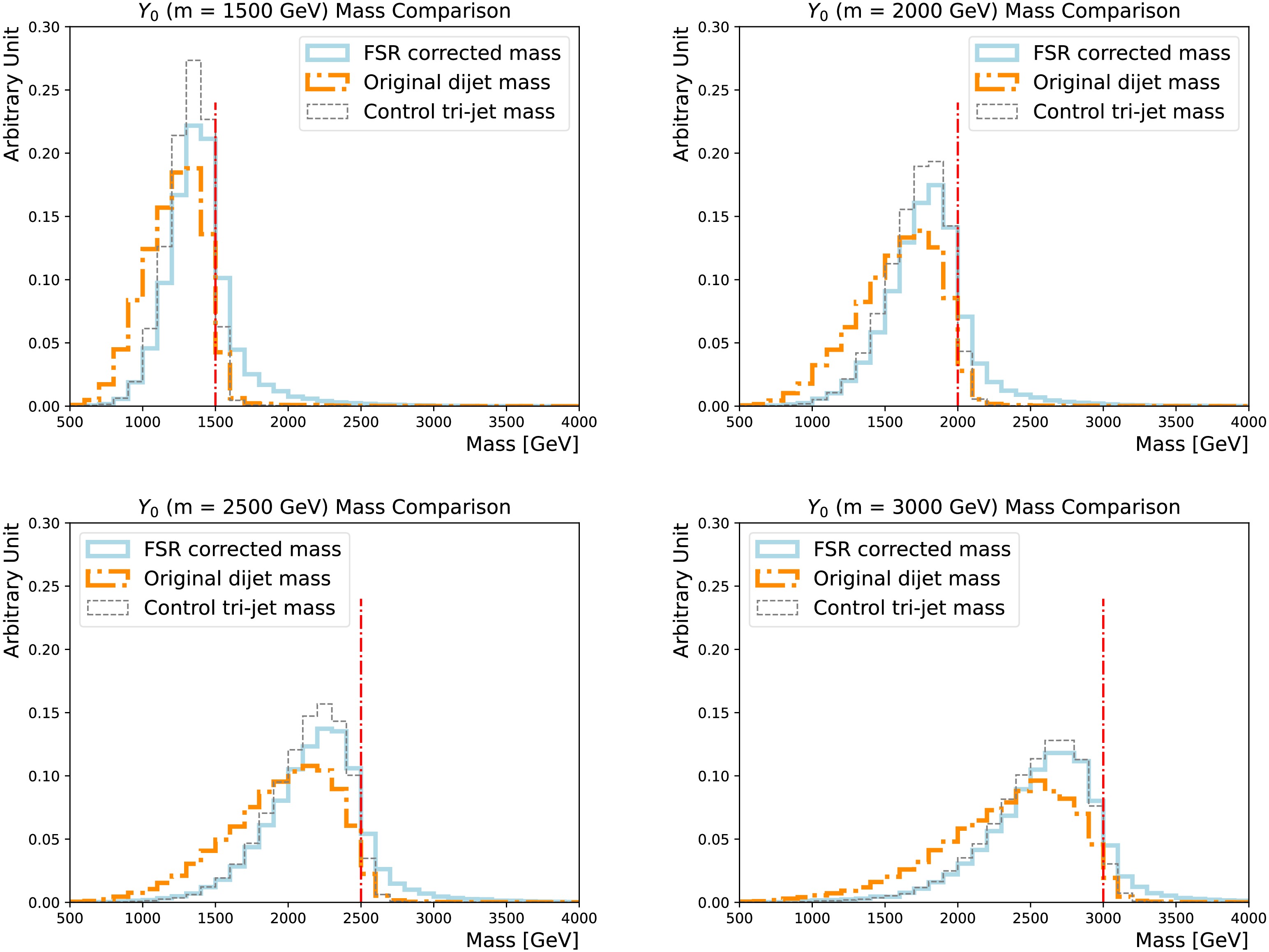
Figure 10. (color online) Comparisons of the FSR corrected masses (solid line) and original di-jet masses (dotted-dashed line) for the
$m_{Y_0} $ = 1500 GeV (upper left), 2000 GeV (upper right), 2500 GeV (lower left), and 3000 GeV (lower right) nominal signal samples. The tri-jet mass calculated using the showering control samples with the FSR/ISR showering switch turned on/off is added as a reference (dashed line). The actual$m_{Y_0} $ is indicated by the vertical line.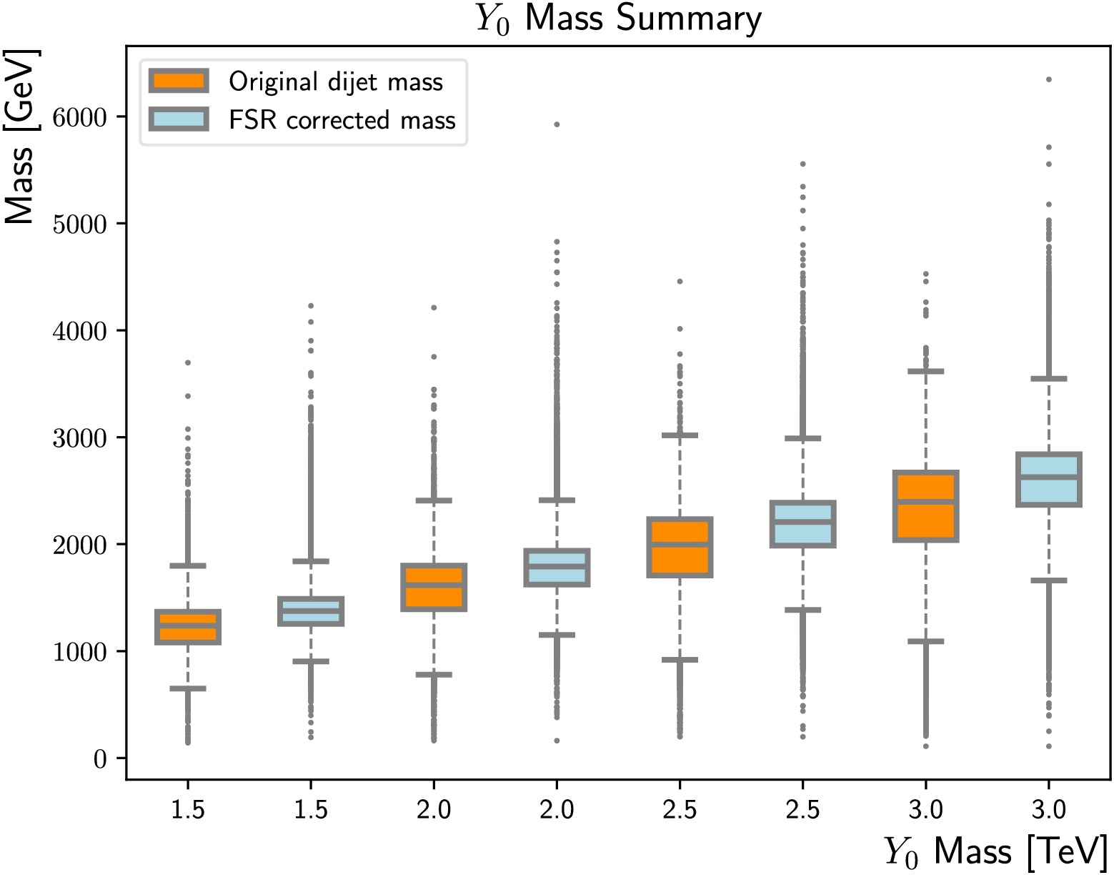
Figure 11. (color online) Summary of the FSR corrected mass distributions (light blue) and original di-jet masses (dark orange) for
$m_{Y_0} $ = 1500, 2000, 2500, and 3000 GeV. The upper/lower boundaries of the boxes indicate the 75%/25% percentile, while the center lines represent the medians. The upper/lower error bars correspond to the 95%/5% percentiles.Because the background estimation methods applied in di-jet resonance searches require the background mass to be smoothly falling, it is pivotal to ensure the algorithm does not have significant mass sculpting. Figure 12 overlays the original
$ m_{jj}$ on the corrected mass for the background process, and both have a smoothly falling behaviour.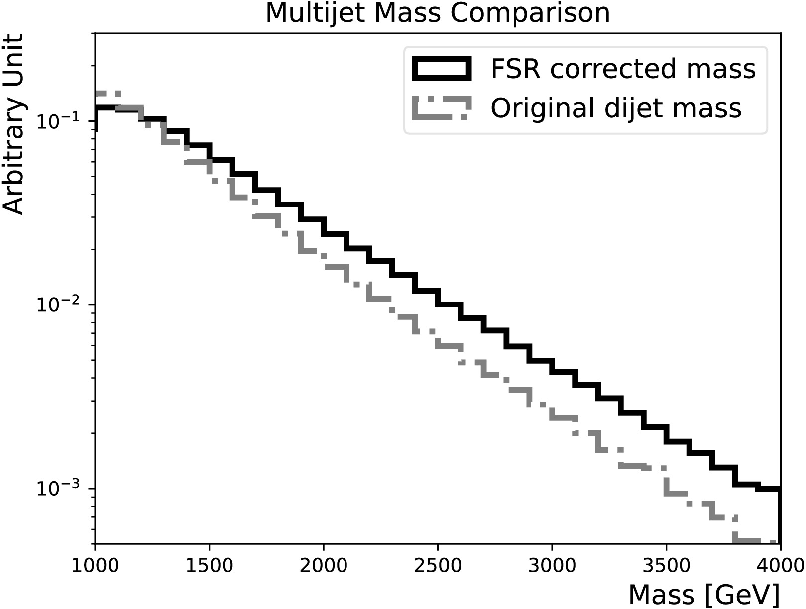
Figure 12. Comparison of the FSR corrected masses (solid line) and original di-jet masses (dotted-dashed line) for the multi-jet background.
The developed method has great flexibilities that allow us to re-optimize the model performance for various scenarios. Two examples are given in Appendix A.
-
Applying the above
$ D_{{\rm{s}}}^{{\rm{f}}} $ threshold, the reconstructed mass shows obviously a narrower peak near the actual$m_{Y_0} $ , as displayed in Figure 10. The mild tail above$m_{Y_0} $ comes from ISR jets mis-identified as FSR jets. Figure 11 compares the impact on reconstructed mass, showing the median is shifted towards$m_{Y_0} $ and the spread becomes smaller.
Figure 10. (color online) Comparisons of the FSR corrected masses (solid line) and the original di-jet masses (dotted-dashed line), for the
$m_{Y_0} $ = 1500 GeV (upper left), 2000 GeV (upper right), 2500 GeV (lower left) and 3000 GeV (lower right) nominal signal samples. The tri-jet mass calculated using the showering control samples with the FSR/ISR showering switch turned on/off is added as a reference (dashed line). The actual$m_{Y_0} $ is indicated by the vertical line.
Figure 11. (color online) Summary of the FSR corrected mass distributions (light blue) and the original di-jet masses (dark orange), for
$m_{Y_0} $ = 1500 GeV, 2000 GeV, 2500 GeV and 3000 GeV. The upper/lower boundary of the box indicates the 75%/25% percentile, while the centre line represents the median. The upper/lower error bar corresponds to the 95%/5% percentile.Since the background estimation methods applied in di-jet resonance searches require the background mass to be smoothly falling, it is pivotal to ensure the algorithm does not have significant mass sculpting. Figure 12 overlays the original
$ m_{{\rm{jj}}}$ and the corrected mass for the background process, and both have a smoothly falling behaviour.
Figure 12. Comparison of the FSR corrected masses (solid line) and the original di-jet masses (dotted-dashed line), for the multi-jet background.
The method developed has great flexibilities that allow us to re-optimise the model performance for various scenarios. Two examples are given in Appendix A.
-
Applying the above
$ D_{{\rm{s}}}^{{\rm{f}}} $ threshold, the reconstructed mass shows an obviously narrower peak near the actual$m_{Y_0} $ , as shown in Fig. 10. The mild tail above$m_{Y_0} $ comes from ISR jets mis-identified as FSR jets. Figure 11 compares the impact on reconstructed mass, showing that the median is shifted toward$m_{Y_0} $ and the spread becomes smaller.
Figure 10. (color online) Comparisons of the FSR corrected masses (solid line) and original di-jet masses (dotted-dashed line) for the
$m_{Y_0} $ = 1500 GeV (upper left), 2000 GeV (upper right), 2500 GeV (lower left), and 3000 GeV (lower right) nominal signal samples. The tri-jet mass calculated using the showering control samples with the FSR/ISR showering switch turned on/off is added as a reference (dashed line). The actual$m_{Y_0} $ is indicated by the vertical line.
Figure 11. (color online) Summary of the FSR corrected mass distributions (light blue) and original di-jet masses (dark orange) for
$m_{Y_0} $ = 1500, 2000, 2500, and 3000 GeV. The upper/lower boundaries of the boxes indicate the 75%/25% percentile, while the center lines represent the medians. The upper/lower error bars correspond to the 95%/5% percentiles.Because the background estimation methods applied in di-jet resonance searches require the background mass to be smoothly falling, it is pivotal to ensure the algorithm does not have significant mass sculpting. Figure 12 overlays the original
$ m_{jj}$ on the corrected mass for the background process, and both have a smoothly falling behaviour.
Figure 12. Comparison of the FSR corrected masses (solid line) and original di-jet masses (dotted-dashed line) for the multi-jet background.
The developed method has great flexibilities that allow us to re-optimize the model performance for various scenarios. Two examples are given in Appendix A.
-
Applying the above
$ D_{{\rm{s}}}^{{\rm{f}}} $ threshold, the reconstructed mass shows an obviously narrower peak near the actual$m_{Y_0} $ , as shown in Fig. 10. The mild tail above$m_{Y_0} $ comes from ISR jets mis-identified as FSR jets. Figure 11 compares the impact on reconstructed mass, showing that the median is shifted toward$m_{Y_0} $ and the spread becomes smaller.
Figure 10. (color online) Comparisons of the FSR corrected masses (solid line) and original di-jet masses (dotted-dashed line) for the
$m_{Y_0} $ = 1500 GeV (upper left), 2000 GeV (upper right), 2500 GeV (lower left), and 3000 GeV (lower right) nominal signal samples. The tri-jet mass calculated using the showering control samples with the FSR/ISR showering switch turned on/off is added as a reference (dashed line). The actual$m_{Y_0} $ is indicated by the vertical line.
Figure 11. (color online) Summary of the FSR corrected mass distributions (light blue) and original di-jet masses (dark orange) for
$m_{Y_0} $ = 1500, 2000, 2500, and 3000 GeV. The upper/lower boundaries of the boxes indicate the 75%/25% percentile, while the center lines represent the medians. The upper/lower error bars correspond to the 95%/5% percentiles.Because the background estimation methods applied in di-jet resonance searches require the background mass to be smoothly falling, it is pivotal to ensure the algorithm does not have significant mass sculpting. Figure 12 overlays the original
$ m_{jj}$ on the corrected mass for the background process, and both have a smoothly falling behaviour.
Figure 12. Comparison of the FSR corrected masses (solid line) and original di-jet masses (dotted-dashed line) for the multi-jet background.
The developed method has great flexibilities that allow us to re-optimize the model performance for various scenarios. Two examples are given in Appendix A.
-
We acknowledge that the above sensitivity assessment metric is rather simple, as in reality, one must perform the actual background estimation. It is expected that in a functional fit, the width of the signal plays a critical role alongside the signal-to-background ratio. In the future, if advanced background modeling methods do not need to assume the background is smoothly falling any more, this methodology has the flexibility to be re-optimized for such a scenario.
The hypothetical
$Y_0 $ particle in the benchmark BSM model has democratic couplings to quarks, and it is not coupled to gluons. Therefore, the only production channel is via$ q\overline{q} $ fusion, and the final state is$ q\overline{q} $ as well. In other theory frameworks, such as the excited quarks [45, 46], extra dimensions [47], and quantum black holes [48], the new particles can couple to both quarks and gluons. Therefore, the production (decay) channels also include gg, gq, and$ g\overline{q} $ . Because the algorithm is trained by utilizing jet mass, a variable correlated with the jet origin, implicitly, its performance is sensitive to the relative fraction between quark-initiated and gluon-initiated jets in the events. The algorithm trained with$Y_0 $ is likely not optimal for those alternative cases. Once including lower level inputs such as the tracks within the jets, the algorithm will have stronger BSM model dependence, which must be carefully considered. Another factor omitted in this study is the interference, either between the ISR and ISR processes or between the signal and multi-jet processes. Such effects have been studied in the past, but they have not been considered in the experiments yet [49−51]. They can potentially become more significant at HL-LHC, so we should pay more attention to them in future investigations.The jet clustering method used is anti-
$ k_t $ [30, 31] with a radius of$ R = 0.4 $ , which is the current standard choice for small-radius jets in both the CMS and ATLAS experiments. It is found that in certain BSM models, such as dark QCD, using a larger jet radius can better reconstruct the heavy particle mass [52, 53]. Furthermore, a large jet radius may mitigate the energy loss due to the FSR, as more final state particles from the heavy particle decay will be clustered. Thus, if a different jet clustering radius is applied, the algorithm must be re-trained, and the conclusion is very likely to change. -
We acknowledge that the above sensitivity assessment metric is rather simple, as in reality one needs to perform the actual background estimation. It is expected that in a functional fit, the width of the signal plays a critical role as well as the signal-to-background ratio. In the future, if advanced background modelling methods do not need to assume the background is smoothly falling any more, this methodology has the flexibility to be re-optimised for such a scenario.
The hypothetical
$Y_0 $ particle in the benchmark BSM model has democratic couplings to quarks, and it is not coupled to gluons. Therefore, the only production channel is via$ q\overline{q} $ fusion, and the final state is$ q\overline{q} $ as well. In other theory frameworks, such as the excited quarks [45, 46], extra dimensions [47] and quantum black holes [48], the new particles can couple to both quarks and gluons. So the production (decay) channels also include gg, gq and$ g\overline{q} $ . Since the algorithm is trained utilising jet mass, a variable correlated with the jet origin, implicitly, its performance is sensitive to the relative fraction between quark-initiated and gluon-initiated jets in the events. The algorithm trained with$Y_0 $ is likely not optimal for those alternative cases. Once including lower level inputs such as the tracks within the jets, the algorithm will have stronger BSM model dependence, which has to be carefully thought of. Another factor omitted in this study is the interference, either between the ISR and ISR processes, or between the signal and multi-jet processes. Such effects have been studied in the past, but they have not been considered in the experiments yet [49−51]. They can potentially become more significant at HL-LHC, so we should pay more attention in future investigations.The jet clustering method used is anti-
$ k_t $ [30, 31] with a radius of$ R = 0.4 $ , which is the current standard choice for small-radius jets in both the CMS and ATLAS experiments. It is found that in certain BSM models such as dark QCD, using a larger jet radius can better reconstruct the heavy particle mass [52, 53]. Furthermore, a large jet radius may mitigate the energy loss due to the FSR, as more final state particles from the heavy particle decay will be clustered. So if a different jet clustering radius is applied, the algorithm has to be re-trained, and very likely the conclusion will change. -
A classifier is developed to identify FSR jets in
$Y_0 $ events while rejecting both the ISR jets in$Y_0 $ and FSR/ISR jets in a multi-jet background. The identified signal FSR jet is used to correct the reconstructed mass, which improves the mass resolution and sensitivity. It uses only the variables that are not sensitive to$ m_{jj}$ , so an improvement of 12%−20% in sensitivity is observed across a large mass region.It is remarkable that only using the 4-momenta of the leading three jets already ensures promising performance. The classifier can achieve a 40% signal FSR jet identification efficiency, while the fake rate of the other sources is at the
$ \sim 20 $ % level by constructing the discriminant accordingly. The classifier can be flexibly adapted to different goals, either focusing on the signal mass resolutions or sensitivity. It is possible to utilize more fundamental quantities, such as the charged particles or calorimeter deposits, to explore color connections [22, 34, 35], but the showering and detector dependence must be evaluated.The LHC will conclude Run-3 data-taking in the near future, and eventually, we have to embrace the HL-LHC era. To achieve the ultimate sensitivity at the HL-LHC, we need to maximize the discovery potential. FSR tagging offers a way to further enhance the sensitivities, and it can be embedded in a multi-class categorization task to satisfy various analysis goals. The di-jet resonance search has been the flagship inclusive search among hadron colliders. Despite its long history, there is still space to enhance its potential, particularly with modern ML-based technologies. The idea explored in this work may be extended to other topics in the hadronic final states. We look forward to seeing such techniques tested by the experiments.
-
A classifier is developed to identify FSR jets in
$Y_0 $ events while rejecting both the ISR jets in$Y_0 $ and FSR/ISR jets in multi-jet background. The identified signal FSR jet is used to correct the reconstructed mass, which improves the mass resolution and the sensitivity. It uses only the variables that are not sensitive to$ m_{{\rm{jj}}}$ , so an improvement of 12-20% in sensitivity is observed across a large mass region.It is remarkable that only using the 4-momenta of the leading three jets already ensures promising performance. The classifier can achieve a 40% signal FSR jet identification efficiency while the fake rate of the other sources is at
$ \sim 20 $ % level, by constructing the discriminant accordingly. The classifier is flexible to be adapted for different goals, either focusing on the signal mass resolutions or the sensitivity. It is possible to utilise more fundamental quantities, such as the charged particles or the calorimeter deposits, to explore colour connections [22, 34, 35], but the showering and detector dependence have to be evaluated.The LHC will conclude Run-3 data-taking in the near future, and eventually, we have to embrace the HL-LHC era. To achieve the ultimate sensitivity at the HL-LHC, we need to maximise the discovery potential. FSR tagging offers a way to further enhance the sensitivities, and it can be embedded in a multi-class categorisation task to satisfy various analysis goals. The di-jet resonance search has been the flagship inclusive search in hadron colliders. Despite its long history, there is still space to enhance its potential, in particular with modern ML-based technologies. The idea explored in this work may be extended to other topics in the hadronic final states. We look forward to seeing such techniques tested by the experiments.
-
We thank Sascha Dreyer, Christian Sander, Ryo Ishikawa, and Yohei Yamaguchi for very constructive discussions. We also thank Marco Montella and Antonio Boveia for pointing relevant references to us. As undergraduates, Y.X. Shen and Y.S.Z. Sui contributed to sample generation, kinematic studies, and the algorithm training/ testing for this work substantially.
-
We thank Sascha Dreyer, Christian Sander, Ryo Ishikawa and Yohei Yamaguchi for very constructive discussions. We also thank Marco Montella and Antonio Boveia for pointing relevant references to us. As undergraduates, Y.X. Shen and Y.S.Z. Sui contributed to sample generation, kinematic studies and the algorithm training/testing for this work substantially.
-
We thank Sascha Dreyer, Christian Sander, Ryo Ishikawa, and Yohei Yamaguchi for very constructive discussions. We also thank Marco Montella and Antonio Boveia for pointing relevant references to us. As undergraduates, Y.X. Shen and Y.S.Z. Sui contributed to sample generation, kinematic studies, and the algorithm training/ testing for this work substantially.
-
The generality of the classifier is assessed using signal points, with
$m_{Y_0} $ ranging from 3.5 to 5 TeV, that are not included in the training. Since variables strongly correlated with the mass are excluded from the training, and the training datasets are sampled to evenly populated in jet$p_{{\rm{T}}} $ , the classifier brings similar sensitivity gains and mass resolution improvements in the high mass region as well, seen in Figure figs. 13 to 15.
Figure 13. (color online) Summary of the ratios between
$ \max(\dfrac{{\rm{N^i_{s}}}}{\sqrt{{\rm{N^i_B}}}}) $ obtained using the FSR corrected mass and that using the original di-jet mass, for the$m_{Y_0} $ = 3500 GeV, 4000 GeV, 4500 GeV and 5000 GeV signal points.
Figure 14. (color online) Comparisons of the FSR corrected masses (solid line) and the original di-jet masses (dotted-dashed line), for the
$m_{Y_0} $ = 3500 GeV (upper left), 4000 GeV (upper right), 4500 GeV (lower left) and 5000 GeV (lower right) nominal signal samples. The tri-jet mass calculated using the showering control samples with the FSR/ISR showering switch turned on/off is added as a reference (dashed line). The actual$m_{Y_0} $ is indicated by the vertical line.
Figure 15. (color online) Summary of the FSR corrected mass distributions (light blue) and the original di-jet masses (dark orange), for
$m_{Y_0} $ = 3500 GeV, 4000 GeV, 4500 GeV and 5000 GeV. The upper/lower boundary of the box indicates the 75%/25% percentile, while the centre line represents the median. The upper/lower error bar corresponds to the 95%/5% percentile. -
The generality of the classifier is assessed using signal points, with
$m_{Y_0} $ ranging from 3.5 to 5 TeV, that are not included in the training. Because variables strongly correlated with the mass are excluded from the training and the training datasets are sampled to be evenly populated in jet$p_{T} $ , the classifier brings similar sensitivity gains and mass resolution improvements in the high mass region as well, as shown in Figs. A1 to A3.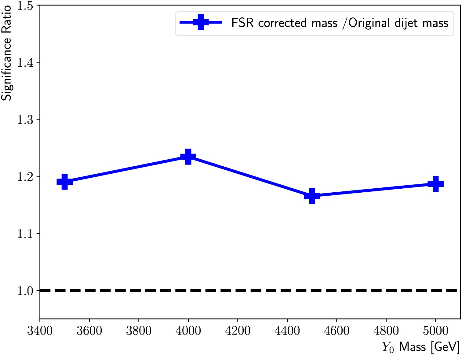
Figure A1. (color online) Summary of the ratios between
$\max(\dfrac{N^{\rm i}_{\rm s}}{\sqrt{N^{\rm i}_{\rm B}}})$ obtained using the FSR corrected mass and using the original di-jet mass for the$m_{Y_0} $ = 3500 GeV, 4000 GeV, 4500 GeV, and 5000 GeV signal points.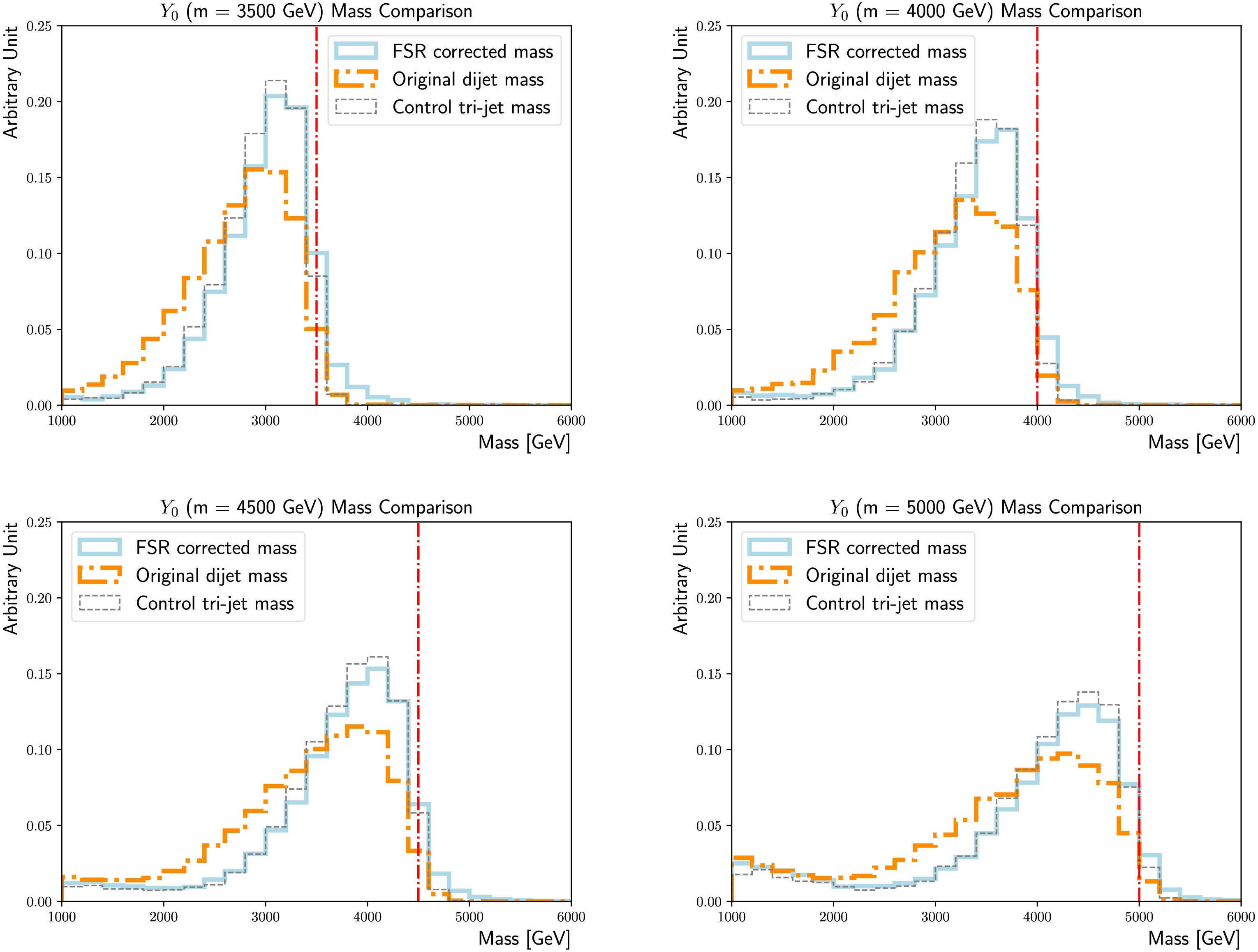
Figure A2. (color online) Comparisons of the FSR corrected masses (solid line) and original di-jet masses (dotted-dashed line) for the
$m_{Y_0} $ = 3500 GeV (upper left), 4000 GeV (upper right), 4500 GeV (lower left), and 5000 GeV (lower right) nominal signal samples. The tri-jet mass calculated using the showering control samples with the FSR/ISR showering switch turned on/off is added as a reference (dashed line). The actual$m_{Y_0} $ is indicated by the vertical line.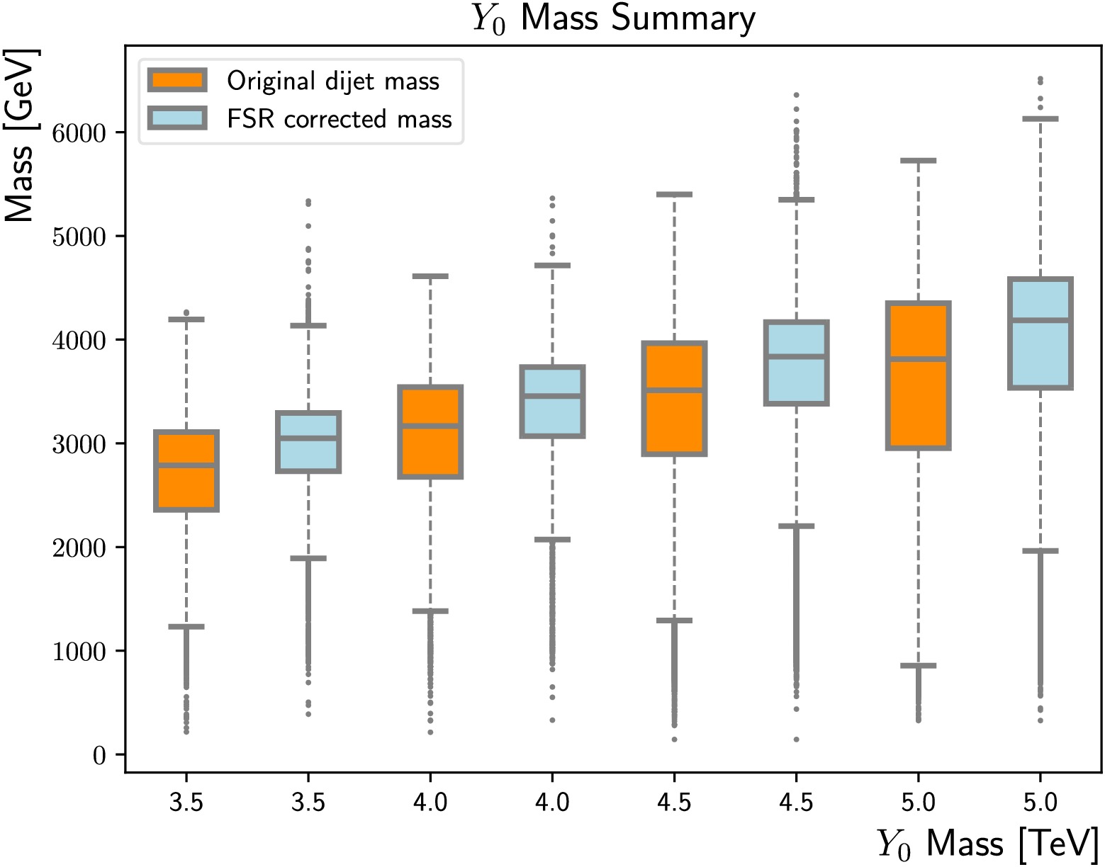
Figure A3. (color online) Summary of the FSR corrected mass distributions (light blue) and original di-jet masses (darkorange), for
$m_{Y_0} $ = 3500 GeV, 4000 GeV, 4500 GeV, and 5000 GeV. The upper/lower boundaries of the boxes indicate the 75%/25% percentiles, while the centre lines represent the median. The upper/lower error bars correspond to the 95%/5% percentiles. -
The relative fractions,
$ f_{{\rm{s}}}^{{\rm{i}}} $ and$ f_{{\rm{b}}}^{{\rm{f}}} $ , in the definition of$ D_{{\rm{s}}}^{{\rm{f}}} $ can be re-tuned for alternative use cases. In Section IV.C, they were chosen so that the classifier achieves similar false positive rates for all three categories, besides "sig-fsr." This choice is motivated by the requirement that the background mass spectrum should not be altered significantly. In a hypothetical case where such constraints are mitigated, either due to advanced background modelling techniques or analysis strategies, the classifier can be made to fully concentrate on distinguishing "sig-fsr" from "sig-isr" by setting$ f_{{\rm{s}}}^{{\rm{i}}} $ ($ f_{{\rm{b}}}^{{\rm{f}}} $ ) to 1 (0). Figure A4 shows the corresponding$ D_{{\rm{s}}}^{{\rm{f}}} $ distributions and ROC curves. Clearly, the rejection against "sig-isr" is significantly enhanced compared to that in Fig. 8.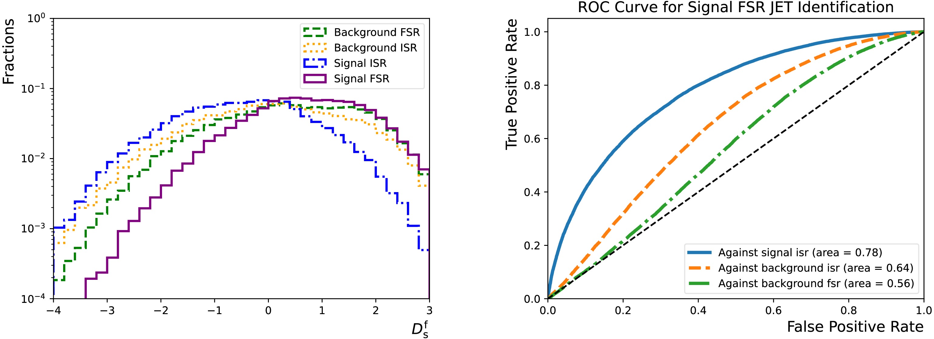
Figure A4. (color online) Left: Distributions of
$ D_{{\rm{s}}}^{{\rm{f}}} $ for the "sig-isr" (dotted-dashed line), "sig-fsr" (solid line), "bkg-isr" (dotted line), and "bkg-fsr" (dashed line) categories. Right: "sig-fsr" identification efficiency as functions of the corresponding false positive rates for the "sig-isr" (solid line), "bkg-isr" (dashed line), and "bkg-fsr" (dotted-dashed line) categories. They are evaluated using the test dataset that accounts for 20% of the total combined dataset.$ f_{{\rm{s}}}^{{\rm{i}}} $ ($ f_{{\rm{b}}}^{{\rm{f}}} $ ) are set to 1 (0). -
The relative fractions,
$ f_{{\rm{s}}}^{{\rm{i}}} $ and$ f_{{\rm{b}}}^{{\rm{f}}} $ , in the definition of$ D_{{\rm{s}}}^{{\rm{f}}} $ , can be re-tuned for alternative use cases. In Section 4.3, they were chosen so that the classifier achieves similar false positive rates for all the three categories, besides "sig-fsr". This choice is motivated by the requirement that the background mass spectrum should not be altered significantly. In a hypothetical case where such constraints are mitigated, either due to advanced background modelling techniques or analysis strategies, the classifier can be made fully concentrated on distinguishing "sig-fsr" from "sig-isr", by setting$ f_{{\rm{s}}}^{{\rm{i}}} $ ($ f_{{\rm{b}}}^{{\rm{f}}} $ ) to 1 (0). Figure 16 shows the corresponding$ D_{{\rm{s}}}^{{\rm{f}}} $ distributions and the ROC curves. Clearly, the rejection against "sig-isr" is significantly enhanced compared to that in Figure 8.
Figure 16. (color online) Left: Distributions of the
$ D_{{\rm{s}}}^{{\rm{f}}} $ for the "sig-isr" (dotted-dashed line), "sig-fsr" (solid line), "bkg-isr" (dotted line) and "bkg-fsr" (dashed line) categories. Right: "sig-fsr" identification efficiency as functions of the corresponding false positive rates for the "sig-isr" (solid line), "bkg-isr" (dashed line) and "bkg-fsr" (dotted-dashed line) categories. They are evaluated using the test dataset that accounts for 20% of the total combined dataset.$ f_{{\rm{s}}}^{{\rm{i}}} $ ($ f_{{\rm{b}}}^{{\rm{f}}} $ ) are set to 1 (0). -
The relative fractions,
$ f_{{\rm{s}}}^{{\rm{i}}} $ and$ f_{{\rm{b}}}^{{\rm{f}}} $ , in the definition of$ D_{{\rm{s}}}^{{\rm{f}}} $ can be re-tuned for alternative use cases. In Section IV.C, they were chosen so that the classifier achieves similar false positive rates for all three categories, besides "sig-fsr." This choice is motivated by the requirement that the background mass spectrum should not be altered significantly. In a hypothetical case where such constraints are mitigated, either due to advanced background modelling techniques or analysis strategies, the classifier can be made to fully concentrate on distinguishing "sig-fsr" from "sig-isr" by setting$ f_{{\rm{s}}}^{{\rm{i}}} $ ($ f_{{\rm{b}}}^{{\rm{f}}} $ ) to 1 (0). Figure A4 shows the corresponding$ D_{{\rm{s}}}^{{\rm{f}}} $ distributions and ROC curves. Clearly, the rejection against "sig-isr" is significantly enhanced compared to that in Fig. 8.
Figure A4. (color online) Left: Distributions of
$ D_{{\rm{s}}}^{{\rm{f}}} $ for the "sig-isr" (dotted-dashed line), "sig-fsr" (solid line), "bkg-isr" (dotted line), and "bkg-fsr" (dashed line) categories. Right: "sig-fsr" identification efficiency as functions of the corresponding false positive rates for the "sig-isr" (solid line), "bkg-isr" (dashed line), and "bkg-fsr" (dotted-dashed line) categories. They are evaluated using the test dataset that accounts for 20% of the total combined dataset.$ f_{{\rm{s}}}^{{\rm{i}}} $ ($ f_{{\rm{b}}}^{{\rm{f}}} $ ) are set to 1 (0). -
The relative fractions,
$ f_{{\rm{s}}}^{{\rm{i}}} $ and$ f_{{\rm{b}}}^{{\rm{f}}} $ , in the definition of$ D_{{\rm{s}}}^{{\rm{f}}} $ can be re-tuned for alternative use cases. In Section IV.C, they were chosen so that the classifier achieves similar false positive rates for all three categories, besides "sig-fsr." This choice is motivated by the requirement that the background mass spectrum should not be altered significantly. In a hypothetical case where such constraints are mitigated, either due to advanced background modelling techniques or analysis strategies, the classifier can be made to fully concentrate on distinguishing "sig-fsr" from "sig-isr" by setting$ f_{{\rm{s}}}^{{\rm{i}}} $ ($ f_{{\rm{b}}}^{{\rm{f}}} $ ) to 1 (0). Figure A4 shows the corresponding$ D_{{\rm{s}}}^{{\rm{f}}} $ distributions and ROC curves. Clearly, the rejection against "sig-isr" is significantly enhanced compared to that in Fig. 8.
Figure A4. (color online) Left: Distributions of
$ D_{{\rm{s}}}^{{\rm{f}}} $ for the "sig-isr" (dotted-dashed line), "sig-fsr" (solid line), "bkg-isr" (dotted line), and "bkg-fsr" (dashed line) categories. Right: "sig-fsr" identification efficiency as functions of the corresponding false positive rates for the "sig-isr" (solid line), "bkg-isr" (dashed line), and "bkg-fsr" (dotted-dashed line) categories. They are evaluated using the test dataset that accounts for 20% of the total combined dataset.$ f_{{\rm{s}}}^{{\rm{i}}} $ ($ f_{{\rm{b}}}^{{\rm{f}}} $ ) are set to 1 (0).
Enhancing di-jet resonance searches via a final-state radiation jet tagging algorithm
- Received Date: 2025-10-18
- Available Online: 2026-04-15
Abstract: In this study, we investigate the possibility of enhancing the di-jet resonance searches by tagging the final state radiation (FSR) jet using an event-level deep neural network. It is found that solely relying on the 4-momenta of the leading three jets allows the algorithm to achieve good discriminating power that can identify the hardest FSR jet in the signal while rejecting other soft jets. Once the invariant mass is corrected with the tagged FSR jet, the mass resolution of the signal is greatly enhanced, and the sensitivity of the search is also improved by more than 10%. By crafting the input variables carefully, the algorithm introduces minimal mass sculpting for the background, and its applicability extends to a broad mass range. This work proves that FSR jet tagging can potentially enhance di-jet resonance searches, suiting various stages of the physics programmes at the Large Hadron Collider (LHC) and High-Luminosity LHC (HL-LHC).


 DownLoad: