Study of color-flavor locked quark stars in ${\boldsymbol f(R,L_{m},T)}$ gravity using observational data

The birth of general relativity (GR) had a profound impact on the theory of gravity, astrophysics, and cosmology. Based on Einstein's field equations and cosmological principles, the standard Big Bang model of the universe was established and later validated by observations such as the cosmic microwave background radiation and Hubble's law. However, in the 1990s, observations of Type Ia supernovae revealed that the universe was expanding at an accelerated rate, which challenged the original model [1, 2]. To explain this phenomenon, the standard model introduced dark energy, a hypothetical mysterious substance with negative pressure. Alternatively, some researchers proposed that the accelerated expansion could be explained by modifying gravitational theories without introducing new components of matter. As a result, many modified gravitational theories were proposed, such as the scalar-tensor theory [3, 4], Hořava-Lifshitz theory [5, 6], Eddington-inspired Born-Infeld theory [7, 8], dRGT massive theory [9, 10], etc., which provide different theoretical paths for the accelerated expansion of the universe.

One of the simplest modified theories of gravity is $ f(R) $ gravity [11−15], which is achieved by replacing the Ricci scalar R in the gravitational action with an arbitrary function $ f(R) $. Building upon this foundation, Harko et al.proposed two extensions: $ f(R, L_{m}) $ gravity [16, 17] and $ f (R, T) $ gravity [18, 19]. More recently, Haghani and Harko proposed a broader theoretical framework known as the $ f(R,L_{m},T) $ theory of gravity [20], which incorporates both the matter Lagrangian density $ L_{m} $ and the trace of energy-momentum tensor T into the gravitational action. These modified gravity theories have been widely applied to the study of compact stars, offering new insights into stellar collapse and stability problems. For example, perturbative modeling of $ f(R) $ gravity has been applied to study neutron stars [21]. Furthermore, higher-order $ f(R) $ gravity can also solve problems associated with supermassive neutron stars [22]. Aman et al. analyzed neutron stars within the framework of $ f(R,G,L_{m}) $ gravity [23]. The neutron stars and wormhole in the $ f(R,L_{m}) $ gravity [24, 25] and $ f(R,T) $ gravity [26, 27] was investigated. In $ f(R,L_{m},T) $ theory of gravity, researchers explored the wormhole [28−31] and neutron stars [32].

In the latest experimental observations, the mass limits of massive pulsars impose stringent constraints on the equation of state of compact stars. For example, PSR J1614-2230, which was observed in 2010 [33], has a mass of approximately 2.0 solar mass, challenging many traditional nuclear equation of state models. The LIGO/Virgo Collaboration measured the secondary object in the gravitational wave event GW190814, which has a mass between 2.5 and 2.67 solar masses [34], lying in the so-called mass gap region between the heaviest known neutron stars and the lightest black holes. The specific nature of these stars remains unclear, further stimulating interest in the study of strange stars. It is believed that the interior of neutron stars may be composed of more tightly bound nucleons, or even absolutely stable strange quark matter. Quark stars, theoretically composed of strange quark matter, could also exist [35−38]. The quark matter in strange quark stars is electrically neutral, composed of β -equilibrium u, d, s quarks as well as electrons and muons [39−41]. The MIT bag model is a simple and effective method to describe strange quark matter, where quarks are assumed to move freely within a spherical region. Based on the equation of state of this model, Maurya et al. modeled compact objects using the gravitational decoupling method [42−44]. Many researchers explored the structure and stability of strange quark stars in the framework of GR [45−48] and modified gravitational theories [49−64].

On the other hand, color-flavor locked (CFL) quark matter is considered to the most symmetric ground state [65, 66], which is likely to exist in hybrid stars or quark stars [67]. If CFL quark matter is considered in compact stars, the number density of the u, d, and s quarks will be equal, and no leptons will be contained in the CFL state. CFL quark matter could be more stable than strange quark matter [68]. Recent studies suggest that CFL quark matter can explain the secondary companion of the GW190814 event and observations such as HESS J1731-347 [69−72]. Bora et al. studied CFL quark stars and their gravitational wave echoes in Rastall gravity [73]. Moreover, the properties of CFL quark stars in the modified gravitational theory were explored in Refs. [74−81] using observations of massive pulsars. In this paper, we study the properties of CFL quark stars within the framework of $ f(R,L_{m},T) $ gravity, based on observational constraints from massive pulsars PSR J0740-6620, PSR J0952-0607, PSR J1614-2230, and the GW190814 event.

This paper focuses on the properties of CFL quark stars within the framework of $ f(R, L_m, T) $ gravity, a theory that formally unifies and extends the $ f(R,T) $ and $ f(R,L_m) $ models. We adopt the specific form $ f(R, L_m, T) = R + \alpha T L_m $ to investigate the effect of the free parameter α on the mass and radius of quark stars. Furthermore, we fit several observed compact stars and present radius predictions under different parameter conditions to assess the explanatory power of this theory with respect to astronomical observations.

The structure of the paper is as follows: we begin with a brief overview of $ f(R,L_{m},T) $ gravity and the modified TOV equation. Sec. III introduces the equation of state for the CFL phase of quark matter. In Sec. IV, we employ numerical methods to investigate the structure of quark stars in $ f(R,L_{m},T) $ gravity, focusing on the impact of free parameters on key properties such as the mass-radius relation, compactness, gravitational redshift and dynamical stability. Finally, conclusions are given in Sec. V.

The action of $ f(R,L_{m},T) $ theory of gravity is written as [20]

By varying the action S with respect to the metric g, we obtain

where we defined $ f_{R}\equiv\partial f/\partial R $, $ f_{L}\equiv\partial f/\partial L_{m} $ and $ f_{T}\equiv\partial f/\partial T $. The variation of the Ricci scalar are derived from the Palatini identity for the Ricci scalar, namely

where $ \nabla_{\alpha} $ is the covariant derivative and $ R_{\mu\nu} $ is the Ricci tensor. The field equations is written as

where $ \tau_{\mu\nu} $ is defined as

Let's begin by applying the covariant derivative of Eq. (4)

Using the geometric identity $ \nabla^{\mu}G_{\mu\nu}=0 $ and the mathematical property $(\Box\nabla_{\nu}-\nabla_{\nu}\Box)f_{R}=R_{\mu\nu}\nabla^{\nu}f_{R} $, we obtain the equation for the covariant derivative of the energy-momentum tensor as:

where we define

To study the structure of quark stars in the above modified gravitational theory, the following form of an arbitrary function is considered

in which α is matter geometry coupling constant. Eq. (4) is written as

Until 1939, there were only two analytical solutions to Einstein's field equations: one was Einstein's cosmological solution, and the other was Schwarzschild's internal solution for an incompressible fluid sphere. Tolman was the first to propose a new analytical solution to Einstein's field equations: the static solution of the fluid sphere. Oppenheimer and Volkoff immediately applied this solution to the to calculations of the structure of neutron stars, which led to the development of the static equilibrium equations for fluids, known as the TOV equations. In the following, we present the modified TOV equations within the framework of $ f(R,L_{m},T) $ gravity.

For a static sphere with a symmetric distribution of matter, we use the following line element:

where ν and λ are radial functions. The energy-momentum tensor can be expressed as

where ρ and p denote the energy density and pressure of the fluid, respectively, and $ u_{\mu} $ is the quadratic velocity. Therefore, we obtain

The matter Lagrangian density typically has two possible forms, namely $ L_{m}=-\rho $ and $ L_{m}=p $. Different forms of the Lagrangian density not only simplify the expression of the field equations but also influence the internal structural properties of compact objects (for more discussion on this topic, see Ref. [82] for more discussion). In this study, we choose the matter Lagrangian density as $ L_{m}=-\rho $ and combine it with Eq. (13), thus simplifying the field equation Eq. (10) to

By using the field equation Eq. (14) and spherical symmetry metric Eq. (11), the nonzero component of the field equation can be calculated with the following expression

Here, the prime represents the derivative with respect to r. Taking the covariant divergence of Eq. (7), we obtain

Similarly to the form of GR, the metric function $ \lambda(r) $ is defined as

Subsequently, combining Eqs. (15)-(17), Eq. (18), and Eq. (19), we ultimately conclude that [32]

To recover the standard TOV equation in GR from Eq. (21), all that is needed is that $ \alpha = 0 $.

In quark matter, the three quark flavors are considered to be equivalent when the density is sufficiently high and the breaking effect of the strange quark mass is negligible. At this point, all three colors and all three flavors are fully paired. The three flavor quarks form conventional zero-momentum, spinless Cooper pairs, quark condensation is not invariant under either color or flavor transformations alone. However, it is invariant under simultaneous color and flavor transformations, meaning that the condensation locks the color and flavor degrees of freedom together, and the Fermi momentum of all the flavors becomes a same value, which corresponds to the CFL phase. CFL phase quark matter reduces the free energy of quark matter by adding an energy gap term to free-state quark matter. The thermodynamic potential of this form can be expressed as by [83]

where Δ is the energy gap, B is the bag pressure. $ \Omega_{free} $ denotes the free energy of non-interacting quarks, which is expressed as follows

where μ represents the baryon chemical potential, which is expressed as $ \mu= (\mu_{u} + \mu_{d} + \mu_{s})/3 $, $ m_{s} $ denotes the mass of the strange quark. All quarks share the same Fermi momentum ν, and all participate in the pairing, so they have the same quark number density n $(=n_{u}=n_{d}=n_{s}) $. ν and n are given by

The pressure and energy density of the CFL quark matter phase can be expressed as

The equation of state can now be expressed as:

where σ is defined by

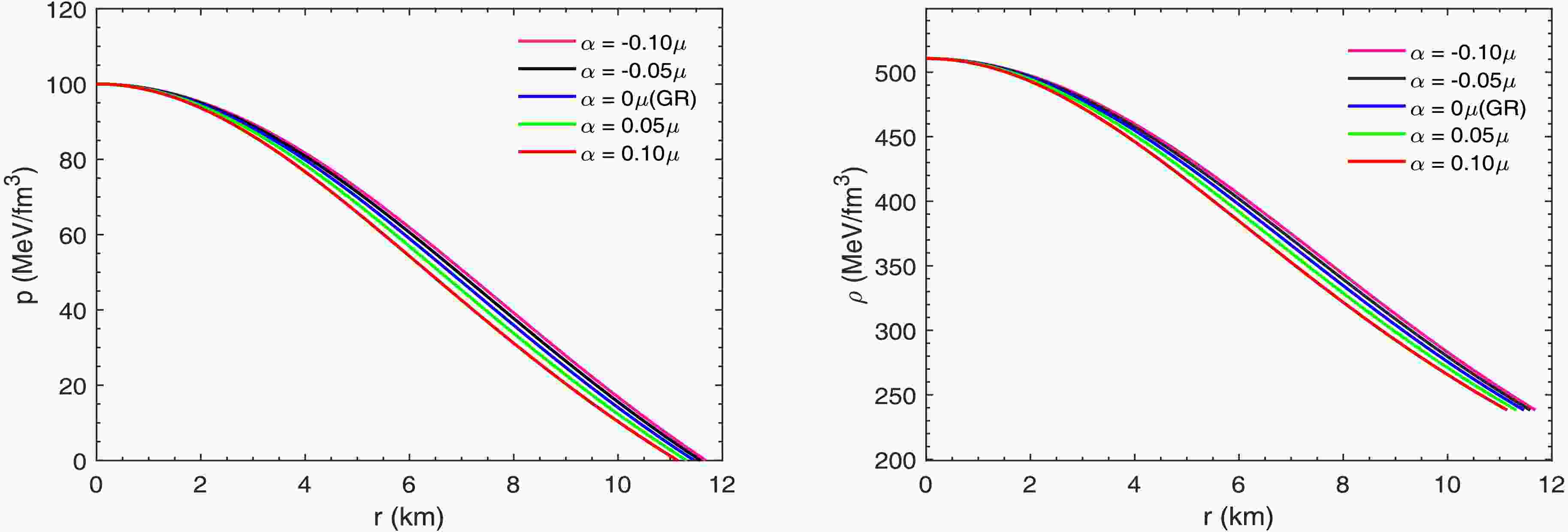
Since TOV equation (21) and the mass function equation (20) are highly nonlinear and difficult to solve analytically, we use numerical integration to solve them. These two equations involve three unknown quantities: $ m(r) $, $ \rho(r) $, and $ p(r) $, Therefore, we need to introduce the formula that describes the relationship between pressure and density inside the star, i.e., the equation of state of CFL quark matter. Given that these are first-order differential equations, two boundary conditions need to be specified, namely $ M(0) = 0 $ and $ \rho(0) = \rho_{c} $, where $ \rho_{c} $ is the central energy density. The integration process ends at the surface of the star ($ p(R) = 0 $), where R is the radius of the quark star, and the corresponding mass $ M(R) $ represents the total mass of the star. To facilitate the solution, we convert the units in the equation of state, the mass function equation, and the TOV equation. In this formulation, the gravitational parameter α has units of μ, where $ \mu = 10^{-78} $ s$ ^{4} $/kg$ ^{2} $.

In order to examine the feasibility of the quark star model, we show the variation of the energy density and pressure inside the quark star for different gravitational parameters α in Fig. 1. The results show that both the pressure and the center density are nonsingular. We also observe that the radius of the star decreases gradually with increasing α.

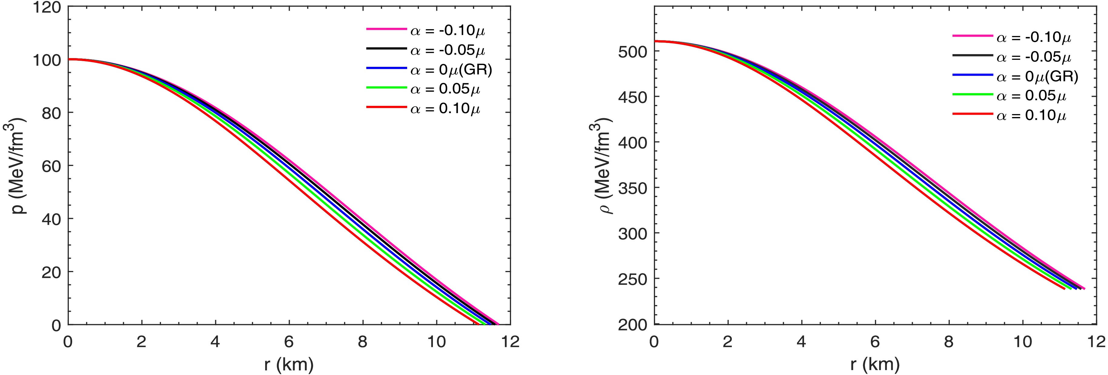
Figure 1.  (color online) Variation of the pressure $ p(r) $(left panel) and energy density versus radius r with a set of parameters as $ B=70 $ MeV/fm³, $ \Delta=100 $ MeV, $ m_{s}=100 $ MeV, and $ \rho_{c}=510 $ MeV/fm³.

The structure of quark stars is unique compared to other compact objects such as white dwarfs and neutron stars. Fig. 2-5 illustrate the mass-energy density and mass-radius relations for quark stars under $ f(R,L_{m},T) $ gravity model. These figures also show the mass constraints of massive compact objects based on recent experimental observations. The red region, with a mass of $ M = 1.97 \pm 0.04M_{\odot} $, represents the mass range constraint from PSR J1614-2230 [33]. The orange region, with a mass range of $ M = 2.08 \pm 0.07M_{\odot} $, corresponds to the data from PSR J0740+6620 [84]. The green region, with $ M = 2.35 \pm 0.17M_{\odot} $, is based on the data from PSR J0952-0607 [85]. The yellow region represents the mass range of the companion object in the gravitational wave event GW190814, with a mass range of $ 2.50-2.67M_{\odot} $ [34]. In Fig. 2, the mass-radius curves of quark stars are shown on the left for different values of the gravitational parameter α, with the parameters set as $ B = 70 $ MeV/fm³, $ m_{s} = $ 100MeV, and Δ =100MeV. The solid blue curve denotes the result from GR, while the other curves correspond to the case of the $ f(R,L_{m},T) $ gravity model, the relevant data are given in Table 1. We find that, compared to neutron stars [32], the structure of CFL quark stars is more sensitive to changes in the parameter α; even small variations in α can lead to significant changes in the mass and radius of quark stars. In the GR case, the quark star has a maximum mass of $ M = 2.09M_{\odot} $ and a radius of $ R = 11.05 $ km, and the mass-radius curve coincides with the data region of the pulsar PSR J0740+6620, which provides a theoretical explanation for the observations. As the value of α increases, both the maximum mass and its corresponding radius decrease. When α = 0.1 μ, a two solar mass compact star cannot be predicted; while when α = -0.1 μ, the quark star reaches a maximum mass of 2.27 $ M_{\odot} $ with a corresponding radius of 11.19 km, which reasonably explains the observations of the pulsar PSR J0952-0607. In addition, the predicted radii corresponding to the observed masses of the four strange star candidates are presented in Table 2.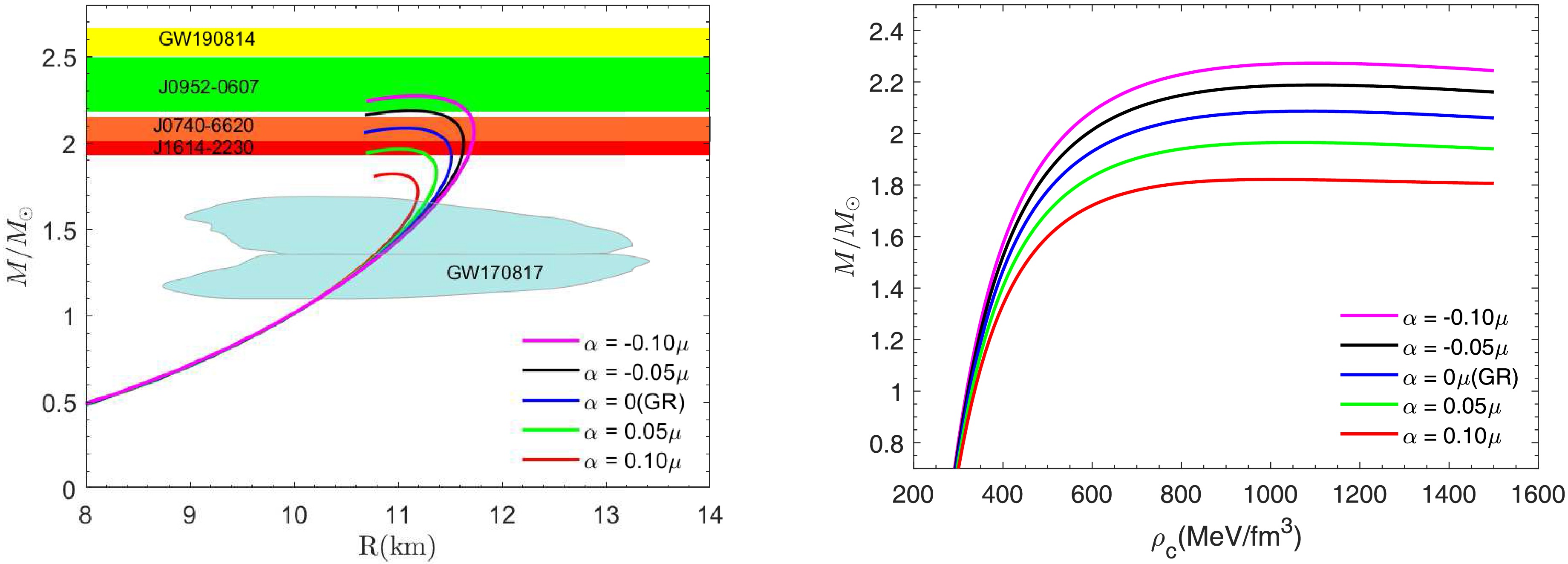

Figure 2.  (color online) The mass-radius curves (left panel) and the mass-central density curves (right panel) for different values of α, with the parameters set as $ B=70 $ MeV/fm³, $ \Delta=100 $ MeV and $ m_{s}=100 $ MeV.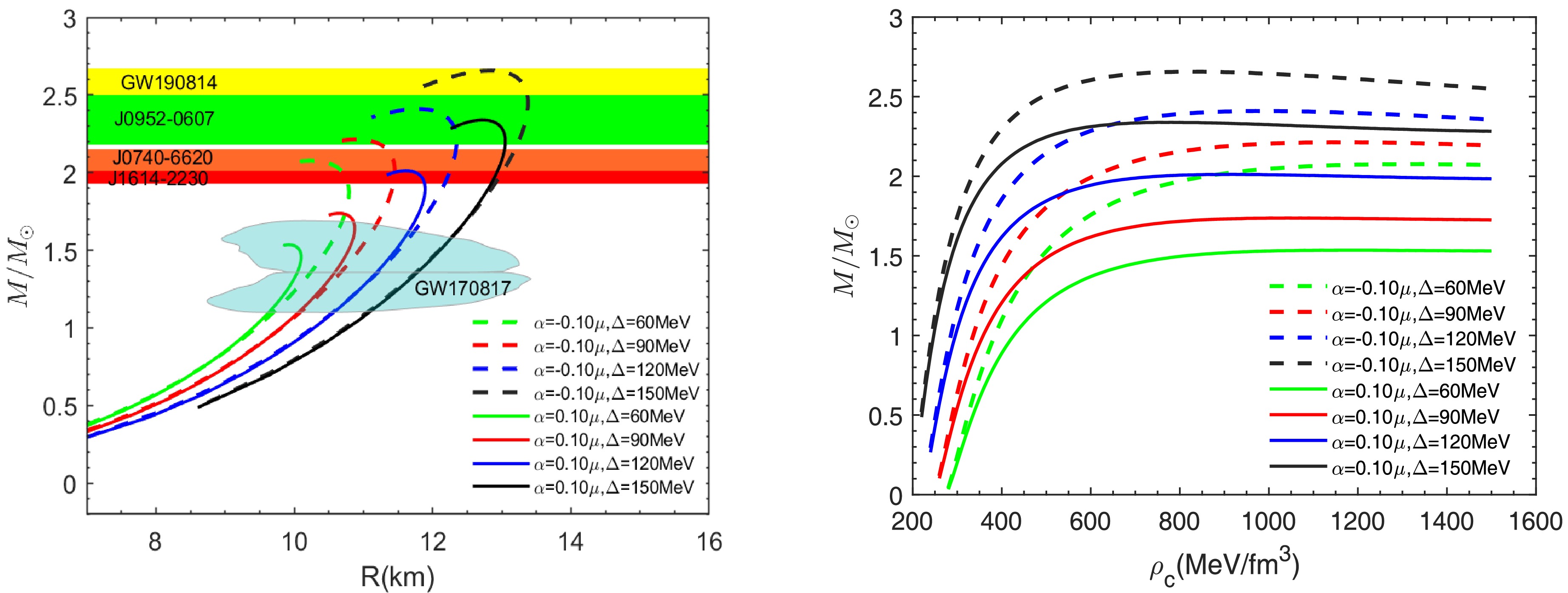

Figure 3.  (color online) The mass-radius curves (left panel) and the mass-central density curves (right panel) for different values of Δ, with the parameters set as $ B=70 $ MeV/fm³ and $ m_{s}=100 $ MeV.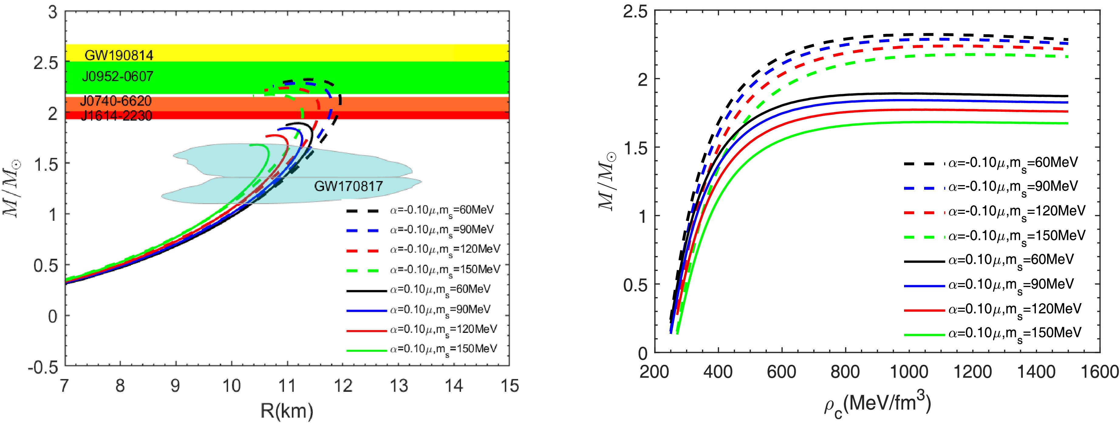

Figure 4.  (color online) The mass-radius curves (left panel) and the mass-central density curves (right panel) for different values of $ m_{s} $, with the parameters set as $ B=70 $ MeV/fm³ and $ \Delta=100 $ MeV.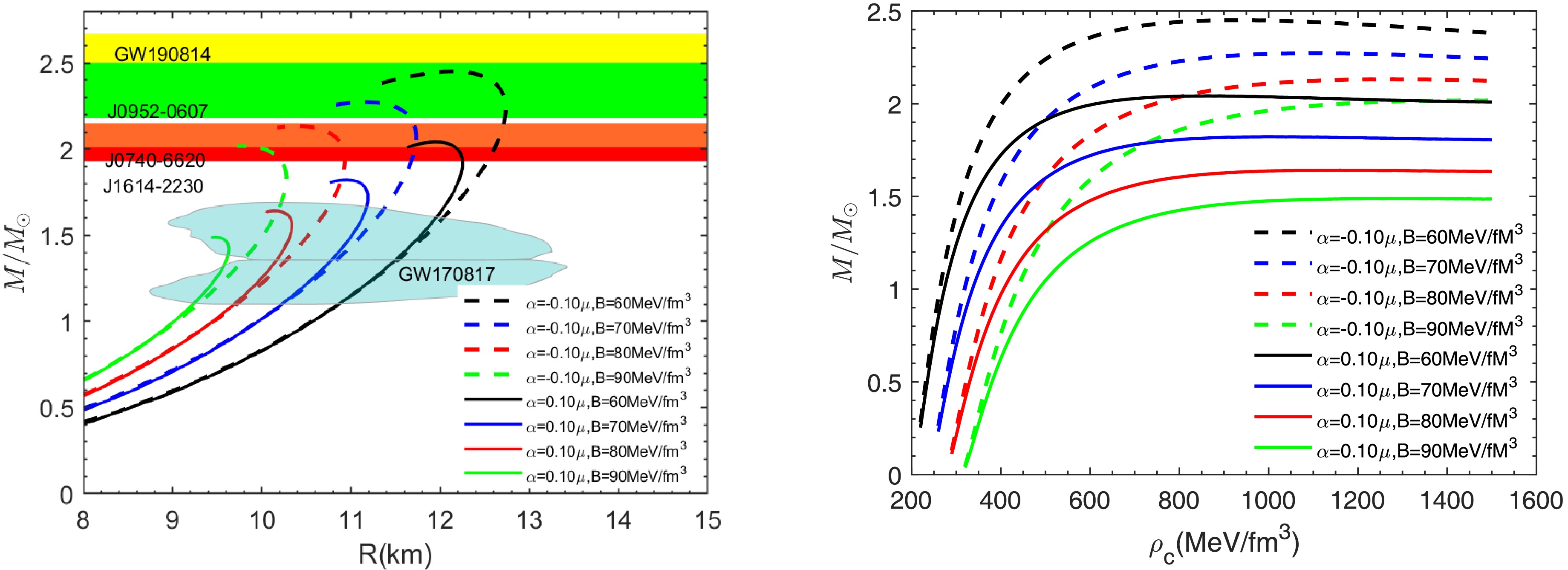

Figure 5.  (color online) The mass-radius curves (left panel) and the mass-central density curves (right panel) for different values of B, with the parameters set as $ \Delta=100 $ MeV and $ m_{s}=100 $ MeV.

α(μ)	$ M_{max} $ $(M_{\odot}) $	R (km)	σ	$ Z_{surf} $	PSR J1614-2230	PSR J0740-6620	PSR J0952-0607	GW190184
-0.10	2.27	11.19	0.57	0.53	$ 11.69^{+0.02}_{-0.02} $	$ 11.72^{+0.00}_{-0.03} $	–	–
-0.05	2.19	11.10	0.55	0.50	$ 11.63^{+0.01}_{-0.02} $	$ 11.60^{+0.04}_{-0.13} $	–	–
0.00	2.09	11.05	0.53	0.46	$ 11.50^{+0.02}_{-0.04} $	$ 11.22^{+0.24}_{-0.17} $	–	–
0.05	1.97	11.00	0.50	0.42	$ 11.00^{+0.28}_{-0.00} $	–	–	–
0.10	1.82	10.96	0.47	0.37	–	–	–	–

Table 1.  Properties of quark stars in $ f(R,L_{m},T) $ gravity corresponding to various selected values of α. Here, $ B=70 $ MeV/fm³, $ \Delta=100 $ MeV and $ m_{s}=100 $ MeV.

α(μ)	Δ (MeV)	$ M_{max} $ $(M_{\odot}) $	R (km)	σ	$ Z_{surf} $	PSR J1614-2230	PSR J0740-6620	PSR J0952-0607	GW190184
	60	2.08	10.20	0.57	0.53	$ 10.75^{+0.03}_{-0.06} $	$ 10.20^{+0.49}_{-0.00} $	–	–
-0.1	90	2.21	10.86	0.57	0.53	$ 10.45^{+0.01}_{-0.01} $	$ 10.44^{+0.00}_{-0.01} $	10.86-11.25	–
	120	2.41	11.81	0.57	0.53	$ 10.22^{+0.05}_{-0.04} $	$ 12.31^{+0.04}_{+} $	$ 12.23^{+0.12}_{-0.42} $	–
	150	2.65	12.85	0.58	0.54	$ 12.97^{+0.05}_{-0.06} $	$ 13.11^{+0.08}_{-0.09} $	$ 13.36^{+0.02}_{-0.13} $	12.85-13.37
	60	1.54	9.91	0.44	0.33	–	–	–	–
0.1	90	1.74	10.65	0.46	0.36	–	–	–	–
	120	2.01	11.61	0.48	0.39	$ 10.85^{+0.04}_{-0.24} $	10.61	–	–
	150	2.34	12.72	0.52	0.44	$ 12.90^{+0.04}_{-0.05} $	$ 13.00^{+0.04}_{-0.06} $	12.75-13.05	–

Table 2.  Properties of quark stars in $ f(R,L_{m},T) $ gravity corresponding to various selected values of Δ. Here, $ B=70 $ MeV/fm³ and $ m_{s}=100 $ MeV.

Next, we investigate the effect of Δ on the structure of quark stars. In Fig. 3, we analyze the $ M-R $ and $ M-\rho_{c} $ relations of quark stars as Δ varies. The dashed and solid lines correspond to the cases of $ \alpha = -0.1 $ μ and $ \alpha = 0.1 $ μ, respectively, and the other parameters are set to B = 70MeV/fm³ and $ m_{s} $ = 100MeV. Table 2 shows some quantities related to the properties of quark stars. As Δ increases from 60MeV to 120MeV, the maximum mass increases gradually. This is because the decrease in Δ leads to a softening of the equation of state, which reduces the star's ability to support its own gravity. For the case $ \alpha = 0.1 $ μ, the maximum mass ranges from 1.54 to 2.34 $ M_{\odot} $. Remarkably, when $ \alpha = -0.1 $ μ and Δ = 120MeV, the maximum mass increases to 2.65 $ M_{\odot} $, which corresponds to a radius of 12.85km. At this point, the mass-radius curve passes exactly through the contour of GW190814. Therefore, it can also be inferred from the figure that the stiffer equation of state is able to fit the observations of GW190814 after the Δ exceeds 120MeV. We then proceed to study the impact of $ m_{s} $ on the structure of quark stars. Fig. 4 presents the results for α varying within the range $ [-0.8, 1.0] $, while other parameters are held constant at Δ = 100 MeV and $ B = 70 $ MeV/fm³. From the figure, it is evident that as $ m_{s} $ increases from 100 to 150 MeV, the equation of state softens, leading to a slight decrease in the maximum mass of the quark star. For the case of $ \alpha = 0.1 $ μ, the maximum mass of the quark star is 1.89 $ M_{\odot} $, which is not consistent with observations of massive pulsars. When $ \alpha = -0.1 $ μ, the maximum mass ranges from 2.18 to 2.32 $ M_{\odot} $, with the corresponding radius ranging from 9.82 to 12.21 km, as shown in Table 3.

α(μ)	$ m_{s} $(MeV)	$ M_{max} $ $(M_{\odot}) $	R (km)	σ	$ Z_{surf} $	PSR J1614-2230	PSR J0740-6620	PSR J0952-0607	GW190184
	60	2.32	11.38	0.57	0.53	$ 11.90^{+0.03}_{-0.03} $	$ 11.96^{+0.00}_{-0.03} $	11.38-11.94	–
-0.1	90	2.28	11.25	0.57	0.53	$ 11.76^{+0.03}_{-0.02} $	$ 11.80^{+0.00}_{-0.01} $	11.25-11.76	–
	120	2.23	11.07	0.56	0.52	$ 11.56^{+0.01}_{-0.02} $	$ 11.57^{+0.00}_{-0.06} $	11.07-11.45	–
	150	2.18	10.84	0.56	0.52	$ 11.28^{+0.00}_{-0.01} $	$ 11.22^{+0.06}_{-0.16} $	10.84	–
	60	1.89	11.20	0.47	0.37	–	–	–	–
0.1	90	1.84	11.03	0.46	0.37	–	–	–	–
	120	1.77	10.79	0.46	0.36	–	–	–	–
	150	1.68	10.45	0.45	0.35	–	–	–	–

Table 3.  Properties of quark stars in $ f(R,L_{m},T) $ gravity corresponding to various selected values of $ m_{s} $. Here, $ B=70 $ MeV/fm³ and $ \Delta=100 $ MeV.

Finally, on the left side of Fig. 5, we investigate the effect of the B, which varies in the range of $ 60-90 $ MeV/fm³, on the mass-radius relation of quark stars. The other parameters are set as $ m_{s} $ = 150MeV and Δ = 100MeV. The results show that as the value of B decreases, both the maximum mass and radius of the quark star increase significantly. For the case of $ \alpha = 0.1 $ μ, the maximum mass ranges from 1.49 to 2.04 $ M_{\odot} $, with the corresponding radius ranging from 9.48 to 11.96, as shown in Table 4. When $ \alpha = -0.1 $ μ, the mass-radius curve passes exactly through the contour lines of the data except for GW190814. The shaded regions in Figs. 2-5 represent the mass-radius constraints from the gravitational wave event GW170817, indicating that the compact star models generated by the above parameters all satisfy these constraints. Furthermore, Fig. 6 shows contour plots of the maximum mass and the corresponding radius across the entire range of parameter values, with the 2.00 $ M_{\odot} $ contour explicitly marked. Parameter combinations above this contour are compatible with both the observed massive pulsars and the mass-radius constraints inferred from gravitational wave events GW170817.

α(μ)	B(MeV/fm3)	$ M_{max} $ $(M_{\odot}) $	R (km)	σ	$ Z_{surf} $	PSR J1614-2230	PSR J0740-6620	PSR J0952-0607	GW190184
	60	2.45	12.01	0.57	0.54	$ 12.58^{+0.04}_{-0.05} $	$ 12.68^{+0.04}_{-0.06} $	$ 12.67^{+0.07}_{-0.52} $	–
-0.1	70	2.27	11.19	0.57	0.53	$ 11.69^{+0.02}_{-0.02} $	$ 11.72^{+0.00}_{-0.03} $	–	–
	80	2.13	10.52	0.56	0.52	$ 10.93^{+0.00}_{-0.02} $	$ 10.80^{+0.11}_{-0.53} $	–	–
	90	2.01	9.97	0.56	0.52	$ 10.12^{+0.11}_{-0.33} $	9.78	–	–
	60	2.04	11.96	0.48	0.39	$ 12.23^{+0.02}_{-0.06} $	11.96-12.17	–	–
0.1	70	1.82	10.96	0.47	0.37	–	–	–	–
	80	1.64	10.14	0.46	0.35	–	–	–	–
	90	1.49	9.48	0.44	0.34	–	–	–	–

Table 4.  Properties of quark stars in $ f(R,L_{m},T) $ gravity corresponding to various selected values of B. Here, $ \Delta=100 $ MeV and $ m_{s}=100 $ MeV.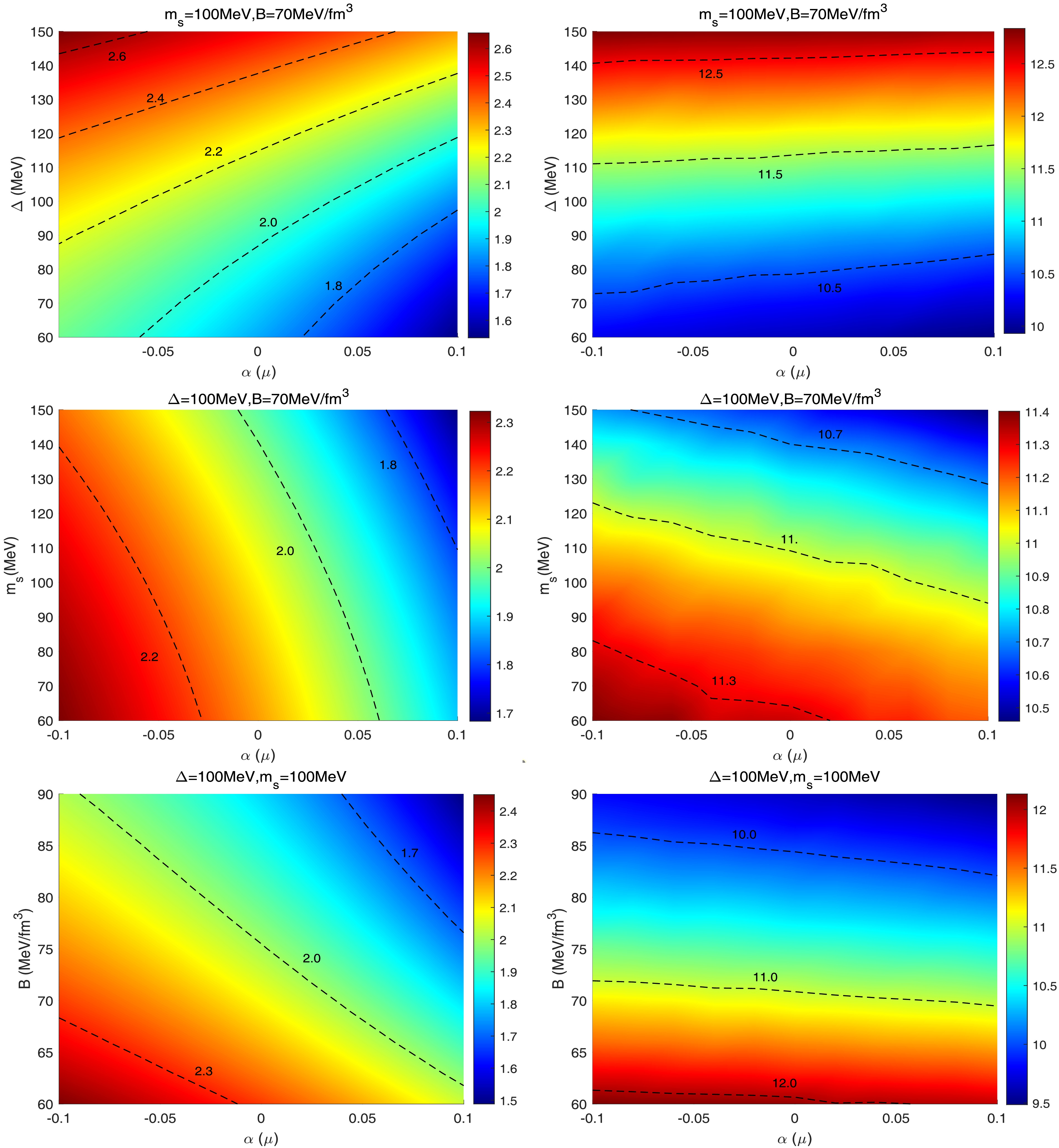

Figure 6.  (color online) The contour plots of the maximum mass (left panel) and the corresponding radius (right panel).

Additionally, the right side of Figs. 2-5 illustrates a plot of mass versus the central energy density, which is numerically calculated in the range $ 400 \leq \rho_{c} \leq 1500 $ MeV/fm³. According to the Harrison-Zeldovich-Novikov criterion [86], the point on each curve that satisfies $ dM/d\rho_{c} = 0 $ is considered to be the critical point at which the star moves from a stable to an unstable state. As can be seen in Fig. 4, the mass of the star increases as the central energy density increases in this range. However, when the central energy density increases to a certain point, the mass of the star begins to decrease. Therefore, there exists a maximum mass value beyond which the star becomes unstable.

Compact objects such as neutron stars, quark stars, and black holes possess extremely strong gravitational fields on their surfaces. When observed from a distant point, the spectral lines emitted by radiation sources within the strong gravitational field will appear redshifted, which is known as gravitational redshift. By measuring the gravitational redshift of compact objects, key physical parameters such as the mass and radius of the stars can be indirectly inferred. These parameters are crucial for understanding the internal structure of the objects. The gravitational redshift at the surface of a star is usually denoted by $ Z_{surf} $, and its expression is given by:

where σ denotes the compactness of quark stars. The surface gravitational redshift corresponding to the maximum mass quark star is given in the last column of Tables 1. The gravitational redshift is 0.46 under GR; while it is 0.37 and 0.53 when α takes the values of 0.1 μ and -0.1 μ, respectively. This result indicates that an increase in α leads to a decrease in the gravitational redshift. The influence of equation of state parameters on the gravitational redshift was also studied, with results presented in Tables 2-4. The study shows that the gravitational redshift decreases with increasing $ m_{s} $ and B, while an increase in Δ results in an increase in the gravitational redshift. Moreover, these tables also provide values for the compactness, and we observe that the compactness and gravitational redshift follow the same trend as the model parameters change. Moreover, we find that the effect of α on the gravitational redshift and compactness is significantly stronger than that of the equation of state parameters. Therefore, precise measurements of these two quantities are expected to effectively break the degeneracy between the gravitational parameter and the equation of state parameters.

We examine the stability of stellar configurations by calculating the sound speed, defined as $ V_s^2 = dp/d\rho $. The causality condition requires that the sound speed remain below the speed of light, i.e., $ V_s^2 < 1 $. As shown in Fig. 7, the speeds lie within the acceptable range and vary smoothly across different parameter values. This indicates that the models satisfy the causality condition.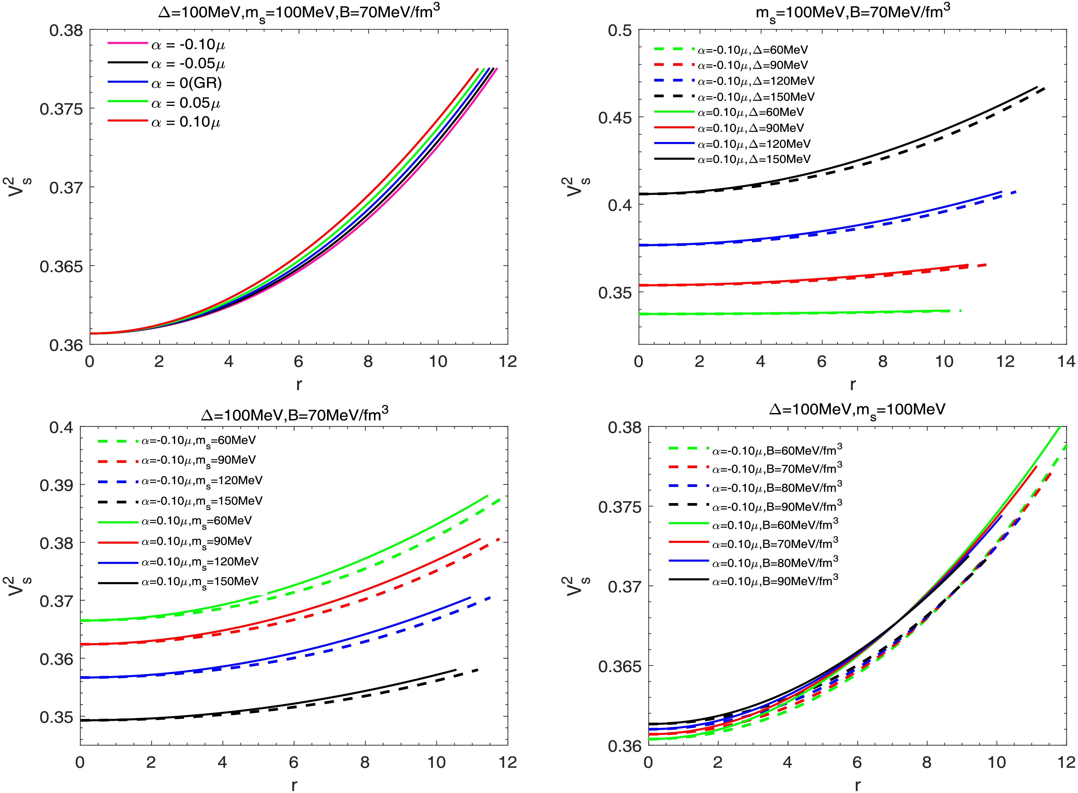

Figure 7.  (color online) Behavior of the sound speed versus radius. Here $ \rho_{c}=510 $ MeV/fm³.

In the quark star model, studying the adiabatic index is an important method for analyzing the stability of the system. Chandrasekhar was the first to use the variational method to propose a theory for describing the dynamical stability of relativistic star systems under infinitesimal radial adiabatic disturbances. For adiabatic perturbations, the relationship between the adiabatic index and the speed of sound is crucial, and it is defined as:

According to the study by Heintzmann and Hillebrandt [87], due to relativistic effects, the instability of the system leads to a critical adiabatic index Γ higher than the Newtonian value $ \Gamma=4/3 $. The behavior of the adiabatic index as a function of radius is discussed, and as shown in Fig. 8, the adiabatic index satisfies $ \Gamma > 4/3 $ for different values of the parameters. This indicates that the model constructed under $ f(R,L_{m},T) $ gravity framework is stable against radial adiabatic infinitesimal perturbations.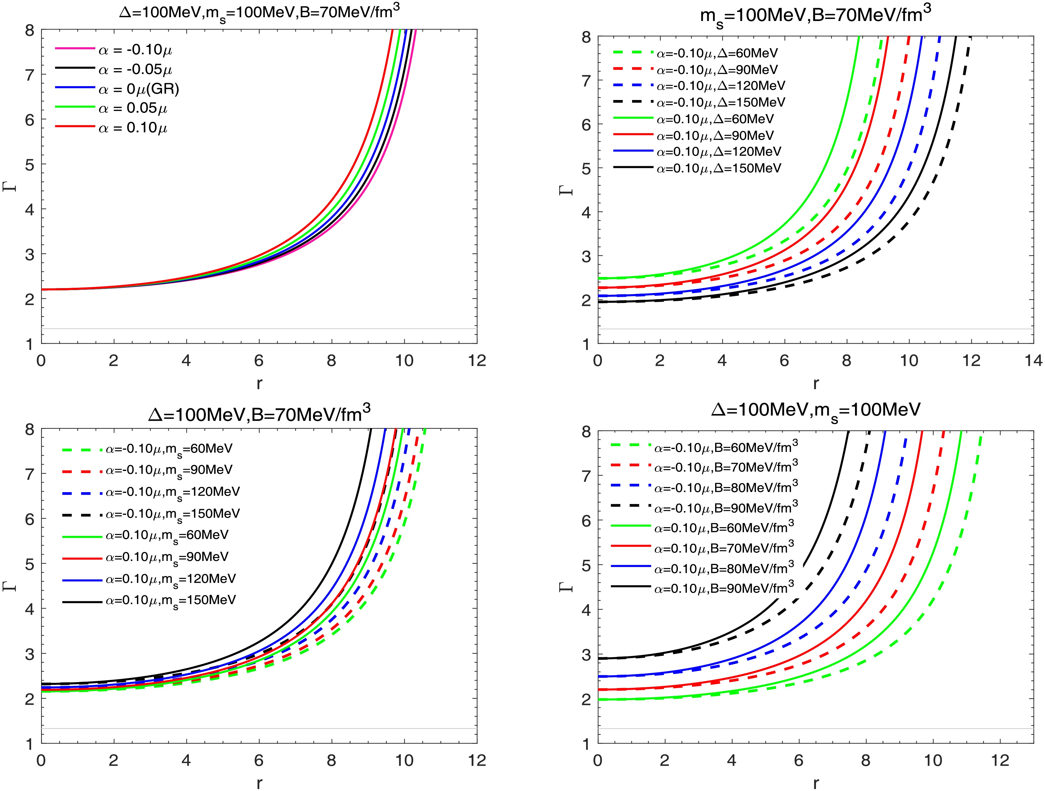

Figure 8.  (color online) Behavior of adiabatic index versus radius. Here $ \rho_{c}=510 $ MeV/fm³.

In this paper, we systematically study the structural properties of CFL quark stars in $ f(R,L_{m},T) $ gravity, utilizing observational data of massive pulsars. We first investigate the impact of the gravitational parameter α on the mass-radius relation of quark stars. The results indicate that, within the $ f(R,L_{m},T) $ gravity model, both the maximum mass and the corresponding radius of the quark star are highly sensitive to variations in α. Specifically, the maximum mass decreases as the α increases, and the mass-radius curve aligns well with observational data from massive pulsars and gravitational wave events. For example, when $ B = 70 $ MeV/fm³, $ m_{s} = 100 $ MeV, and $ \Delta= 100 $ MeV, the maximum mass reaches 2.27 $ M_{\odot} $ as α decreases to -0.1 μ. We further explore the effect of the equation of state parameters on the mass-radius relation. An increase in Δ stiffens the equation of state, leading to an increase in the maximum mass of the quark star, whereas an increase in $ m_{s} $ produces the opposite effect. The bag constant B also influences the mass-radius relation, with both the maximum mass and radius increasing as B decreases.

In addition, we analyzed the compactness and gravitational redshift of quark stars. The results show that both the compactness and gravitational redshift decrease as the parameter α increases, and they also change with variations in the equation of state parameters. Finally,we further examined the adiabatic index Γ, which is used to assess the stability of the quark star model. The study shows that under the $ f(R,L_{m},T) $ gravity model, the adiabatic index is always greater than the Newtonian value, indicating that the model is stable against radial adiabatic perturbations.