Predictions of unknown masses in the feedforward neural network

Atomic mass (or mass for short) is one of the fundamental quantities of a nucleus. Atomic mass data are crucial in nuclear physics, astrophysics, and nuclear technology [1, 2]. They reveal the interaction mechanisms between nucleons, including strong interactions, weak interactions, and electromagnetic interactions [3], as well as the resulting shell effects [4, 5] and deformations [6, 7]. Although significant advances have been made in the measurement of mass [8−11], the mass of many unstable nuclei far from the β-stability line is unknown, such as most nuclei involved in the rapid neutron capture process (r-process) and many short-lived neutron-rich radioactive nuclei [12, 13].

Mass prediction has been one of the hot topics in nuclear structure theory. Generally speaking, theoretical mass models can be divided into global type and local type. Global mass models describe masses by considering the macroscopic and/or microscopic properties of the nucleus, such as the liquid drop model (LDM) [14], the Bethe-Weizsäcker (BW) model [15, 16], the relativistic mean-field (RMF) model [17−19], the Duflo-Zuker (DZ) model [20], the finite-range droplet model (FRDM) [21], the Skyrme-Hartree-Fock-Bogoliubov (SHFB) theory [22−24], the modified Weizsäcker-Skyrme (WS) mass formula [25−28], and so on. Local mass models are characterized by having fewer model parameters and simpler calculations, allowing them to accurately describe and predict the masses of nuclei near the β-stability line, such as the Audi-Wasptra extrapolation [8−11], the Garvey-Kelson (GK) mass relation [29−31], the generalized GK mass relations (GKS) [32], the improved Jänecke mass formula (GK+J) [33], and the mass relations based on proton-neutron interactions [34, 35]. For a comprehensive review, see Ref. [36].

Using the Machine Learning (ML) to analyze and predict nuclear data is one of the focuses in the field of nuclear physics, which is helpful to further understand the nuclear structure and reaction mechanism [37−40]. In the literature, neural networks have made significant progress in optimizing global mass models [41−54], as well as predicting α-decay half-life [55], level density [56], charge density [57], and so on. For example, the feedforward neural network (FNN) reduced the root-mean-square deviations (RMSD) of the LDM from 2.38 MeV to 196 keV using multiple hidden layers [41]. The Bayesian neural network (BNN) was performed to improve the nuclear mass predictions of six global mass models and better predictive performance can be achieved if more physical features are included [43]. By combining the global nuclear mass model and local features, the convolutional neural network (CNN) achieved good optimization results in both training sets and extrapolating new masses [47]. Because the RMSD of local mass models are low (mostly tens to hundreds of keV), there is little research on the optimization of local mass model by neural network. We note that back-propagation (BP) neural network was applied to improve the local mass relations which connect with the proton-neutron interactions for nuclei with $ A\geqslant 100 $ [58]. Although the improvement to the local mass model is modest, it has the advantage that there is no increase in RMSD in a larger mass region [58].

The purpose of this paper is to improve the local mass models of GK, GKs and GK+J within the framework of the feedforward neural network (FNN). Among various machine learning methods, the FNN has the advantages of simple architecture, strong ability to handle low-dimensional inputs and non-spatial features, high interpretability, and powerful function approximation capability [41, 42, 55, 56, 59, 60]. Therefore, the FNN is selected to optimize the local mass models in this paper. By carefully designing the input layer, hidden layer and output layer of the FNN, the prediction accuracy of the three models has been significantly improved. For known masses in AME2012, the RMSD from experimental values of GK, GKS, and GK+J are reduced by $ 11 $ keV, $ 32 $ keV, and $ 623 $ keV, respectively. For the new masses from AME2012 to AME2020, the RMSD reduction for the three models is $ 44 $ keV, $ 20 $ keV and $ 963 $ keV, respectively.

This paper is organized as follows. In Sec. 2, a brief introduction to the FNN is given. In Sec. 3, four neural network structures are designed and the optimal network structure of three local mass models is discussed. Our improvements in both descriptions and predictions of mass excess are investigated. In Sec. 4, one/two-proton/neutron separation energies ($ S_p,S_{2p} $,$ S_n,S_{2n} $), and α-decay energies $ Q_\alpha $ are investigated. In particular, the α-decay energy of nuclei with proton number Z from 82 to 108 and its odd-even staggering (OES) are discussed. The summary and conclusions are given in Sec. 5.

Neural network is a type of computational model that emulate the operational principles of the human brain, consisting of multiple layers of nodes (neurons), which typically include an input layer, hidden layers, and an output layer. Each neuron receives input signals from the previous layer, applies an activation function after weighted summation, generates output signals and passes them to the next layer.

The FNN neural network constructed in this paper contains an input layer, one hidden layer, and an output layer. The activation function is chosen to be the hyperbolic tangent function. Let $ x = \{x_i\} $ be the input of the neural network, $ h_j $ be the output value of the hidden layer node j, and $ \hat{y} $ be the output of the neural network. Then, we have [60]

with

Here, $ w = \{a, b_j, w^{(2)}_{j}, w^{(1)}_{ji}\} $ denotes the neural network parameter. a is a constant term that helps to adjust the output layer's prediction; $ b_j $ is the bias term for the hidden layer neurons, which is used to adjust the activation values; $ w^{(1)}_{ji} $ and $ w^{(2)}_{j} $ are the weight matrices representing the connections from the input layer to the hidden layer and from the hidden layer to the output layer, respectively, and determine the strength of the connections between layers. H and I refer to the number of hidden layer neurons and inputs, respectively. During the initialization process of the parameter w, a and $ b_j $ are set as zero vectors, $ w^{(1)}_{ji} $ and $ w^{(2)}_{j} $ are generated through Xavier initialization based on a normal distribution. To ensure reproducibility of the results, a random seed strategy is adopted to keep the weight matrices generated during each initialization consistent.

Given a training set $ P = \{(x_i, y_i) \mid i \in \{1, 2, \ldots, {\cal{N}}\}\} $ consisting of $ {\cal{N}} $ data points and a loss function, the parameters w of the neural network can be trained. For a neural network regression prediction problem, the RMSD function is typically chosen as the loss function, which is defined as follows.

The neural network optimizes the parameter w by minimizing the value of the loss function, learning to reduce the gap between the predicted values and the actual values to improve prediction accuracy. Here, the Adam algorithm [61] is adopted to optimize the neural network. It effectively improves the training efficiency and performance of the neural network by avoiding gradient issues, accelerating convergence, and utilizing prior knowledge to enhance model performance. During the training process, a back-propagation algorithm is used to calculate the error and propagate the error from the output layer back to the hidden and input layers layer by layer, gradually adjusting the weights to optimize the performance of the network.

In order to study the description and prediction of mass excess in different neural networks, four neural network structures are designed. Since the neural network with a single hidden layer is easier to understand, more economical in terms of computational resources, and also reduces the risk of overfitting, a single hidden layer neural network is adopted. Specific structural parameters, including input variables, number of hidden layer neurons H, output, and the total number of neural network parameters w (denoted by $ \mathbb{N} $) are presented in Table 1. The H values of the four structures are changed to ensure that total number of parameters in the neural network is consistent. Here, N and Z represent the neutron and proton numbers, respectively. $ P = N_{\rm p} N_{\rm n}/(N_{\rm p} + N_{\rm n}) $ with the valence proton number $ N_{\rm p} $ and valence neutron number $ N_{\rm n} $ is the average number of interactions of each valence nucleon with those of the other type, which is a useful indicator of the pairing versus p-n competition [62]. $ Z_{\text{eo}} $ and $ N_{\text{eo}} $ are related to the pairing effect. If Z (N) is even, $ Z_{\text{eo}} $ ($ N_{\text{eo}} $) equals to 1; otherwise, they equal to zero. $ N_{\text{shell}} $ and $ Z_{\text{shell}} $ represent the shell model orbitals of the last proton and neutron [63], associated with the shell effects. The values of $ N_{\text{shell}} $ and $ Z_{\text{shell}} $ are defined as 1, 2, 3, 4, or 5, depending on whether the proton or neutron number falls within the specified ranges $ [8, 28] $, $ [29, 50] $, $ [51, 82] $, $ [83,126] $, and $ [127,184] $, respectively. The output is $ \Delta M = M^{\text{expt}} - M^{\text{th}} $, that is, the deviation between the experimental data and the theoretical prediction of mass excess.

Structure	Input Variables	H	Output	$ \mathbb{N} $
A	$ N, Z $	30	$ \Delta M $	121
B	$ N, Z, P $	24	$ \Delta M $	121
C	$ N, Z, N_{\text{eo}}, Z_{\text{eo}} $	20	$ \Delta M $	121
D	$ N, Z, N_{\text{shell}}, Z_{\text{shell}} $	20	$ \Delta M $	121

Table 1.  Input variables, number of hidden layer neurons H, output, and total number of parameters $ \mathbb{N} $ in four neural network structures. Here, one hidden layer is used.

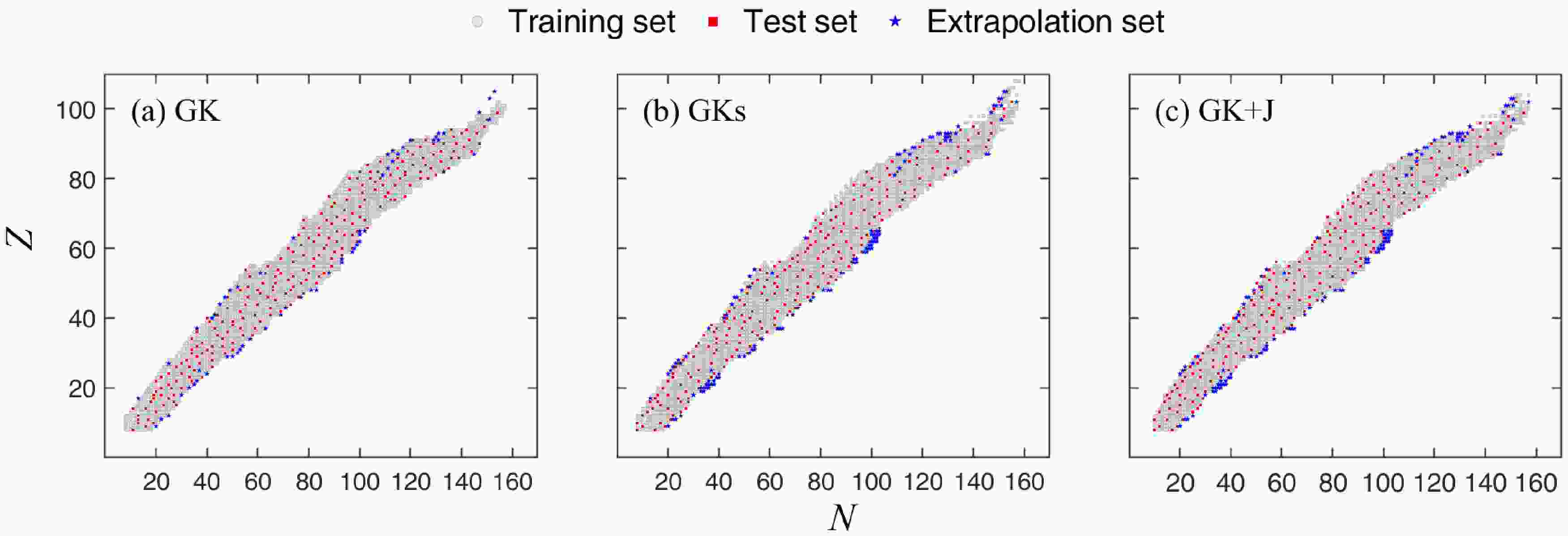
The neural network is trained based on the AME2012 experimental database, for nuclei with $ N\geqslant 8 $ and $ Z\geqslant 8 $. The distribution of the training set and the test set on the nuclear chart is presented in Fig. 1. Here, the ratio of the number of known masses contained in the training set to the test set is $ 9:1 $. The partitioning of these two data sets is random, but it is required that the data cover all regions of the nuclear chart. The nuclei in the test set are distributed both at the edges and within the interior of the nuclear chart, which guarantees the effectiveness and reliability of the testing process. Since the number of known masses in AME2012 described by GK, GKs and GK+J models is 2265, 2318 and 2310 respectively, the training sets and test sets of the three models are not completely consistent, but they all meet the requirement of $ 9:1 $. The sum of the test set and the training set is called the full dataset. To evaluate the extrapolation capability of the neural network, one extrapolation set (denoted by "12-20") is constructed based on the AME2020, including experimental masses that appear in AME2020 but are absent in AME2012. Since the vast majority of nuclei in the extrapolation set spanning from AME2012 to AME2016 are already contained in the 12-20 dataset, only one 12-20 extrapolation set is constructed in this paper. We also experiment with partitioning ratios of $ 7:3 $ and $ 8:2 $. The results indicate that while different ratios yield similar RMSDs on the training and test sets, the $ 9:1 $ ratio performs optimally on the extrapolation. Because the nuclei in the extrapolation set are mainly distributed at the edge of the nuclear chart, the performance of extrapolation is related to the distribution of the training set in the boundary region. Compared with $ 7:3 $ and $ 8:2 $, the $ 9:1 $ ratio makes the training set contain more edge samples, which can help the model learn the boundary behavior better, thus strengthening the extrapolation ability.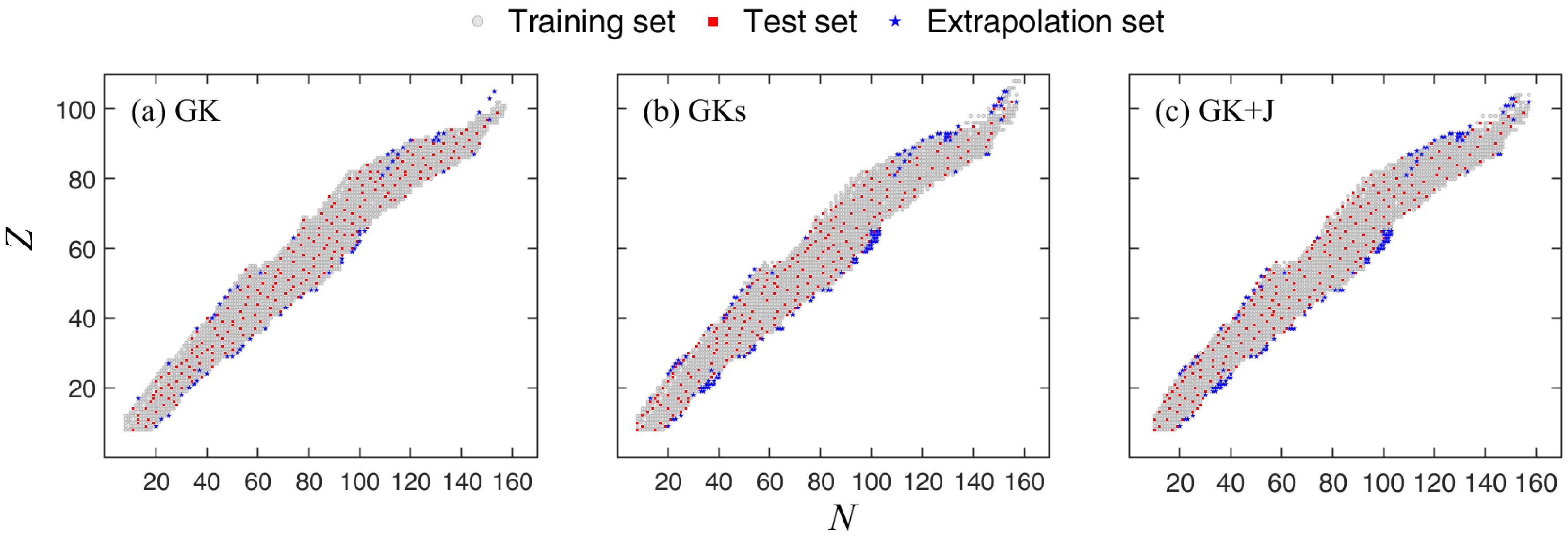

Figure 1.  (Color online) The training set, test set, and extrapolation set on the nuclear chart for the GK, GKs, and GK+J models.

The steps to predict mass excess with the FNN are as follows. Firstly, we construct a neural network using the training set. The input variables are shown in Table 1. The output of the neural network is uniformly given by $ \Delta M (N, Z)= M^{\text{expt}}(N, Z) - M_0^{\text{th}}(N, Z) $. Here, $ M_0^{\text{th}} $ represents the theoretical predicted values of local mass model. Secondly, the optimal hyperparameters are determined through a grid-based parameter tuning process. For the GK, GKs, and GK+J models, the learning rates are set to $ 0.0094 $, $ 0.0095 $, and $ 0.0115 $ respectively, with corresponding training iteration counts of $ 50000 $, $ 60000 $, and $ 50000 $. Thirdly, once the input, output, and hyperparameters are determined, neural network parameters $ w = \{a, b_j, w^{(2)}_{j}, w^{(1)}_{ji}\} $ can be obtained by using Eq. (1). Finally, the predicted deviation $ \Delta M'(N, Z) $ of mass excess by the FNN is reconstructed by Eq. (1). And the predicted value of the FNN is expressed as $ M^{\text{th}}_{\text{FNN}}(N, Z) = \Delta M' (N, Z)+ M_0^{\text{th}}(N, Z) $.

The performance of four neural network structures in predicting nuclear masses are evaluated on the training set, test set, and the full dataset for three local mass models, as shown in Fig. 2. Here, $ \sigma_0 $ and σ represent the mass RMSD between theory and experiment initially and after FNN training, respectively. If the ratio $ \sigma/{\sigma_0} $ is less than 1, it indicates that the prediction of the theoretical model has improved after FNN training. One sees that based on the known masses in the AME2012, the FNN neural network performs optimally with the C structure for the GK, GKs and GK+J models. Furthermore, Fig. 3 shows the extrapolation of these neural networks over the mass from AME2012 to AME2020, where the optimal network structure coincides with those identified in Fig. 2. This indicates that the pairing effect is the most effective correction in improving the GK, GKs and GK+J models. It is known that the GK mass relations are constructed in such a way that the neutron-neutron, proton-proton, and neutron-proton interactions are canceled at the first order. In fact, the GK mass relations are not strictly zero. In the literature [34, 64], it has been found that for different parity combinations of neutrons and protons, the GK relations have an odd-even staggering pattern with respect to the average deviation from zero, which is dominantly originated from the pairing interaction. Therefore, the result that the"pairing effect" as the physical input is the optimal network structure is consistent with the above conclusion.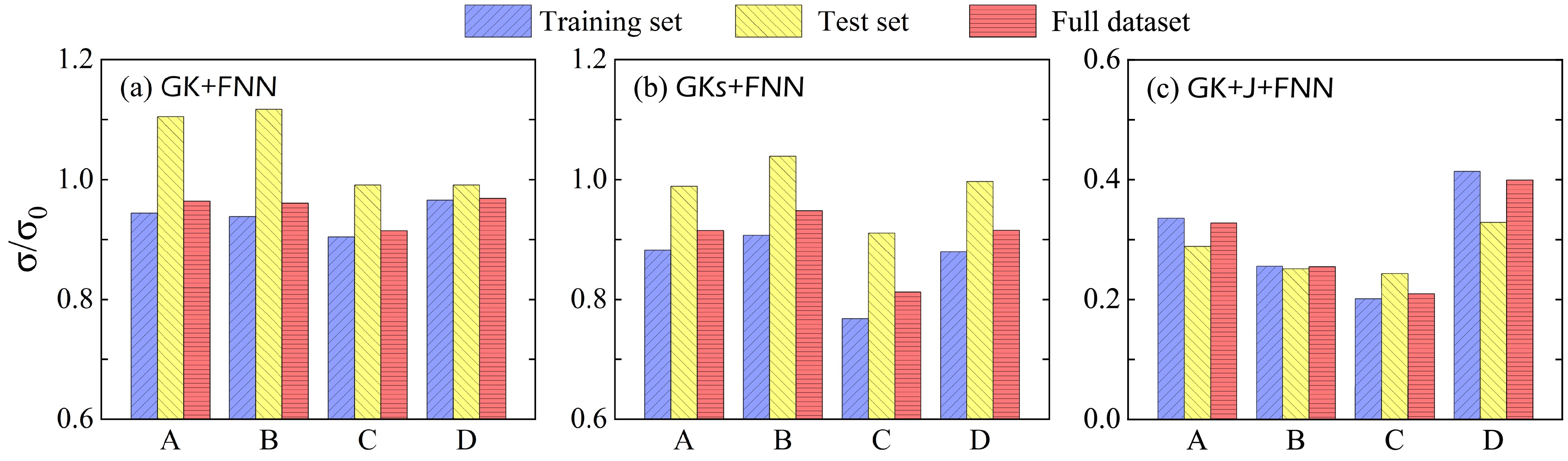

Figure 2.  (Color online) Mass RMSD ratios $ (\sigma / \sigma_0) $ of four network structures of local mass model GK, GKs, and GK+J. Results of the training set, test set, and full dataset are presented by blue, yellow and red, respectively.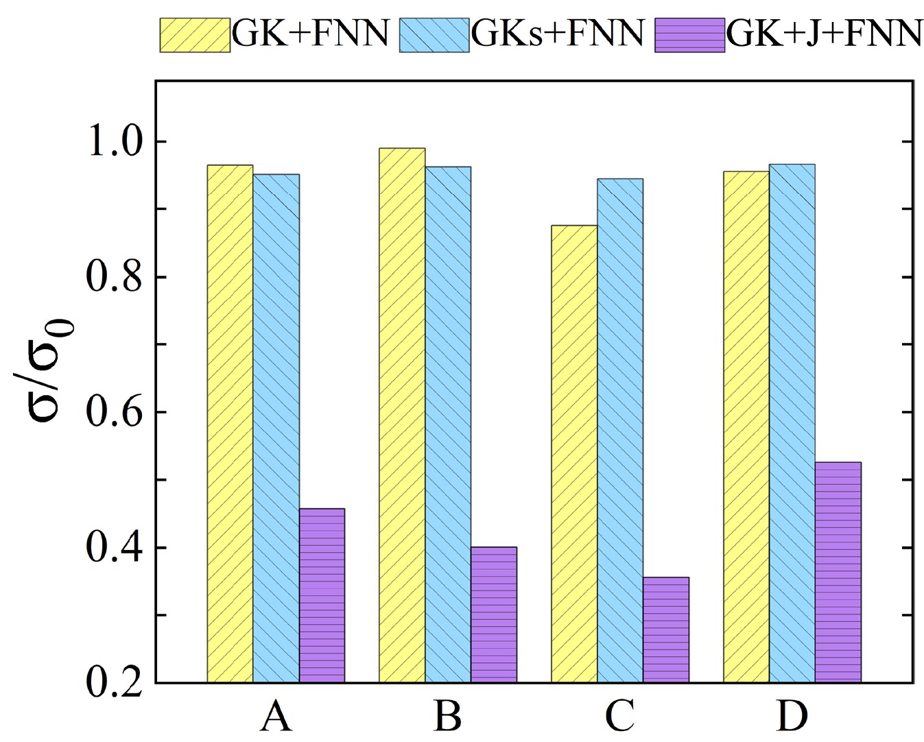

Figure 3.  (Color online) Same as Fig. 2 except for the extrapolation set from AME2012 to AME2020.

Table 2 shows mass RMSDs of the three local mass models under the network structure C for the training set, test set, and full set in AME2012, as well as the results of extrapolation set from AME2012 to AME2020 (denoted by "12-20"). Here, $ \Delta=\sigma_{0}-\sigma $ represents the improvement of the RMSD after FNN training. $ {\cal{N}} $ is the number of nuclei in the corresponding dataset. One sees that, for the known nuclei in AME2012, the RMSD of full dataset is reduced by 11, 32, and 623 keV for the GK, GKs, and GK+J, respectively; for the extrapolation set from AME2012 to AME2020, $ \Delta= $ 44, 20, and 963 keV, respectively. These results demonstrate that the FNN can significantly improve the prediction accuracy of local mass models. For the GK model, the improvement achieved by the FNN on the test set is minor ($ \Delta=2 $ keV). We have experimented with altering the division between the training set and the test set. Although this adjustment can appropriately increase the improvement on the test set, the optimal improvement for the full dataset remains at around 11 keV, and the extrapolation performance is inferior to the existing results. As can be seen from Table 2 (and Fig. 4 below), the original predictive accuracy of the GK model is already quite high, with a RMSD of 142 keV on the test set. Achieving an overall improvement of 11 keV based on such a precise dataset is our current best result. To further validate our results, we replace the mass values in the AME2012 full dataset with the updated values from AME2020 and recalculate the RMSDs in Table 2. The obtained improvements Δ by the FNN for the three models are very close to those in Table 2. This indicates that the optimization effect of the FNN is almost unaffected by the version update of experimental data.

Data	GK+FNN					GKs+FNN					GK+J+FNN
	Train	Test	Full	12-20		Train	Test	Full	12-20		Train	Test	Full	12-20
$ \sigma_0 $	131	142	132	355		154	300	174	348		750	1073	788	1496
σ	118	140	121	311		118	274	142	328		151	261	165	533
Δ	13	2	11	44		36	26	32	20		599	812	623	963
$ {\cal{N}} $	2039	226	2265	61		2087	231	2318	118		2079	231	2310	113

Table 2.  Mass RMSDs (in keV) of the GK, GKs, and GK+J in the neural network structure C for the training set, test set, and full set in AME2012, and extrapolation set from AME2012 to AME2020 (denoted by "12-20"). Here, $ \sigma_0 $ and σ represent the RMSD between theory and experiment initially and after FNN training, respectively. $ \Delta=\sigma_{0}-\sigma $. $ {\cal{N}} $ is the number of nuclei in the corresponding dataset.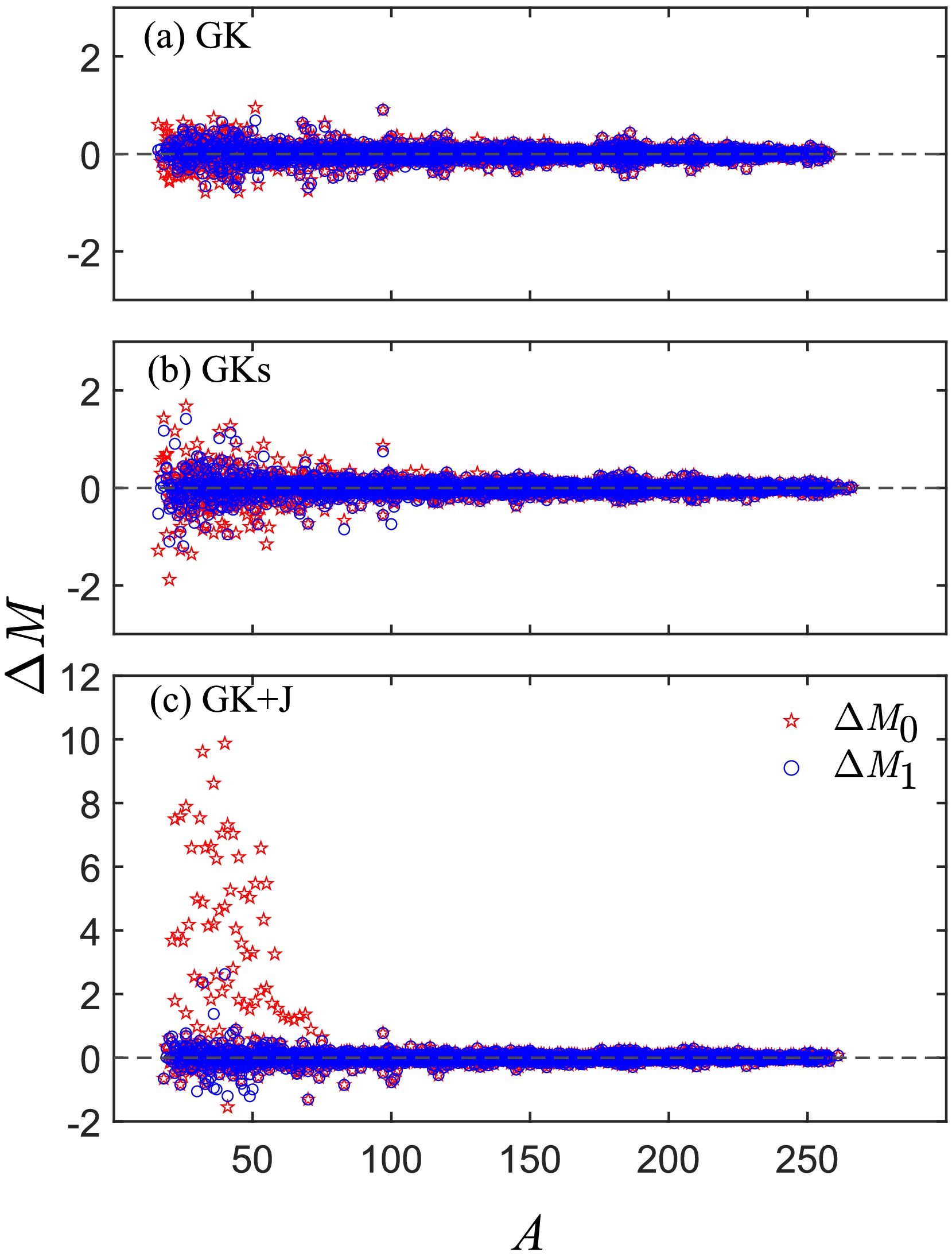

Figure 4.  (Color online) Mass deviation $ \Delta M $ (in MeV) of the GK, GKs and GK+J models in the full dataset of AME2012. Here, $ \Delta M_0 = M^{\text{expt}} - M^{\text{th}}_0 $ represents the deviation of the model itself; $ \Delta M_{1} = M^{\text{expt}} - M^{\text{th}}_{\text{FNN}} $ refers to the results after the FNN improvement.

To evaluate the performance of the FNN in optimizing local mass models in different mass regions, the RMSDs in light ($ 16 \leqslant A < 60 $), medium ($ 60 \leqslant A < 120 $) and heavy ($ A \geqslant 120 $) mass regions of full dataset in the AME2012 are given in Table 3. The initial mass deviation $ \Delta M_0 = M^{\text{expt}} - M^{\text{th}}_0 $ of the three models and the mass deviation $ \Delta M_{1} = M^{\text{expt}} - M^{\text{th}}_{\text{FNN}} $ after FNN improvement are also shown in Fig. 4. It can be seen that in the light mass region, the FNN greatly improves the three mass models, reducing the RMSD between the predicted and experimental values by 44,108 and 1802 keV, respectively. In the medium and heavy mass regions, because the local mass models themselves perform well (the mean RMSD about $ 151 $ keV in the medium region and about $ 76 $ keV in the heavy region), the improvement of the FNN is not as significant as in the light mass region.

Region	$ \sigma_0 $	σ	Δ	$ {\cal{N}} $
GK+FNN
$ 16 \leqslant A< 60 $	257	213	44	297
$ 60 \leqslant A< 120 $	133	133	0	634
$ A \geqslant 120 $	80	79	2	1334
GKs+FNN
$ 16 \leqslant A< 60 $	414	306	108	300
$ 60 \leqslant A< 120 $	134	131	3	632
$ A \geqslant 120 $	75	74	1	1386
GK+J+FNN
$ 16 \leqslant A< 60 $	2183	381	1802	295
$ 60 \leqslant A< 120 $	185	142	42	636
$ A \geqslant 120 $	73	73	0	1379

Table 3.  Mass RMSDs (in keV) for different mass regions of the AME2012 full dataset. The definitions of $ \sigma_0 $, σ, Δ, and $ {\cal{N}} $ are the same as in Table 2.

Finally, it is worth looking at the accuracy of our predictions for the new measured masses after the AME2020. Since the release of AME2020, the masses of about 100 more atomic nuclei have been measured experimentally. GKs and GK+J models can predict 20 of these [65−75], while GK can predict 7. The mass RMSDs after FNN improvement are shown in Table 4. It can be seen that the improved ability of the FNN is robust and can reduce the predictive RMSD of the three models by 16, 27, and 408 keV, respectively.

Data	GK+FNN	GKs+FNN	GK+J+FNN
$ \sigma_0 $	199	208	770
σ	183	181	362
Δ	16	27	408
$ {\cal{N}} $	7	20	20

Table 4.  Same as Table 2 except for the RMSDs (in keV) for the new measured masses after AME2020.

In Table 5 and Fig. 5, the specific predicted values and corresponding mass deviations $ \Delta M $ of the three models for 20 new masses are respectively presented and compared with the predictions in AME2020. Here, for the same nucleus, the predicted value with the smallest deviation from the experiment is expressed by "FNN-Best" in Table 5. According to Table 5 and Fig. 5, the three local mass models optimized by the FNN exhibit excellent performance in extrapolation. For these 20 nuclei, the RMSD between the predicted and experimental values of AME2020 is 195 keV. Of the three models, the GKs model performs best, with a RMSD of 181 keV between its predicted and experimental values, which is 14 keV lower than that of the AME2020. Further, if the optimal prediction value "FNN-best" is taken, the RMSD between the theoretical and experimental value is reduced to 159 keV.

Nuclei	$ \text{GK+FNN} $	$ \text{GKs+FNN} $	$ \text{GK+J+FNN} $	$ \text{FNN-Best} $	AME2020	Expt.
$ ^{65}\text{Cr} $		−28245	−28993	−28245	−28310	−28208 (45) [65]
$ ^{69}\text{Fe} $	−39424	−39208	−38936	−39424	−39199	−39504 (11) [66]
$ ^{70}\text{Fe} $		−36845	−36855	−36855	−36890	−37053 (12) [66]
$ ^{74}\text{Ni} $	−48712	−48527	−48544	−48527	−48700	−48451 (3.5) [67]
$ ^{75}\text{Ni} $		−44068	−43746	−44068	−44240	−44056 (14.7) [67]
$ ^{60}\text{Ca} $		−40019	−39947	−40019	−39590	−40005 (30) [68]
$ ^{103}\text{Rb} $		−33286	−33716	−33286	−33160	−33049 (32) [68]
$ ^{103}\text{Sr} $		−47237	−47371	−47237	−47280	−47220 (29) [69]
$ ^{104}\text{Sr} $		−43698	−44030	−43698	−43760	−43411 (33) [69]
$ ^{105}\text{Sr} $		−38037	−37970	−37970	−38190	−37886 (44) [69]
$ ^{120}\text{Rh} $	−58870	−58636	−58789	−58636	−58620	−58614 (58) [70]
$ ^{99}\text{In} $	−61410	−61267	−61124	−61410	−61376	−61429 (77) [71]
$ ^{133}\text{In} $	−57403	−57390	−57198	−57403	−57690	−57678 (41) [72]
$ ^{134}\text{In} $		−51390	−51328	−51390	−51970	−51855 (44) [72]
$ ^{152}\text{Ce} $	−58969	−58824	−58806	−58824	−58980	−58878 (23) [73]
$ ^{153}\text{Ce} $		−54764	−54860	−54764	−54910	−54712 (24) [73]
$ ^{154}\text{Ce} $		−52059	−52044	−52059	−52220	−52069 (24) [73]
$ ^{150}\text{Yb} $		−38727	−38738	−38727	−38830	−38635 (44) [74]
$ ^{153}\text{Yb} $	−47209	−47212	−47143	−47143	−47160	−47102 (46) [74]
$ ^{251}\text{No} $		82827	82780	82827	82849	82851 (23) [75]

Table 5.  Theoretical predicted values of the newly measured mass excess. The predictions in AME2020 and experimental values are listed for comparison. Here, for the same nucleus, the value with the smallest deviation from the experimental value in the three models is labeled "FNN-Best".

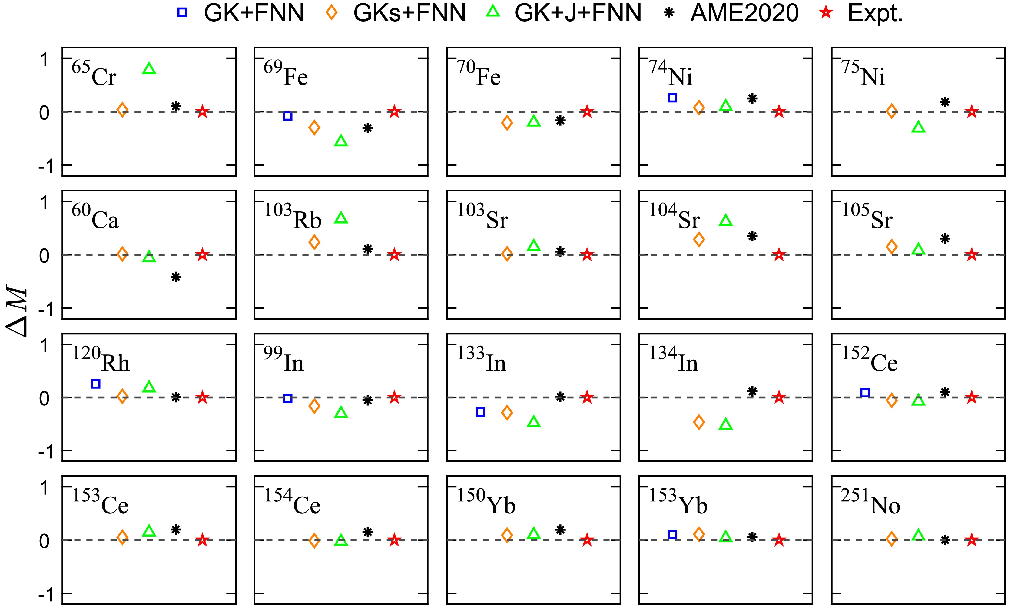
Figure 5.  (Color online) Mass deviation $ \Delta M = M^{\text{expt}} - M^{\text{th}} $ (in MeV) of the GK, GKs and GK+J models for 20 newly measured masses. The AME2020 prediction results are also drawn for comparison.

The mass excess (M) is closely related to various forms of nuclear energy, such as single- and two- proton/neutron separation energies ($ S_p $, $ S_{2p} $, $ S_n $, $ S_{2n} $), and α-decay energy $ Q_\alpha $, defined by

Here, $ S_{ip} $ and $ S_{in} $ represent the i-proton and i-neutron separation energies, respectively.

Using the predicted mass excess, we evaluate the separation energies for single- and two-proton (neutron) emissions, as well as the α-decay energies. The RMSDs between predicted values of three local mass models and the experimental values are listed in Table 6, for nuclei with $ N\geqslant 8 $ and $ Z\geqslant 8 $. Meanwhile, the results of FRDM12 [21] and WS4 [28] are also listed in the table for comparison. Here, the definitions of $ \sigma_0 $, σ, Δ, and $ {\cal{N}} $ are the same as in Table 2. It can be seen that after the optimization of FNN neural network, the three local mass models have been effectively improved. The RMSDs of the five energies of GK, GKs and GK+J are reduced by $ \Delta=12.8 $ keV, 49.8 keV and 265.6 keV on average, respectively. In addition, the prediction accuracy of the three local models improved by FNN is significantly higher than that of FRDM and WS4 models. This indicates that the FNN can effectively improve the local mass models, and our prediction results have certain competitiveness.

Energy	GK+FNN					GKs+FNN					GK+J+FNN					FRDM12			WS4
	$ \sigma_0 $	σ	Δ	$ {\cal{N}} $		$ \sigma_0 $	σ	Δ	$ {\cal{N}} $		$ \sigma_0 $	σ	Δ	$ {\cal{N}} $		$ \sigma_0 $	$ {\cal{N}} $		$ \sigma_0 $	$ {\cal{N}} $
$ S_{n} $	207	188	19	2181		249	198	51	2281		433	226	207	2282		350	2309		257	2309
$ S_{p} $	202	187	15	2147		264	201	63	2252		416	215	201	2254		365	2281		273	2281
$ S_{2n} $	177	168	9	2098		277	212	65	2203		688	233	455	2201		455	2223		266	2223
$ S_{2p} $	192	180	12	2008		292	227	65	2122		683	237	446	2144		470	2134		321	2134
$ Q_\alpha $	213	204	9	2198		188	183	5	2337		223	204	19	2298		552	2342		344	2342

Table 6.  RmsDs (in keV) of single-neutron ($ S_n $), single-proton ($ S_p $), two-neutron ($ S_{2n} $), two-proton ($ S_{2p} $) separation energies, and α-decay energy $ Q_{\alpha} $ with respect to the experimental data in AME2020. Here, the definitions of $ \sigma_0 $, σ, Δ, and $ {\cal{N}} $ are the same as in Table 2.

Next, it is of interest to focus on the α-decay energy of heavy nuclei. The predicted $ Q_{\alpha} $ values for nuclei with proton number Z ranging from 82 to 108 are presented in Fig. 6. Since "GKs+FNN" has the highest prediction accuracy for α-decay energy among the three local models, we only draw the results of GKs+FNN in the figure. Meanwhile, results of the FRDM, WS4 and experimental data are also compared. As shown in the figure, the $ Q_{\alpha} $ values predicted by the GKs+FNN, FRDM and WS4 models are in excellent agreement with the experimental values (with the RMSD 97 keV, 276 keV and 269 keV, respectively). For experimentally unknown nuclei, the three theoretical models (GKs+FNN, FRDM, and WS4) predict roughly the same trend. That is, for nuclei with $ N<126 $, $ Q_{\alpha} $ of each isotopic chain increases as the number of neutrons decreases; for nuclei with $ N>126 $, $ Q_{\alpha} $ decreases as the number of neutrons increases. Notably, for the isotopes with $ Z=82, 84\sim 87 $, the predicted values of the three theoretical models have slightly different trends for the lightest and/or heaviest mass regions.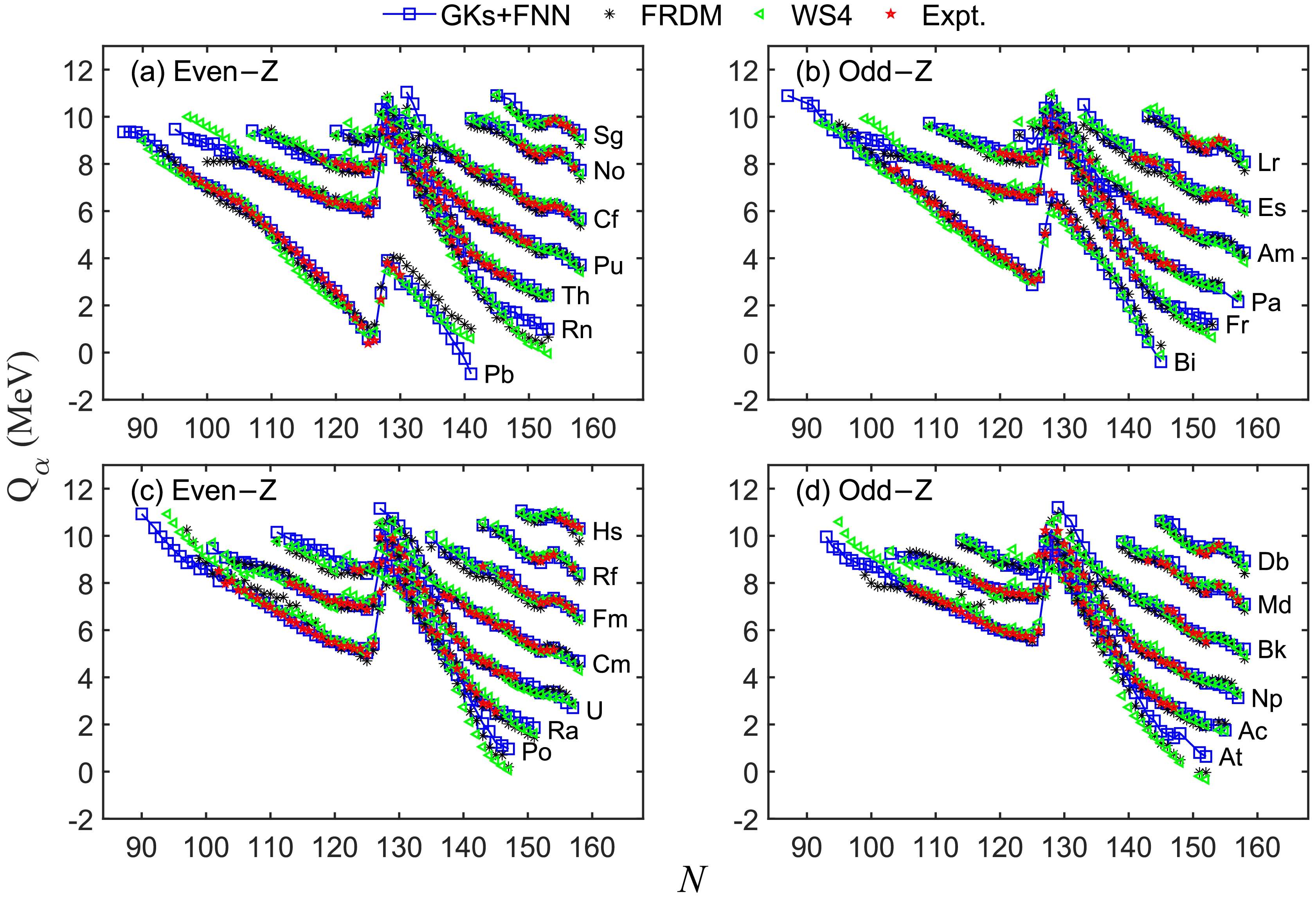

Figure 6.  (Color online) The α-decay energies $ Q_{\alpha} $ (in MeV) for nuclei with proton number Z from 82 to 108. Panels (a,c) and (b,d) refer to the results of even-Z and odd-Z nuclei, respectively. Experimental data are from AME2020.

Recently, an interesting phenomenon has been observed: $ Q_{\alpha} $ energies of nuclei with $ Z > 82 $ and $ N < 126 $ exhibit a distinct odd-even staggering (OES), which is caused by a combination of pairing correlations and blocking effect of unpaired nucleons [76]. The OES of $ Q_{\alpha} $ with the number of neutrons (denoted by $ \Delta Q_{\text{n}} $) or protons (denoted by $ \Delta Q_{\text{p}} $) can be quantitatively studied by the following formula [77−79]:

Our predicted $ \Delta Q_{\text{n}} $ for Rn, Fr, Ra, Ac, Th, Pa, and U isotopes and $ \Delta Q_{\text{p}} $ for $ N=115\sim 125 $ isotones are presented with hollow symbols in Fig. 7 (a) and (b), respectively. The experimental values in the figure are represented by corresponding solid symbols. In order to avoid overlapping, each chain is translated upward by a certain amount, and the value of the translation is shown in the number beside each chain. It can be seen that our results reproduce both neutron OES and proton OES patterns very well. The RMSDs between the theoretical predictions and the experimental values are 51 keV (for 70 known nuclei) in panel (a), and 31 keV (for 62 known nuclei) in panel (b), respectively. In the literature [76], it is pointed out that the typical amplitude of OES for α-decay energy is about 70 keV for nuclei with $ Z>82 $ and $ N<126 $. The mean values of $ |\Delta Q_{\text{n}}| $ and $ |\Delta Q_{\text{p}}| $ predicted by the GKs+FNN are 86 keV and 68 keV, respectively. Our results agree well with the experimental observations.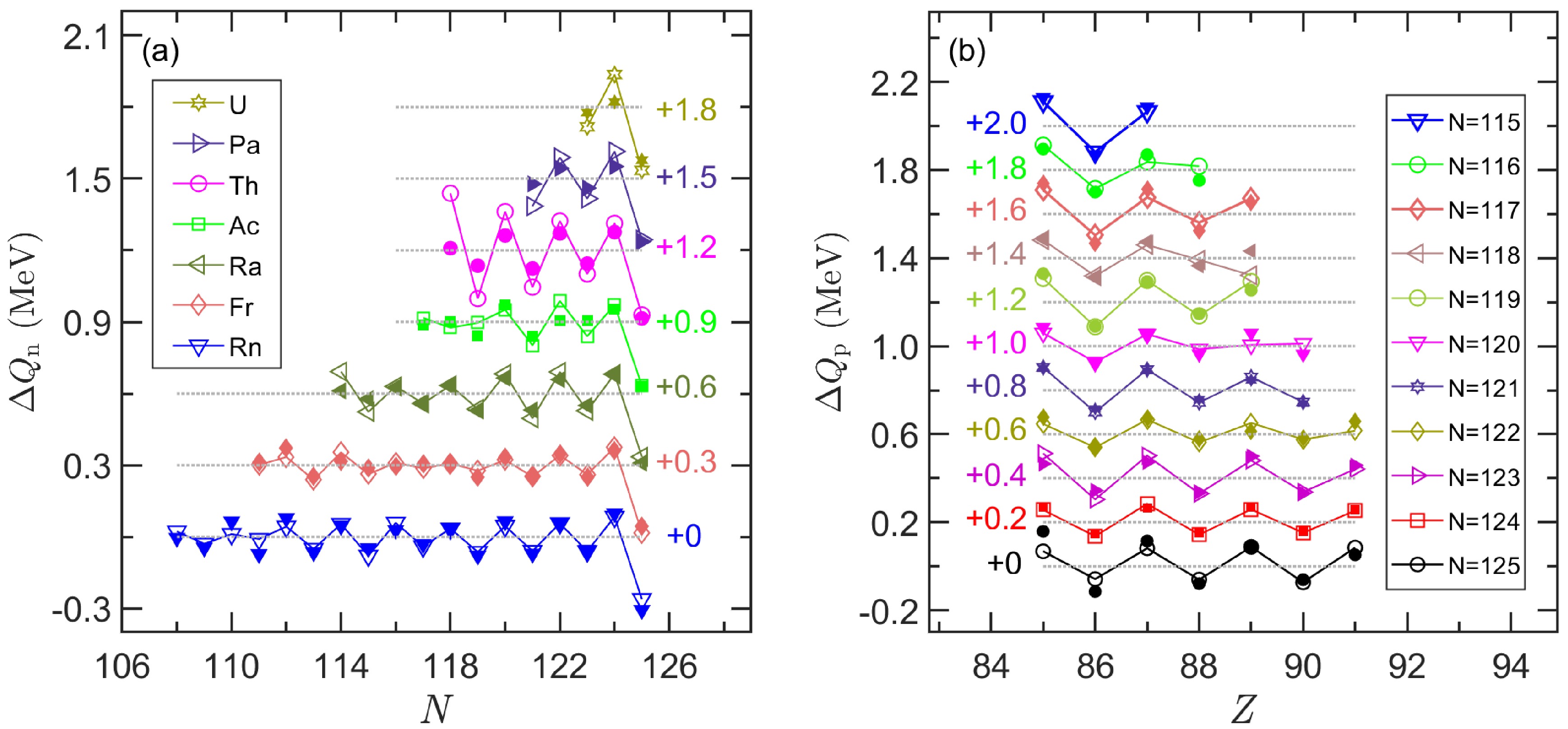

Figure 7.  (Color online) The odd-even staggering (OES) pattern of α-decay energies: (a) neutron OES ($ \Delta Q_{\text{n}} $ in MeV) versus neutron number N and (b) proton OES ($ \Delta Q_{\text{p}} $ in MeV) versus proton number Z. The theoretical values of GKs+FNN and experimental data are represented by hollow and solid symbols, respectively. Most experimental data are obtained from the AME2020 [10, 11], except for $ ^{207,208}\text{Th} $ [76] and $ ^{214,217}\text{U} $[80]. The $ Q_{\alpha} $ energy of $ ^{209}\text{Th} $ has no relevant experimental value, and the solid symbol plotted in the figure is from the theoretical prediction [81]. To avoid overlapping, a small translation is added to the $ \Delta Q_{\text{n}} $/$ \Delta Q_{\text{p}} $ values of each isotopes/isotones (the corresponding value is indicated next to each chain).

To summarize, we employed a feedforward neural network (FNN) to improve three local mass models (GK, GKs, and GK+J). The constructed neural network consists of an input layer, a hidden layer and an output layer. By comparing different combinations of input features, it is found that the physical quantities $ Z_{\text{eo}} $ and $ N_{\text{eo}} $ related to pairing effect can effectively improve the predictive ability of the neural network, thus improving the prediction accuracy of the three local mass models. Our improvements in both description and prediction of mass excess are investigated. For known masses in AME2012, the FNN-improved GK, GKs, and GK+J models achieved better agreement with experimental values, reducing the RMSD to 121 keV, 142 keV, and 165 keV, respectively. However, it is worth noting that the improvement made to the GK model by the FNN is minor on the test set. For the AME2012 to AME2020 extrapolation, the FNN approach reduced the mass RMSD to 311 keV, 328 keV, and 533 keV. In addition, this approach successfully predicted 20 new masses measured experimentally after 2020, reducing the RMSD predicted by the three local mass models to 183 keV, 181 keV and 362 keV, showing strong predictive power. Based on the improved mass data, one- and two-proton/neutron separation energies and α-decay energies are studied, and good optimization results are also obtained. Finally, it should be pointed out that the quantification and representation of model uncertainty are important. Compared with the FNN, the BNN can naturally provide the uncertainties in mass predictions [43]. Therefore, we will consider using the BNN to improve local mass models and evaluate model uncertainty in the future research.

At present, there is little work to improve local mass models based on the neural network, and the work in this paper is a useful attempt. Our results indicate that neural networks provide a new way to further improve the accuracy of local mass model in describing and predicting atomic mass related data in unknown regions. Although this paper achieves high accuracy by applying the FNN to improve three local mass models, there is still a gap between local and global mass models in terms of describing and predicting masses far from known regions. In view of this, an important future direction is to integrate the advantages of local and global models (for instance, incorporating global features into local mass models or embedding local features into global mass models) and apply neural networks for improvement, so as to further enhance the predictive capability for unknown masses.

Thanks to Prof. Meng Wang (Institute of Modern Physics, Chinese Academy of Sciences) for providing the bibliography of new mass measurement after AME2020. Thanks to Man Bao from University of Shanghai for Science and Technology and Chang Ma from Yanshan University for providing the data of GKs and GK+J models respectively.