Production of higher excited quarkonium pair at super Z factory

In comparison with the hardon collider, an electron-positron collider is more suitable for the precise study of the Standard Model (SM) of particle physics because of its much clearer background. An electron-positron collider with high luminosity and running at the $ Z^0 $ boson pole would be a nice platform for such precise study because sizable events of interest can be generated in the $ Z^0 $ decays. For example, the Circular Electron-Positron Collider (CEPC) would have the $ Z^0 $ yields of $ 7\times10^{11} $ per year at the Z-factory mode [1]. We can take precise measurements on the parameters of SM and also probe new physics in the decays of the massive $ Z^0 $ events. The future super Z factory provides not only more yields of the particles we are interested in, but also a supplemental production mechanism in an indirect way.

The heavy quarkonium is a bound state system which consists of a pair of heavy quark and its antiquark. The production of the heavy quarkonium is thought to be a multiscale problem for probing the quantum chromodynamics (QCD) theory. According to the non-relativistic QCD (NRQCD) [2, 3], the heavy quarkonium has three disparate momentum scales: the quark mass $ \sim m_Q $, the momentum of the heavy quark or antiquark $ \sim m_Q v $, and the kinetic energy of the heavy quark or antiquark $ \sim m_Q v^2 $. Here, v is the relative velocity between the heavy quark and antiquark in the quarkonium rest frame. According to the NRQCD factorization framework, the production of the heavy quarkonium can be factored into the short-distance coefficients and the long-distance matrix element. The former depicts the creation of the constituent heavy quark pair $ Q\bar{Q}^\prime $ with definite $ J^{PC} $ quantum numbers that can be calculated perturbatively, while the latter expresses the hadronization of $ Q\bar{Q}^\prime $ pair to a physical color-singlet quarkonium non-perturbatively. Thus the production of the heavy quarkonium has been a hot topic to explore the QCD at both the perturbative and non-perturbative energy regions, which provides rich QCD physics. To obtain more information on the current status of the heavy quarkonium, one may refer to Refs. [4−8].

The production of the heavy quarkonium has been studied widely. Under the NRQCD factorization framework, the next-to-leading order (NLO) corrections in QCD to most of the inclusive and exclusive processes of heavy quarkonium at B factories are calculated. One may refer to Refs. [9−17] for some typical works. For the production of heavy quarkonium at hadron colliders, the NLO calculation for inclusive processes is still challenging. For example, the QCD NLO correction to the $ p+p \longrightarrow J/\psi + c +\bar{c} $ is still missing. Yet we have great advances in the NLO calculation for the exclusive production of double heavy quarkonia, such as double $ J/\psi $ production [18, 19] and the very recent $ B_c $ pair production [20]. Recently, we have the QCD next-to-next-to-leading order (NNLO) corrections to the production of double charmonia at B factories [21, 22]. Very recently, we also have great progress in the automated NLO calculation for heavy quarkonium inclusive and associated production processes [23].

In our previous work, we study the production of double heavy quarkonia at super Z factory [24]. In this work, we continue to study the production of the higher excited double heavy quarkonia, i.e., the heavy quarkonia are in the color-singlet state $ [n^1S_0] $, $ [n^3S_1] $, $ [n^1P_0] $, and $ [n^3P_J](J=0,1,2) $ with $ n=1,2,3 $. The higher excited states would decay into the ground states, and they have significant influence on the production rates of the ground states. We study the production of higher excited heavy quarkonia in the decay of $ W^\pm $, top quark, $ Z^0 $, and Higgs boson [25−29]. The numerical results show that sizable events of those exited $ [nS] $ and $ [nP] $-wave states ($ n \ge 2 $) can be obtained. For example, the contribution of $ 2S $ state would increase the $ 1S $ yield by about 20%$ \sim $50%. It is very necessary to have an estimation of those exited heavy quarkonia though we have begin calculating the NLO and even NNLO corrections. This will give us a complete prediction at leading order (LO).

The rest of the present paper is organized as follows. In Sec. II, we introduce the prescription of the production of higher excited heavy quarkonium pair under the NRQCD framework. In Sec. III, we calculate the total cross sections of $ e^+e^-\to Z^0 \to |(Q\bar{Q^\prime})[n]\rangle + |(Q^\prime \bar{Q})[n']\rangle $ ($ Q,\; Q^\prime=c $- or b-quarks) in color-singlet model, and discuss their differential angle distributions and uncertainties. Sec. IV is reserved for a summary.

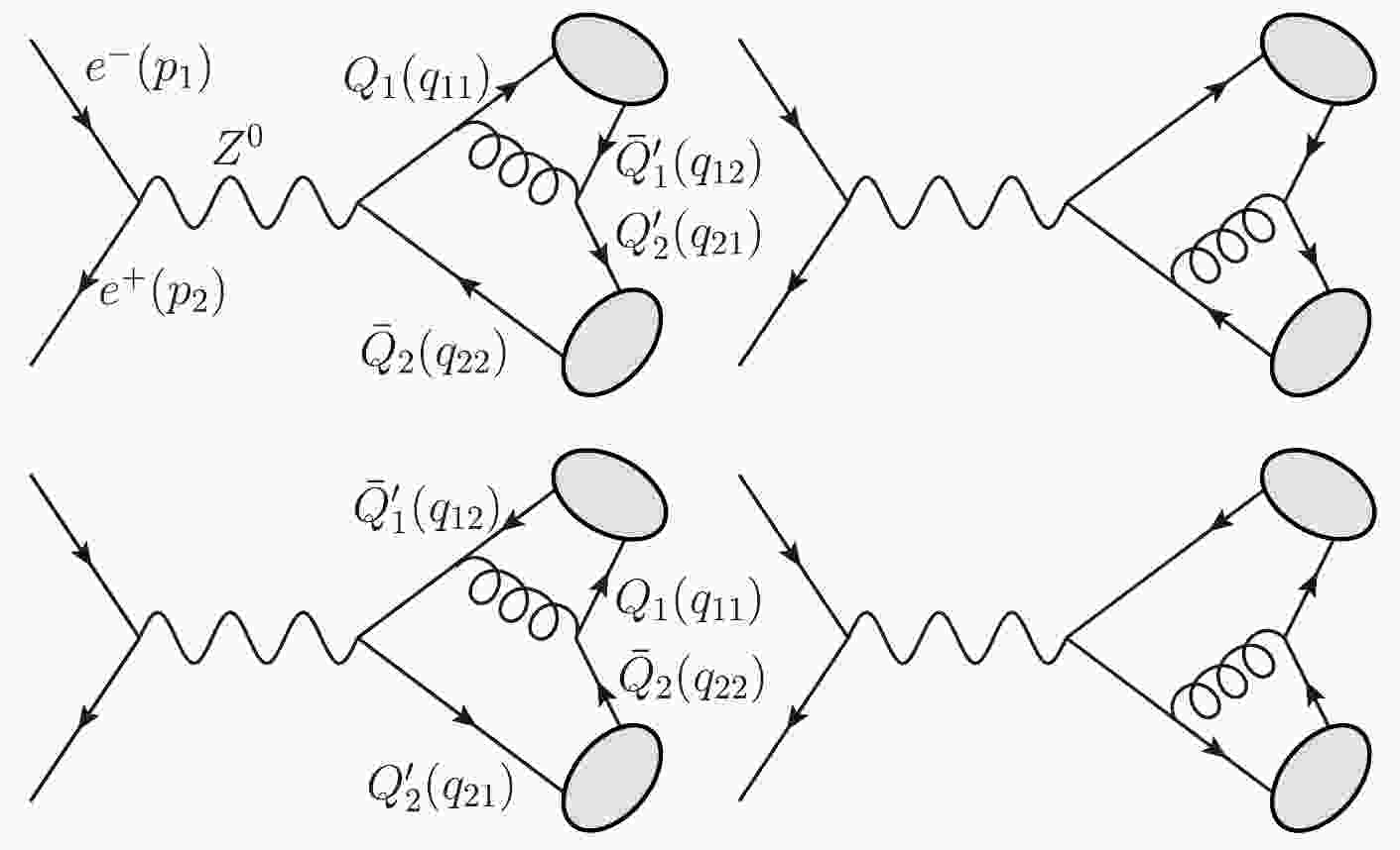
The Feynman diagrams for the production of a pair of higher excited heavy quarkonia via $ e^-(p_1) e^+(p_2) \to Z^0 \to |(Q\bar{Q}^\prime)[n]\rangle (q_1) + |(Q^\prime\bar{Q})[n^\prime]\rangle (q_2) $ are displayed in Fig. 1. According to the QCD factorization formula, its differential cross sections can be factored into the short-distance coefficients and the long-distance matrix elements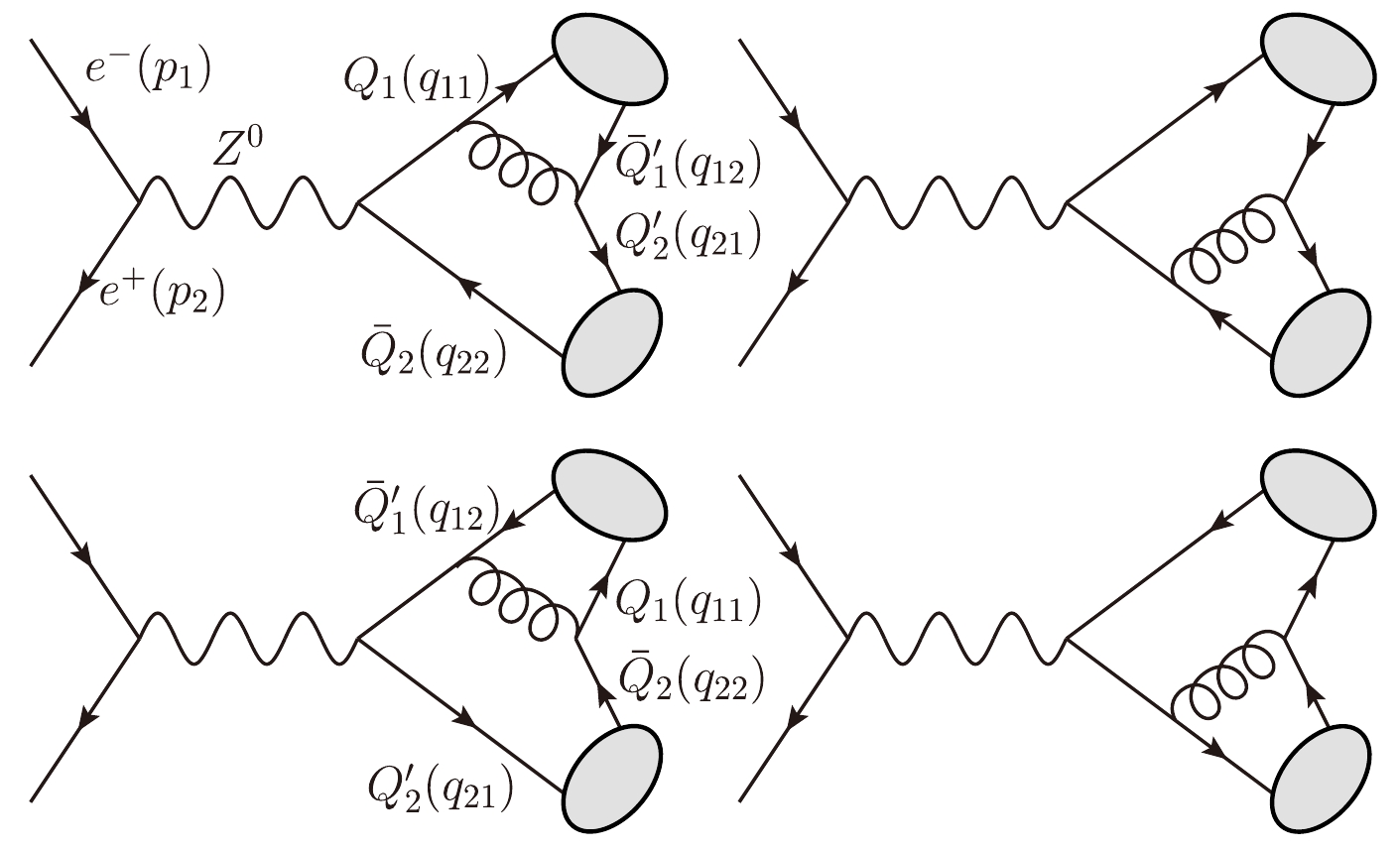

Figure 1.  Feynman diagrams for $ e^-(p_1) e^+(p_2) \to Z^0 \to $$ |(Q\bar{Q}^\prime)[n]\rangle (q_1) + |(Q^\prime\bar{Q})[n^\prime]\rangle (q_2) $, where $ Q,\; Q^\prime=c $-, b-quarks, and $ [n] $ represents the color-singlet $ [n^1S_0], \; [n^3S_1], \; [n^1P_1] $, and $ [n^3P_J] $ ($ n=1,2,3; J=0,1,2 $) heavy quarkonia.

The short-distance coefficients $ \hat\sigma((Q^\prime\bar{Q})[n]+ (Q\bar{Q^\prime})[n^\prime]) $ can be calculated perturbatively, which depicts the short-distance production of two Fock states $ (Q^\prime\bar{Q})[n] $ and $ (Q\bar{Q^\prime})[n^\prime] $ ($ Q^{(\prime)} =b $- or c-quarks) in the spin, color, and angular momentum states $ [n^{(\prime)}] $. Here, the $ [n^{(\prime)}] $ stands for the color-singlet states $ [n^{(\prime)1}S_0], \; [n^{(\prime)3}S_1], \; [n^{(\prime)1}P_1] $, and $ [n^{(\prime)3}P_J] $ ($ n=1,2,3;J=0,1,2 $).

The long-distance matrix elements $ {\langle{\cal O}[n] \rangle} $ is a non-perturbative parameter, which describes the hadronization of the heavy quark pair $ (Q\bar{Q^\prime})[n] $ with quantum number n into the heavy quarkonium $ |(Q\bar{Q^\prime})[n]\rangle $. In the NRQCD framework, we have contributions of both color-singlet state and the color-octect state. In this work, we only consider the color-singlet state, i.e., the intermediate heavy quark pair $ (Q\bar{Q^\prime})[n] $ and the final heavy quarkonium $ |(Q\bar{Q^\prime})[n]\rangle $ have the same quantum number n. The color-singlet matrix elements $ \langle{\cal O}([n]) \rangle $ in Eq. (1) can be related to the Schr$ {\rm \ddot{o}} $dinger wave function at the origin $ \Psi_{\mid(Q\bar{Q^\prime})[nS]\rangle}(0) $ for the $ nS $-wave heavy quarkonia or the first derivative of the wave function at the origin $ \Psi^\prime_{\mid(Q\bar{Q^\prime})[nP]\rangle}(0) $ for the $ nP $-wave heavy quarkonia,

Since the spin-splitting effect at the same n-th level is small, the same values of wave function for both the spin-triplet and spin-singlet Fock states are adopted in our calculation. The Schrödinger wave function at the origin $ \Psi_{|Q\bar{Q^\prime})[nS]\rangle}(0) $ and its first derivative at the origin $ \Psi^{^\prime}_{|(Q\bar{Q^\prime})[nP]\rangle}(0) $ can be further relevant to the radial wave function at the origin $ R_{|(Q\bar{Q^\prime})[nS]\rangle}(0) $ and its first derivative of the radial wave function at the origin $ R^{^\prime}_{|(Q\bar{Q^\prime})[nP]\rangle}(0) $ respectively [2],

The differential cross section $ d\hat\sigma $ can be calculated perturbatively, which can be formulated as

where $ \overline{\sum} $ stands for the average over the spin of the initial positron and electron, and sum over the color and spin of the final higher excited heavy quarkonia. The two-body phase space in the $ e^-e^+ $ center-of-momentum (CM) rest frame can be simplified as

Here, $ s=(p_1+p_2)^2 $ is the squared CM energy. The $ 3 $-momentum of the heavy quarkonium $ |(Q\bar{Q}^\prime) [n]\rangle $ is $ {|\vec{q}_1|}=\sqrt{\lambda[s, M^2_{1}, M^2_{2}] }/2\sqrt{s} $, in which $ \lambda[a, b, c]= (a - b - c)^2 - 4 b c $, and $ M_{1} $ and $ M_{2} $ are the masses of two higher excited heavy quarkonia. θ is the angle between the momentum $ \vec{p_1} $ of the electron and the momentum $ \vec{q_1} $ of the heavy quarkonium $ |(Q\bar{Q}^\prime)[n]\rangle $.

The hard scattering amplitude $ {\cal M}([n],\; [n^\prime]) $ in Eq. (4) can be read directly from the Feynman diagrams in Fig. 1, which can be expressed as

Here k are the number of Feynman diagrams, s and $ s^\prime $ are the spins of the initial electron and positron. The vertex $ \cal{L}^\sigma $ and the propagator $ \cal{D_{\sigma\rho}} $ for $ Z^0 $ propagated processes have the following forms,

In which, $ p=p_1+p_2 $ represents the momentum of the propagator. e denotes the unit of electric charge, $ e_Q=1 $ for the positron and electron, $ e_Q=-1/3 $ for b-quark and $ e_Q=2/3 $ for c-quark. g is the weak interaction coupling constant, $ \theta_W $ stands for the Weinberg angle, and $ \Gamma_Z $ and $ m_Z $ are the total decay width and the mass of $ Z^0 $ boson, respectively.

The concrete expressions of the Dirac γ matrix chains $ {\cal A}^\sigma_k $ in Eq. (6) for the $ nS $-wave spin-singlet $ n^1S_0 $ and spin-triplet $ n^3S_1 $ ($ n=1,2,3 $) can be expressed as

Here, S and L represent the quantum number of spin and orbit angular momentums of the heavy quarkonium, respectively. $ q_{11}=\dfrac{m_{Q_1}}{M_{1}}{q_1} $ and $ q_{12}=\dfrac{m_{Q_1^\prime}}{M_{1}}{q_1} $ are the momenta of the two constituent quarks of the heavy quarkonium $ |(Q\bar{Q}^\prime)[n]\rangle (q_1) $ with $ M_{1}=m_{Q_1}+m_{{Q}_1^\prime} $. $ q_{21}=\dfrac{m_{Q_2^\prime}}{M_{2}}{q_2}+q $ and $ q_{22}=\dfrac{m_{{Q}_2}}{M_{2}}{q_2}-q $ are the momenta of the two heavy constituent quarks of the heavy quarkonium $ |(Q^\prime\bar{Q})[n^\prime]\rangle (q_2) $ with $ M_{2}=m_{Q_2^\prime}+m_{{Q}_2} $. q stands for the relative momentum between the heavy quark $ Q_2^\prime $ and $ {Q}_2 $. We introduce the relative momentum q for the quarkonium $ |(Q^\prime\bar{Q})[n^\prime]\rangle (q_2) $ because it might be either a $ nS $-wave state or a $ nP $-wave state accordingly. For a $ nS $-wave state, the relative momentum q is set to zero directly. In the case of a $ nP $-wave state, we should take derivative of the amplitude over q first and then set $ q=0 $. The two projectors $ \Pi^{(S,L=0)}_{q_k} $ ($ k=1, 2 $) in Eq. (8) have the following forms

Where $ \epsilon_{a}=1 $ and $ \gamma^a=\gamma^5 $ for the spin-singlet $ ^1S_0 $ states ($ S=0,L=0 $), and $ \epsilon_{a}=\varepsilon_{\mu} $ and $ \gamma^a=\gamma^\mu $ for spin-triplet $ ^3S_1 $ state ($ S=1,L=0 $) with μ being the Lorentz vector index. $ \delta_{ij}/\sqrt{N_c} $ denotes the color operator for color-singlet projector with $ N_c=3 $.

In the case of $ |(Q^\prime\bar{Q})[n^\prime]\rangle (q_2) $ being a $ nP $-wave state, the expressions of $ {\cal A}^\sigma_k\; (k=1,2,3,4) $ for the $ nP $-wave spin-singlet states $ n^1P_1\; (S=0,L=1) $ and spin-triplet states $ n^3P_J\; (S=1,L=1) $ with total angular momentum ($ J=0,1,2 $) can be formulated as the first derivative of S-wave amplitudes for the relative momentum q and then set $ q=0 $,

Where $ \varepsilon_\nu(q_2) $ stands for the polarization vector of a $ n^1P_1 $ state, $ \varepsilon^{J}_{\mu\nu}(q_2) $ is the polarization tensor for a $ n^3P_J $ state ($ J=0,1,2 $). The derivative over the relative momentum $ q_{\nu} $ will lead to complicated and lengthy amplitudes. Thus for $ nP $-wave states, it is very time-consuming to get the squared amplitudes $ |{\cal M}([n],[n^\prime])|^{2} $ using the traditional method. We continue using the "improved trace technique" to deal with the amplitudes $ {\cal M}([n],[n^\prime]) $. In ths prescription, the compact analytical expressions of the complicated $ nP $-wave can be obtained, and the efficiency of numerical evaluation can also be improved. To shorten the present paper, we don't further introduce the "improved trace technique" in details. For complete techniques and typical examples, please refer to literatures [25, 29−33].

When handling the squared amplitudes $ |{\cal M}([n],[n^\prime])|^{2} $, we also need to sum over the polarization vectors or tensors of the heavy quarkonia. The polarization sum for the spin-triplet $ n^3S_1 $ states or the spin-singlet $ n^1P_1 $ states with momentum p is given by [3]

where $ J_z=S_z $ and $ L_z $ stand for $ n^3S_1 $ and $ n^1P_1 $ states, respectively. The sum over the polarization tensors of $ n^3P_J $ states can be obtained by [3]

For numerical evaluations, the masses of the constituent charm and bottom quarks for the heavy quarkonia $ |(Q\bar{Q^\prime})[n]\rangle $ and $ |(Q^\prime\bar{Q})[n^\prime]\rangle $ are displayed in Table 1. The mass of the higher excited heavy quarkonium is set to be the sum of the masses of its constituent quarks at the same order n-th. This is assured by the gauge invariance of amplitudes within the NRQCD framework. The radial wave functions at the origin $ R_{|(Q\bar{Q^\prime})[nS]\rangle}(0) $ and their first derivatives at the origin $ R^\prime_{|(Q\bar{Q}^\prime)[nP]\rangle}(0) $ for heavy quarkonium $ |(Q\bar{Q^\prime})[n]\rangle $ have been calculated under five different potential models in our previous work [26]. Because the Buchmüller and Tye potential model (BT-potential) [34, 35] has the correct two-loop short-distance behavior in the QCD, we adopt the results of the BT-potential in the present work, which has been displayed in Table 1. The uncertainties of $ R_{|(Q\bar{Q})[nS]\rangle}(0) $ and $ R'_{|(Q\bar{Q})[nP]\rangle}(0) $ are induced by the corresponding varying constituent quark masses. They will be taken into consideration when we discuss the uncertainties of the total cross sections caused by the varying quark masses in Sec. 3.3. The leading-order running strong coupling constant $ \alpha_s=0.26 $ is adopted for $ |(c\bar{c})[n]\rangle $ and $ |(b\bar{c})[n]\rangle $, and $ \alpha_s=0.18 $ for $ |(b\bar{b})[n]\rangle $. Other parameters are derived from the PDG [36].

	$ m_c $, $ |R_{|(c\bar{c})[nS]\rangle}(0)|^2 $	$ m_c $, $ |R'_{|(c\bar{c})[nP]\rangle}(0)|^2 $
$ n=1 $	1.48$ \pm $0.1, $ 2.458^{+0.227}_{-0.327} $	1.75$ \pm $0.1, $ 0.322^{+0.077}_{-0.068} $
$ n=2 $	1.82$ \pm $0.1, $ 1.671^{+0.115}_{-0.107} $	1.96$ \pm $0.1, $ 0.224^{+0.012}_{-0.012} $
$ n=3 $	1.92$ \pm $0.1, $ 0.969^{+0.063}_{-0.057} $	2.12$ \pm $0.1, $ 0.387^{+0.045}_{-0.042} $
	$ m_b $, $ |R_{|(b\bar{b})[nS]\rangle}(0)|^2 $	$ m_b $, $ |R'_{|(b\bar{b})[nP]\rangle}(0)|^2 $
$ n=1 $	4.71$ \pm $0.2, $ 16.12^{+1.28}_{-1.23} $	4.94$ \pm $0.2, $ 5.874^{+0.728}_{-0.675} $
$ n=2 $	5.01$ \pm $0.2, $ 6.746^{+0.598}_{-0.580} $	5.12$ \pm $0.2, $ 2.827^{+0.492}_{-0.432} $
$ n=3 $	5.17$ \pm $0.2, $ 2.172^{+0.178}_{-0.155} $	5.20$ \pm $0.2, $ 2.578^{+0.187}_{-0.186} $
	$ m_c $ /$ m_b $, $ |R_{|(c\bar{b})[nS]\rangle}(0)|^2 $	$ m_c $ /$ m_b $, $ |R'_{|(c\bar{b})[nP]\rangle}(0)|^2 $
$ n=1 $	1.45$ \pm $0.1 /4.85$ \pm $0.2, $ 3.848^{+0.238}_{-0.225} $	1.75$ \pm $0.1 /4.93$ \pm $0.2, $ 0.518^{+0.122}_{-0.105} $
$ n=2 $	1.82$ \pm $0.1 /5.03$ \pm $0.2, $ 1.987^{+0.116}_{-0.118} $	1.96$ \pm $0.1 /5.13$ \pm $0.2, $ 0.500^{+0.036}_{-0.036} $
$ n=3 $	1.96$ \pm $0.1 /5.15$ \pm $0.2, $ 1.347^{+0.079}_{-0.082} $	2.15$ \pm $0.1 /5.25$ \pm $0.2, $ 0.729^{+0.080}_{-0.075} $

Table 1.  Masses (units: GeV) of the constituent heavy quarks, the radial wave functions at the origin $ |R_{|(Q\bar{Q}^\prime)[nS]\rangle}(0)|^2 $ (units: GeV$ ^3 $) and their first derivatives at the origin $ |R'_{|(Q\bar{Q}^\prime)[nP]\rangle}(0)|^2 $ (units: GeV$ ^5 $) under the BT-potential [26]. Note, the uncertainties of $ R_{|(Q\bar{Q})[nS]\rangle}(0) $ and $ R'_{|(Q\bar{Q})[nP]\rangle}(0) $ are induced by the corresponding varying constituent quark masses.

The total cross sections for the production of the higher excited heavy quarkonium pair in $ e^-e^+\to Z^0\to |(Q\bar{Q^\prime})[n]\rangle+|(Q^\prime\bar{Q})[n']\rangle $ ($ Q,\; Q^\prime=c $- or b-quarks) at CM energy $ \sqrt{s}=91.1876 $ GeV are listed in Tabs. 2-4 for double charmonium, double bottomonium, and $ B_c $ pair, respectively. Where the uncertainties are caused by the varying quark masses. The charm quark mass $ m_c $ has the variation $ \pm 0.1 $ GeV, and the bottom quark mass $ m_b $ has the variation $ \pm 0.2 $ GeV. In Tabs. 2-4, the top three rankings are marked in bold. For the double charmonium channels, we always have $ \sigma_{(|(c\bar{c})[n^3S_1]\rangle+|(c\bar{c})[n'^1P_1]\rangle)} > \sigma_{(|(c\bar{c})[n^1S_0]\rangle+|(c\bar{c})[n'^3P_2]\rangle)} > \sigma_{(|(c\bar{c})[n^1S_0]\rangle+|(c\bar{c})[n'^3P_0]\rangle)} $ at the same nth level. For double bottomonium channels, the largest cross sections can either be the $ |(b\bar{b})[n^1S_0]\rangle+|(b\bar{b})[n'^3S_1]\rangle $ or $ |(b\bar{b})[n^3S_1]\rangle+|(b\bar{b})[n'^3P_2]\rangle $. For $ B_c $ pair channel, the largest cross section can either be $ |(c\bar{b})[n^3S_1]\rangle+|(b\bar{c})[n'^3S_1]\rangle $ or $ |(c\bar{b})[n^3S_1]\rangle+|(b\bar{c})[n'^3P_2]\rangle $. Note, in Tabs. 2-4 we have redundant data in the row of $ \sigma_{(|(Q\bar{Q}^\prime)[n^3S_1]\rangle+|(Q\bar{Q}^\prime)[n'^3S_1]\rangle)} $, i.e., the cross sections are the same when n and $ n^\prime $ being exchanged. This is also a check for our massive calculations.

$ [n]+[n^\prime] $	1+1	1+2	1+3	2+1	2+2	2+3	3+1	3+2	3+3
$ \sigma_{([n^1S_0]+[n'^3S_1])} $	$ 18.95^{+3.64}_{-4.70} $	$ 11.32^{+1.98}_{-2.20} $	$ 6.632^{+1.121}_{-1.250} $	$ 13.91^{+2.24}_{-2.55 } $	$ 8.176^{+1.19}_{-1.04} $	$ 4.770^{+0.672}_{-0.579} $	$ 8.594^{+1.308}_{-1.506} $	$ 5.032^{+0.694}_{-0.598} $	$ 2.933^{+0.390}_{-0.332} $
$ \sigma_{([n^3S_1]+[n'^3S_1])} $	$ 64.16^{+12.29}_{-15.87} $	$ 42.55^{+7.09}_{-8.00} $	$ 25.63^{+4.08}_{-4.64} $	$ 42.55^{+7.09}_{-8.00} $	$ 27.62^{+4.01}_{-3.49} $	$ 16.55^{+2.29}_{-1.98} $	$ 25.63^{+4.08}_{-4.64} $	$ 16.55^{+2.29}_{-1.98} $	$ 9.900^{+1.308}_{-1.099} $
$ \sigma_{([n^1S_0]+[n'^1P_1])} $	$ 60.76^{+4.49}_{-7.35} $	$ 18.71^{+1.35}_{-0.57} $	$ 25.47^{+0.16}_{-1.04} $	$ 20.42^{+1.32}_{-1.43} $	$ 10.07^{+1.04}_{-0.80} $	$ 13.69^{+0.26}_{-0.19} $	$ 11.63^{+0.72}_{-0.76} $	$ 5.729^{+0.572}_{-0.468} $	$ 7.792^{+0.184}_{-0.128} $
$ \sigma_{([n^3S_1]+[n'^1P_1])} $	$ {454.0}^{+39.1}_{-59.2} $	$ {227.1}^{+4.4}_{-14.0} $	$ {312.4}^{+1.8}_{-16.2} $	$ {247.4}^{+19.0}_{-19.7} $	$ {123.8}^{+10.2}_{-8.4} $	$ {170.6}^{+0.6}_{-0.2} $	$ {141.3}^{+10.4}_{-10.7} $	$ {70.77}^{+6.18}_{-5.00} $	$ {97.48}^{+1.11}_{-0.41} $
$ \sigma_{([n^1S_0]+[n'^3P_0])} $	$ {137.0}^{+9.9}_{-16.4} $	$ {68.03}^{+2.17}_{-5.01} $	$ {93.16}^{+0.70}_{-3.71} $	$ {72.27}^{+4.44}_{-4.85} $	$ {35.87}^{+3.50}_{-2.93} $	$ {49.10}^{+1.04}_{-0.79} $	$ {40.87}^{+2.47}_{-2.65} $	$ {20.29}^{+2.09}_{-1.71} $	$ {27.76}^{+0.73}_{-0.53} $
$ \sigma_{([n^1S_0]+[n'^3P_1])} $	$ 18.87^{+3.98}_{-4.27} $	$ 10.56^{+0.41}_{-0.90} $	$ 15.74^{+1.69}_{-2.28} $	$ 12.37^{+2.30}_{-2.10} $	$ 6.835^{+0.136}_{-0.117} $	$ 10.11^{+0.89}_{-0.82} $	$ 7.432^{+1.327}_{-1.213} $	$ 4.093^{+0.058}_{-0.038} $	$ 6.039^{+0.496}_{-0.448} $
$ \sigma_{([n^1S_0]+[n'^3P_2])} $	$ {284.2}^{+22.2}_{-35.3} $	$ {140.9}^{+3.8}_{-9.7} $	$ {192.4}^{+0.5}_{-8.5} $	$ {153.2}^{+10.5}_{-11.2} $	$ {75.96}^{+5.51}_{-6.91} $	$ {103.8}^{+1.0}_{-1.6} $	$ {87.22}^{+5.69}_{-5.97} $	$ {43.26}^{+3.39}_{-4.16} $	$ {59.13}^{+0.75}_{-1.18} $
$ \sigma_{([n^3S_1]+[n'^3P_0])} $	$ 44.03^{+4.60}_{-6.38} $	$ 21.89^{+0.95}_{-0.01} $	$ 30.20^{+0.80}_{-2.2} $	$ 25.92^{+2.31}_{-2.33} $	$ 12.76^{+0.85}_{-0.69} $	$ 17.50^{+0.27}_{-0.17} $	$ 15.15^{+1.28}_{-1.27} $	$ 7.437^{+0.542}_{-0.431} $	$ 10.18^{+0.12}_{-0.04} $
$ \sigma_{([n^3S_1]+[n'^3P_1])} $	$ 17.62^{+3.57}_{-3.88} $	$ 10.79^{+0.29}_{-0.80} $	$ 17.07^{+1.59}_{-2.26} $	$ 9.625^{+1.822}_{-1.663} $	$ 5.909^{+0.105}_{-0.086} $	$ 9.354^{+0.774}_{-0.711} $	$ 5.492^{+1.019}_{-0.926} $	$ 3.374^{+0.048}_{-0.032} $	$ 5.344^{+0.423}_{-0.380} $
$ \sigma_{([n^3S_1]+[n'^3P_2])} $	$ 57.51^{+8.25}_{-10.02} $	$ 24.83^{+0.06}_{-1.18} $	$ 38.15^{+2.66}_{-4.20} $	$ 22.09^{+3.70}_{-3.42} $	$ 13.26^{+0.08}_{-0.01} $	$ 20.55^{+1.33}_{-1.19} $	$ 12.46^{+2.08}_{-1.92} $	$ 7.521^{+0.015}_{-0.069} $	$ 11.69^{+0.73}_{-0.64} $

Table 2.  The total cross sections (units: $ \times 10^{-5}\; fb $) for the production of higher excited charmonium pair in $ e^+e^-\to Z^0 \to $$ |(c\bar{c})[n]\rangle +|(c\bar{c})[n^\prime]\rangle $ at $ \sqrt{s}=91.1876 $ GeV. The uncertainties are caused by the varying charm quark mass by 0.1 GeV, where effects of the uncertainties of the $ R_{|(c\bar{c})[nS]\rangle}(0) $ and $ R'_{|(c\bar{c})[nP]\rangle}(0) $ induced by varying masses are also considered (see Table 1 for explicit values). The top three rankings are marked in bold.

$ [n]+[n^\prime] $	1+1	1+2	1+3	2+1	2+2	2+3	3+1	3+2	3+3
$ \sigma_{([n^1S_0]+|[n'^3S_1])} $	$ {428.6}^{+67.9}_{-60.9} $	$ {173.3}^{+29.4}_{-26.9} $	$ {54.82}^{+8.92}_{-7.61} $	$ {184.3}^{+30.7}_{-27.6} $	$ {74.40}^{+13.23}_{-11.87} $	$ {23.53}^{+4.03}_{-3.45} $	$ {60.18}^{+9.54}_{-8.15} $	$ {24.28}^{+4.12}_{-3.53} $	$ {7.675}^{+1.25}_{-1.02} $
$ \sigma_{([n^3S_1]+[n'^3S_1])} $	$ {119.9}^{+18.4}_{-16.6} $	$ 49.84^{+8.14}_{-7.08} $	$ 16.00^{+2.47}_{-2.16} $	$ {49.84}^{+8.14}_{-7.08} $	$ 20.69^{+3.58}_{-3.23} $	$ 6.634^{+1.097}_{-0.946} $	$ 16.00^{+2.47}_{-2.16} $	$ 6.634^{+1.097}_{-0.946} $	$ 2.127^{+0.336}_{-0.274} $
$ \sigma_{([n^1S_0]+[n'^1P_1])} $	$ 53.27^{+1.46}_{-1.51} $	$ 22.83^{+1.77}_{-1.68} $	$ 19.80^{+0.25}_{-0.28} $	$ 21.08^{+0.82}_{-0.68} $	$ 9.036^{+0.809}_{-0.778} $	$ 7.835^{+0.024}_{-0.007} $	$ 6.601^{+0.225}_{-0.119} $	$ 2.829^{+0.238}_{-0.206} $	$ 2.453^{+0.033}_{-0.019} $
$ \sigma_{([n^3S_1]+[n'^1P_1])} $	$ 61.46^{+4.22}_{-4.05} $	$ 26.91^{+3.25}_{-2.95} $	$ 23.55^{+0.60}_{-0.63} $	$ 24.90^{+1.99}_{-1.72} $	$ 10.90^{+1.44}_{-1.32} $	$ 9.543^{+0.347}_{-0.374} $	$ 7.891^{+0.586}_{-0.434} $	$ 3.454^{+0.437}_{-0.373} $	$ 3.024^{+0.093}_{-0.075} $
$ \sigma_{([n^1S_0]+|([n'^3P_0])} $	$ 9.215^{+0.141}_{-0.160} $	$ 4.010^{+0.262}_{-0.256} $	$ 3.501^{+0.081}_{-0.088} $	$ 3.495^{+0.087}_{-0.067} $	$ 1.520^{+0.114}_{-0.113} $	$ 1.327^{+0.015}_{-0.021} $	$ 1.068^{+0.020}_{-0.004} $	$ 0.465^{+0.032}_{-0.028} $	$ 0.405^{+0.011}_{-0.009} $
$ \sigma_{([n^1S_0]+[n'^3P_1])} $	$ 14.31^{+1.60}_{-1.60} $	$ 6.331^{+1.041}_{-0.925} $	$ 5.568^{+0.362}_{-0.368} $	$ 6.049^{+0.725}_{-0.635} $	$ 2.672^{+0.463}_{-0.412} $	$ 2.349^{+0.172}_{-0.176} $	$ 1.959^{+0.220}_{-0.176} $	$ 0.865^{+0.143}_{-0.121} $	$ 0.760^{+0.050}_{-0.045} $
$ \sigma_{([n^1S_0]+|[n'^3P_2])} $	$ 28.15^{+1.38}_{-1.35} $	$ 12.15^{+1.22}_{-1.13} $	$ 10.57^{+0.071}_{-0.087} $	$ 11.36^{+0.69}_{-0.59} $	$ 4.903^{+0.55}_{-0.51} $	$ 4.265^{+0.077}_{-0.091} $	$ 3.591^{+0.199}_{-0.136} $	$ 1.550^{+0.166}_{-0.142} $	$ 1.349^{+0.017}_{-0.010} $
$ \sigma_{([n^3S_1]+[n'^3P_0])} $	$ 68.37^{+6.17}_{-5.83} $	$ 30.69^{+4.38}_{-3.92} $	$ 27.16^{+1.24}_{-1.26} $	$ 27.39^{+2.78}_{-2.41} $	$ 12.29^{+1.90}_{-1.70} $	$ 10.88^{+0.61}_{-0.63} $	$ 8.629^{+0.824}_{-0.639} $	$ 3.871^{+0.574}_{-0.486} $	$ 3.425^{+0.173}_{-0.150} $
$ \sigma_{([n^3S_1]+[n'^3P_1])} $	$ 117.5^{+13.6}_{-15.0} $	$ {54.03}^{+9.03}_{-7.98} $	$ {48.32}^{+3.24}_{-3.25} $	$ 46.76^{+5.93}_{-5.16} $	$ {21.50}^{+3.85}_{-3.40} $	$ {19.23}^{+1.50}_{-1.51} $	$ {14.68}^{+1.75}_{-1.44} $	$ {6.748}^{+1.166}_{-0.981} $	$ {6.034}^{+0.436}_{-0.391} $
$ \sigma_{([n^3S_1]+[n'^3P_2])} $	$ {230.6}^{+23.6}_{-22.2} $	$ {104.8}^{+16.2}_{-14.4} $	$ {93.29}^{+5.3}_{-10.5} $	$ {91.99}^{+10.5}_{-9.08} $	$ {41.81}^{+6.97}_{-6.19} $	$ {37.20}^{+2.49}_{-2.53} $	$ {28.90}^{+3.12}_{-46} $	$ {13.13}^{+2.11}_{-1.78} $	$ {11.69}^{+0.72}_{-0.63} $

Table 3.  The total cross sections (units: $ \times 10^{-4} fb $) for the production of higher excited bottomonium pair in $ e^+e^-\to Z^0 \to $$ |(b\bar{b})[n]\rangle +|(b\bar{b})[n^\prime]\rangle $ at $ \sqrt{s}=91.1876 $ GeV. The uncertainties are caused by the varying bottom quark mass by 0.2 GeV, where effects of the uncertainties of the $ R_{|(b\bar{b})[nS]\rangle}(0) $ and $ R'_{|(b\bar{b})[nP]\rangle}(0) $ induced by varying masses are also considered (see Table 1 for explicit values). The top three rankings are marked in bold.

$ [n]+[n^\prime] $	1+1	1+2	1+3	2+1	2+2	2+3	3+1	3+2	3+3
$ \sigma_{([n^1S_0]+[n'^3S_1])} $	$ {634.6}^{+47.8}_{-45.8} $	$ 212.9^{+5.7}_{-3.9} $	$ 127.9^{+2.3}_{-1.6} $	$ {220.3}^{+5.9}_{-41} $	$ 72.63^{+0.30}_{-0.29} $	$ 43.41^{+0.47}_{-0.57} $	$ {133.9}^{+2.4}_{-1.7} $	$ 43.89^{+0.47}_{-0.67} $	$ 26.19^{+1.34}_{-0.58} $
$ \sigma_{([n^3S_1]+[n'^3S_1])} $	$ {1150}^{+87}_{-84} $	$ {397.2}^{+10.5}_{-7.4} $	$ {240.5}^{+4.3}_{-3.1} $	$ {397.2}^{+10.5}_{-7.4} $	$ {136.3}^{+0.6}_{-0.1} $	$ {82.33}^{+0.72}_{-0.94} $	$ {240.5}^{+4.3}_{-3.1} $	$ {82.33}^{+0.72}_{-0.94} $	$ {49.69}^{+0.75}_{-1.00} $
$ \sigma_{([n^1S_0]+[n'^1P_1])} $	$ 4.810^{+0.399}_{-0.406} $	$ 2.134^{+0.154}_{-0.141} $	$ 1.405^{+0.033}_{-0.045} $	$ 2.747^{+0.021}_{-0.024} $	$ 1.357^{+0.148}_{-0.129} $	$ 1.042^{+0.035}_{-0.034} $	$ 1.840^{+0.016}_{-0.022} $	$ 0.926^{+0.100}_{-0.089} $	$ 0.729^{+0.027}_{-0.026} $
$ \sigma_{([n^3S_1]+[n'^1P_1])} $	$ 11.77^{+1.10}_{-1.12} $	$ 8.984^{+0.985}_{-0.784} $	$ 6.849^{+0.344}_{-0.256} $	$ 2.878^{+0.182}_{-0.174} $	$ 2.122^{+0.128}_{-0.114} $	$ 2.510^{+0.013}_{-0.009} $	$ 1.586^{+0.108}_{0.105-} $	$ 1.153^{+0.057}_{-0.053} $	$ 1.355^{+0.008}_{-0.010} $
$ \sigma_{([n^1S_0]+[n'^3P_0])} $	$ 15.27^{+1.10}_{-1.12} $	$ 12.01^{+1.67}_{-1.35} $	$ 14.96^{+1.37}_{-1.12} $	$ 4.430^{+0.205}_{-0.226} $	$ 3.500^{+0.328}_{-0.300} $	$ 4.378^{+0.217}_{-0.204} $	$ 2.536^{+0.140}_{-0.157} $	$ 2.006^{+0.163}_{-0.155} $	$ 2.512^{+0.095}_{-0.097} $
$ \sigma_{([n^1S_0]+[n'^3P_1])} $	$ 6.162^{+0.701}_{-0.448} $	$ 4.751^{+0.443}_{-0.352} $	$ 5.659^{+0.242}_{-0.174} $	$ 1.451^{+0.151}_{-0.145} $	$ 1.161^{+0.041}_{-0.038} $	$ 1.419^{+0.014}_{-0.0137} $	$ 0.780^{+0.093}_{-0.090} $	$ 0.632^{+0.008}_{-0.013} $	$ 0.781^{+0.017}_{-0.019} $
$ \sigma_{([n^1S_0]+[n'^3P_2])} $	$ 3.093^{+0.253}_{-0.236} $	$ 1.326^{+0.214}_{-0.163} $	$ 1.802^{+0208}_{-0.159} $	$ 0.541^{+0.050}_{-0.049} $	$ 0.472^{+0.025}_{-0.023} $	$ 0.628^{+0.009}_{-0.007} $	$ 0.266^{+0.030}_{-0.0296} $	$ 0.236^{+0.007}_{-0.007} $	$ 0.319^{+0.001}_{-0.002} $
$ \sigma_{([n^3S_1]+[n'^3P_0])} $	$ 454.2^{+15.7}_{-30.8} $	$ {239.3}^{+56.8}_{-42.4} $	$ {213.1}^{+33.5}_{-26.1} $	$ 153.3^{+12.5}_{-10.78} $	$ {79.95}^{+16.38}_{-12.9}0 $	$ {70.46}^{+8.89}_{-7.40} $	$ 91.71^{+6.72}_{-5.99} $	$ {47.74}^{+9.32}_{-7.48} $	$ {41.98}^{+4.91}_{-4.20} $
$ \sigma_{([n^3S_1]+[n'^3P_1])} $	$ 270.1^{+16.2}_{-15.8} $	$ 180.1^{+25.2}_{-20.0} $	$ 194.7^{+15.7}_{-12.5} $	$ 84.10^{+2.73}_{-2.56} $	$ 55.80^{+5.52}_{-4.81} $	$ 60.11^{+2.53}_{-2.27} $	$ 49.46^{+1.83}_{-1.98} $	$ 32.77^{+2.88}_{-2.60} $	$ 35.27^{+1.11}_{-1.08} $
$ \sigma_{([n^3S_1]+[n'^3P_2])} $	$ {1133}^{+16}_{-22} $	$ {394.1}^{+89.4}_{-67.1} $	$ {595.3}^{+80.1}_{-62.6} $	$ {376.9}^{+22.5}_{-19.1} $	$ {207.9}^{+37.3}_{-29.8} $	$ {193.6}^{+19.9}_{-16.7} $	$ {224.8}^{+11.5}_{-10.2} $	$ {123.7}^{+21.0}_{-17.1} $	$ {114.9}^{+20.7}_{-9.3} $

Table 4.  The total cross sections (units: $ \times 10^{-3}\; fb $) for the production of higher excited $ B_c $ pair in $ e^+e^-\to Z^0 \to |(c\bar{b})[n]\rangle +|(b\bar{c})[n^\prime]\rangle $ at $ \sqrt{s}=91.1876 $ GeV. The uncertainties are caused by the varying charm quark mass by 0.1 GeV and bottom quark mass by 0.2 GeV, where effects of the uncertainties of the $ R_{|(c\bar{b})[nS]\rangle}(0) $ and $ R'_{|(c\bar{b})[nP]\rangle}(0) $ caused by varying masses are also considered (see Table 1 for explicit values). The top three rankings are marked in bold

As shown in Tabs. 2-4, in comparison with the $ "1+1" $ configuration, the cross sections for the production of higher excited heavy quarkonium pair are sizable. Since most of the higher excited heavy quarkonia will decay to ground states with $ n=1 $, their contribution has to be taken into consideration carfully when we study the production rates of the ground states.

● For the top three double charmonium channels $ |(c\bar{c})[n^3S_1]\rangle+|(c\bar{c})[n'^1P_1]\rangle $, $ |(c\bar{c})[n^1S_0]\rangle+|(c\bar{c})[n'^3P_2]\rangle $, and $ |(c\bar{c})[n^1S_0]\rangle+|(c\bar{c})[n'^3P_0]\rangle $, the total cross sections of $ [1]+[2] $, $ [1]+[3] $, $ [2]+[1] $, $ [2]+[2] $, $ [2]+[3] $, $ [3]+[1] $, $ [3]+[2] $, and $ [3]+[3] $ configurations are about 50%, 69%, 54%, 27%, 38%, 31%, 16%, and 21% of the cross section of the $ [1]+[1] $ configuration, respectively. It is very interesting that the top three double charmonium channels have very similar ratios for other configurations to the $ [1]+[1] $ configuration.

● For the double bottomonium channel $ |(b\bar{b})[n^1S_0]\rangle+ |(b\bar{b})[n'^3S_1]\rangle $, the total cross sections of $ [1]+[2] $, $ [1]+[3] $, $ [2]+[1] $, $ [2]+[2] $, $ [2]+[3] $, $ [3]+[1] $, $ [3]+[2] $, and $ [3]+[3] $ configurations are about 40%, 13%, 43%, 17%, 5.5%, 14%, 5.7%, and 1.8% of the cross section of $ [1]+[1] $ configuration, respectively.

For the double bottomonium channel $ |(b\bar{b})[n^3S_1]\rangle+ |(b\bar{b})[n'^3P_1]\rangle $, the total cross sections of $ [1]+[2] $, $ [1]+[3] $, $ [2]+[1] $, $ [2]+[2] $, $ [2]+[3] $, $ [3]+[1] $, $ [3]+[2] $, and $ [3]+[3] $ configurations are about 46%, 41%, 40%, 18%, 16%, 12%, 5.7%, and 5.1% of the cross section of $ [1]+[1] $ configuration, respectively.

For the double bottomonium channel $ |(b\bar{b})[n^3S_1]\rangle+ |(b\bar{b})[n'^3P_2]\rangle $, the total cross sections of $ [1]+[2] $, $ [1]+[3] $, $ [2]+[1] $, $ [2]+[2] $, $ [2]+[3] $, $ [3]+[1] $, $ [3]+[2] $, and $ [3]+[3] $ configurations are about 45%, 40%, 40%, 18%, 16%, 13%, 5.7%, and 5.1% of the cross section of $ [1]+[1] $ configuration, respectively.

● For the $ B_c $ pair channel $ |(c\bar{b})[n^1S_0]\rangle+|(b\bar{c})[n'^3S_1]\rangle $, the total cross sections of $ [1]+[2] $, $ [1]+[3] $, $ [2]+[1] $, $ [2]+[2] $, $ [2]+[3] $, $ [3]+[1] $, $ [3]+[2] $, and $ [3]+[3] $ configurations are about 34%, 20%, 35%, 11%, 6.8%, 21%, 6.9%, and 4.1% of the cross section of $ [1]+[1] $ configuration, respectively.

For the $ B_c $ pair channel $ |(c\bar{b})[n^3S_1]\rangle+|(b\bar{c})[n'^3S_1]\rangle $, the total cross sections of $ [1]+[2] $, $ [1]+[3] $, $ [2]+[1] $, $ [2]+[2] $, $ [2]+[3] $, $ [3]+[1] $, $ [3]+[2] $, and $ [3]+[3] $ configurations are about 35%, 21%, 35%, 18%, 7.2%, 21%, 7.2%, and 4.3% of the cross section of $ [1]+[1] $ configuration, respectively.

For the $ B_c $ pair channel $ |(c\bar{b})[n^3S_1]\rangle+|(b\bar{c})[n'^3P_2]\rangle $, the total cross sections of $ [1]+[2] $, $ [1]+[3] $, $ [2]+[1] $, $ [2]+[2] $, $ [2]+[3] $, $ [3]+[1] $, $ [3]+[2] $, and $ [3]+[3] $ configurations are about 35%, 53%, 33%, 18%, 17%, 20%, 11%, and 10% of the cross section of $ [1]+[1] $ configuration, respectively.

When CEPC running in the Z factory operation mode, its designed integrated luminosity with two interaction points can reach as high as $ 16\; ab^{-1} $ [1]. Then we can estimate the events of the production of double higher excited heavy quarkonia. We show the events in Table 5 for the top three channels in Tabs. 2-4 as an illustration.

$ [n]+[n^\prime] $	1+1	1+2	1+3	2+1	2+2	2+3	3+1	3+2	3+3
$ |(c\bar{c})[n^3S_1]\rangle+|(c\bar{c})[n'^1P_1]\rangle $	73	37	50	40	20	27	23	11	16
$ |(c\bar{c})[n^1S_0]\rangle+|(c\bar{c})[n'^3P_2]\rangle $	45	22	30	24	12	16	14	7	9
$ |(c\bar{c})[n^1S_0]\rangle+|(c\bar{c})[n'^3P_0]\rangle $	22	11	15	12	6	8	7	3	4
$ |(b\bar{b})[n^1S_0]\rangle+|(b\bar{b})[n'^3S_1]\rangle $	686	277	88	295	119	38	96	39	12
$ |(b\bar{b})[n^3S_1]\rangle+|(b\bar{b})[n'^3P_2]\rangle $	369	168	149	147	67	60	46	21	19
$ |(b\bar{b})[n^3S_1]\rangle+|(b\bar{b})[n'^3S_1]\rangle $	192	80	26	80	33	11	26	11	3
$ |(c\bar{b})[n^3S_1]\rangle+|(b\bar{c})[n'^3S_1]\rangle $	$ 1.84\times10^4 $	$ 6.36\times10^3 $	$ 3.85\times10^3 $	$ 6.36\times10^3 $	$ 2.18\times10^3 $	$ 1.32\times10^3 $	$ 3.85\times10^3 $	$ 1.32\times10^4 $	$ 7.95\times10^2 $
$ |(c\bar{b})[n^3S_1]\rangle+|(b\bar{c})[n'^3P_0]\rangle $	$ 1.81\times10^4 $	$ 6.30\times10^3 $	$ 9.51\times 10^3 $	$ 6.02\times10^3 $	$ 3.32\times10^3 $	$ 3.09\times10^3 $	$ 3.59\times10^3 $	$ 1.98\times10^3 $	$ 1.84\times10^3 $
$ |(c\bar{b})[n^1S_0]\rangle+|(b\bar{c})[n'^3S_1]\rangle $	$ 1.02\times10^4 $	$ 3.42\times10^3 $	$ 2.06\times 10^3 $	$ 3.42\times10^3 $	$ 1.17\times10^3 $	$ 6.98\times10^2 $	$ 2.06\times10^3 $	$ 6.98\times10^2 $	$ 4.21\times10^2 $

Table 5.  The events in the Z factory mode at CEPC with the integrated luminosity of $ 16\; ab^{-1} $ for the production of double higher excited heavy quarkonia in $ e^+e^-\to Z^0 \to |(Q\bar{Q'})[n]\rangle +|(Q'\bar{Q})[n^\prime]\rangle $. Only the top three channels in Tabs. 2-4 are displayed

In Figs. 2-4, we give the distribution dσ/dcosθ at $ \sqrt{s}=91.1876 $ GeV for the production of double higher excited charmonia, double higher excited bottomonia, and higher excited $ B_c $ pair, respectively. The distribution dσ/dcosθ can be obtained easily with the help of the differential phase space in Eq. (5). Note, θ is the angle between the momentum $ \vec{p_1} $ of the electron and the momentum $ \vec{q_1} $ of the heavy quarkonium. Here, we only exhibit parts of the configurations $ [n]+[n^\prime] $ of top three ranking channels. It is shown that the largest differential cross section dσ/dcosθ can be obtained at $ \theta=90^\circ $ for the configurations displayed in Fig. 2, and the minimum is achieved at $ \theta=90^\circ $ for the configurations in Fig. 3. In the Fig. 4 for double $ B_c $ pair production, we obtain the largest differential cross section dσ/dcosθ near (but not precisely at) $ \theta=90^\circ $ in the left and right plots, and obtain the minimum near (but not precisely at) $ \theta=90^\circ $ in the middle plot. The plots, especially the middle and right ones in Fig. 4, doesn't show the symmetry of θ as those in Figs. 2 and 3.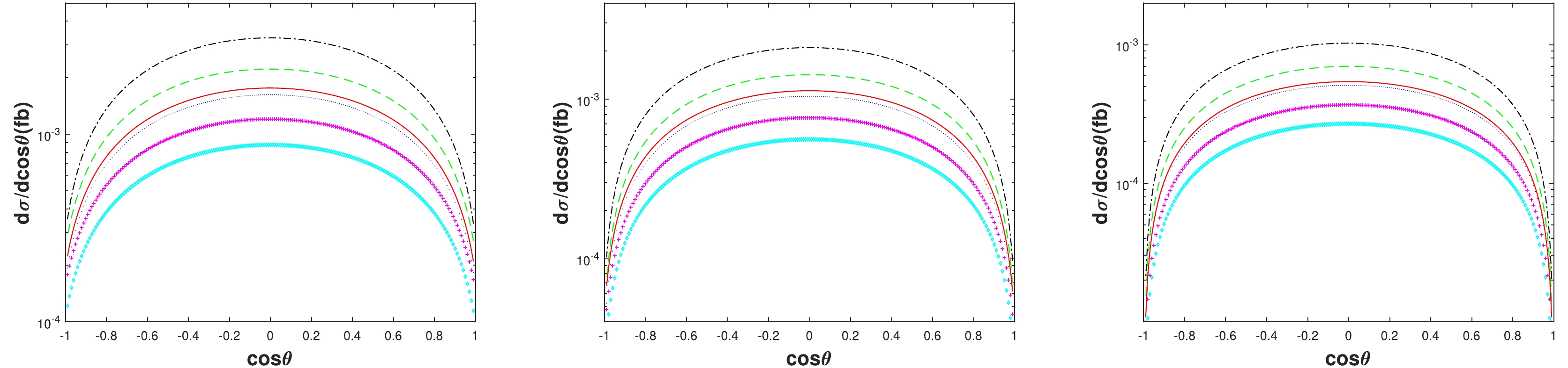

Figure 2.  (color online) The differential angle distributions of cross sections dσ/dcosθ at $ \sqrt{s}=91.1876 $ GeV for $ e^-e^+\to Z^0 \to $$ |(c\bar{c})[n]\rangle+|(c\bar{c})[n']\rangle $. The dash-dotted black line, dotted blue line, dashed green line, solid red line, diamond cyan line, and cross magenta line are for the $ [1]+[1] $, $ [1]+[2] $, $ [1]+[3] $, $ [2]+[1] $, $ [2]+[2] $, $ [2]+[3] $ configurations of the $ |(c\bar{c})[n^3S_1]\rangle+|(c\bar{c})[n'^1P_1]\rangle $ channel (left), the $ |(c\bar{c})[n^1S_0]\rangle+|(c\bar{c})[n'^3P_2]\rangle $ channel (middle), and the $ |(c\bar{c})[n^1S_0]\rangle+|(c\bar{c})[n'^3P_0]\rangle $ channel (right), respectively.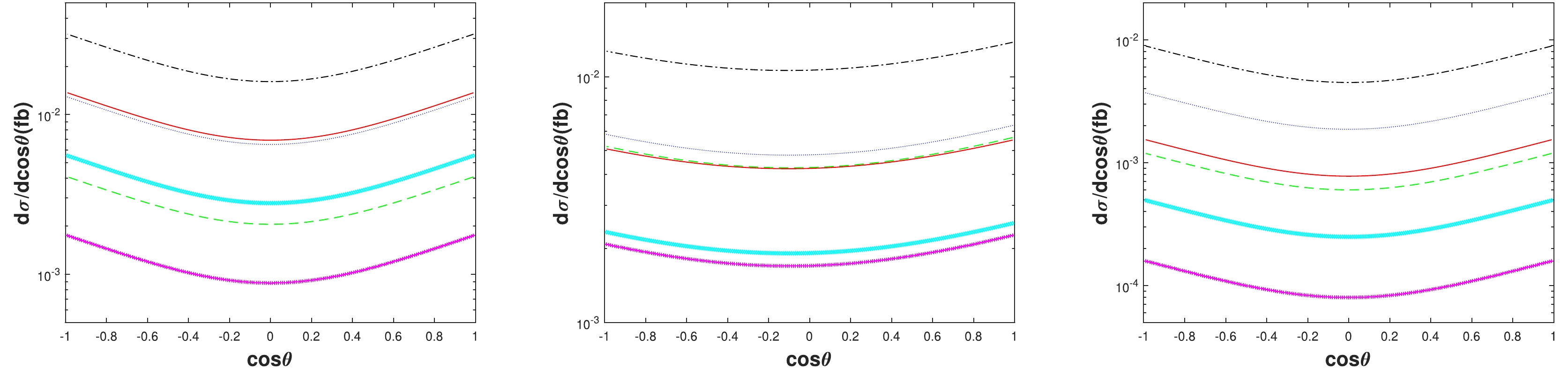

Figure 3.  (color online) The differential angle distributions of cross sections dσ/dcosθ at $ \sqrt{s}=91.1876 $ GeV for the channel $ e^-e^+\to Z^0 \to|(b\bar{b})[n]\rangle+|(b\bar{b})[n']\rangle $. The dash-dotted black line, dotted blue line, dashed green line, solid red line, diamond cyan line, and cross magenta line are for the $ [1]+[1] $, $ [1]+[2] $, $ [1]+[3] $, $ [2]+[1] $, $ [2]+[2] $, $ [2]+[3] $ configurations of the $ |(b\bar{b})[n^1S_0]\rangle+|(b\bar{b})[n'^3S_1]\rangle $ channel (left) and the $ |(b\bar{b})[n^3S_1]\rangle+|(b\bar{b})[n'^3P_2]\rangle $ channel (middle), but for the $ [1]+[1] $, $ [1]+[2] $, $ [1]+[3] $, $ [2]+[2] $, $ [2]+[3] $, $ [3]+[3] $ configurations of the $ |(b\bar{b})[n^3S_1]\rangle+|(b\bar{b})[n'^3S_1]\rangle $ channel (right), respectively.

Figure 4.  (color online) The differential angle distributions of cross sections dσ/dcosθ at $ \sqrt{s}=91.1876 $ GeV for the channel $ e^-e^+\to Z^0 \to|(c\bar{b})[n]\rangle+|(b\bar{c})[n']\rangle $. The dash-dotted black line, dotted blue line, dashed green line, solid red line, diamond cyan line, and cross magenta line are for the $ [1]+[1] $, $ [1]+[2] $, $ [1]+[3] $, $ [2]+[2] $, $ [2]+[3] $, $ [3]+[3] $ configurations of the $ |(c\bar{b})[n^3S_1]\rangle+|(b\bar{c})[n'^3S_1]\rangle $ channel (left), but for the $ [1]+[1] $, $ [1]+[2] $, $ [1]+[3] $, $ [2]+[1] $, $ [2]+[2] $, $ [2]+[3] $ configurations of the $ |(c\bar{b})[n^3S_1]\rangle+|(b\bar{c})[n'^3P_2]\rangle $ channel (middle) and $ |(c\bar{b})[n^1S_0]\rangle+|(b\bar{c})[n'^3S_1]\rangle $ channel (right), respectively.

To get reliable results in LO calculation, we should consider the main uncertainty sources of the cross sections carfully. For values of the input parameters, the fine-structure constant α, the Weinberg angle $ \theta_W $, the Fermi constant $ G_F $, the mass and width of the $ Z^0 $ boson are relatively precise. The non-perturbative matrix elements are an overall factor when the quark mass is fixed. In the following, we probe the uncertainties caused by masses of constituent heavy quarks, and the running coupling constant $ \alpha_s(\mu) $ which is related to the renormalization scale μ.

The uncertainties of total cross sections caused by the varying quark masses have been presented in Tables 2-4 for the production of the double higher excited charmonia, the double higher excited bottomonia, and the higher excited $ B_c $ pair, respectively. We adopt the mass deviations of 0.1 GeV for $ m_c $ (changing about 7%) and 0.2 GeV for $ m_b $ (changing about 4%). Here, the effects of uncertainties of the radial wave function at the origin $ R_{|(Q\bar{Q})[nS]\rangle}(0) $ and its first derivative at the origin $ R'_{|(Q\bar{Q})[nP]\rangle}(0) $ induced by the varying quark masses are also taken into consideration. The uncertainties from the radial wave function at the origin and its first derivative at the origin induced by varying quark masses have been calculated in our previous work in the BT-potential model [26], which we display them explicitly in Table 1. It is shown that a 7% change in the charm quark mass can bring about a correction of up to 20% in the total cross section.

In Figs. 5-7, we present total cross sections σ as a function of the renormalization scale μ at $ \sqrt{s}=91.1876 $ GeV for the production of the double higher excited charmonia, the double higher excited bottomonia, and the higher excited $ B_c $ pair, respectively. It is shown that all the cross sections decrease as the renormalization scale μ increases. The NLO corrections might improve the μ dependence.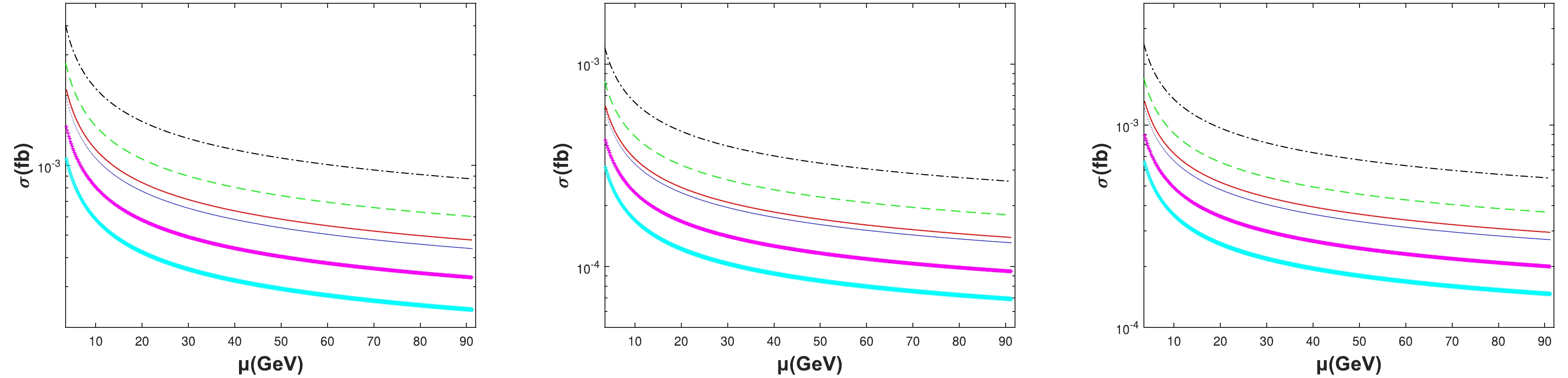

Figure 5.  (color online) The total cross sections σ as a function of the renormalization scale μ at $ \sqrt{s}=91.1876 $ GeV for the channel $ e^-e^+\to Z^0 \to|(c\bar{c})[n]\rangle+|(c\bar{c})[n']\rangle $. The dash-dotted black line, dotted blue line, dashed green line, solid red line, diamond cyan line, and cross magenta line are for the $ [1]+[1] $, $ [1]+[2] $, $ [1]+[3] $, $ [2]+[1] $, $ [2]+[2] $, $ [2]+[3] $ configurations of the $ |(c\bar{c})[n^3S_1]\rangle+|(c\bar{c})[n'^1P_1]\rangle $ channel (left), $ |(c\bar{c})[n^1S_0]\rangle+|(c\bar{c})[n'^3P_2]\rangle $ channel (middle), and the $ |(c\bar{c})[n^1S_0]\rangle+|(c\bar{c})[n'^3P_0]\rangle $ channel (right), respecttively.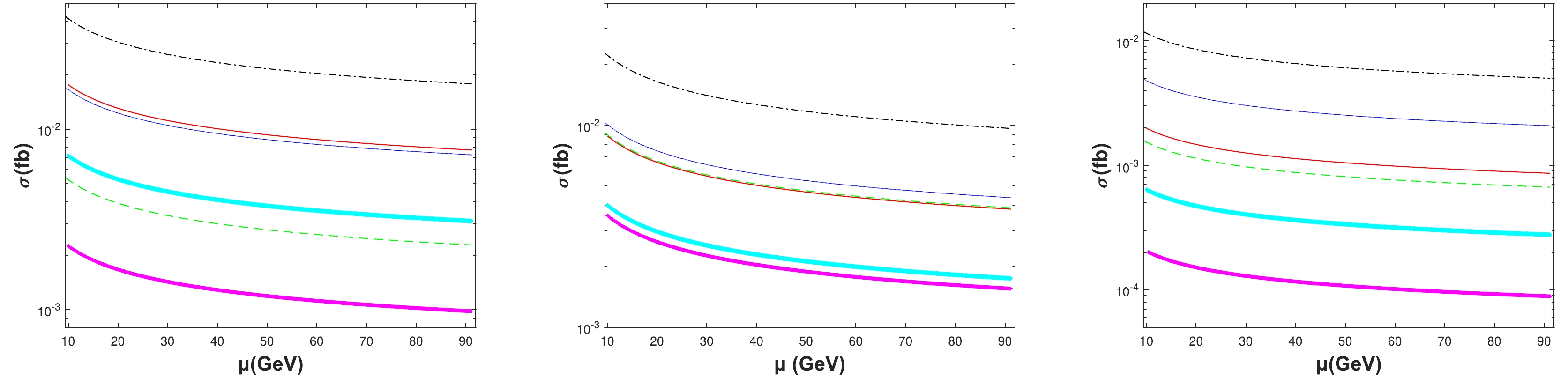

Figure 6.  (color online) The total cross sections σ as a function of the renormalization scale μ at $ \sqrt{s}=91.1876 $ GeV for the channel $ e^-e^+\to Z^0 \to|(b\bar{b})[n]\rangle+|(b\bar{b})[n']\rangle $. The dash-dotted black line, dotted blue line, dashed green line, solid red line, diamond cyan line, and cross magenta line are for the $ [1]+[1] $, $ [1]+[2] $, $ [1]+[3] $, $ [2]+[1] $, $ [2]+[2] $, $ [2]+[3] $ configurations of the $ |(b\bar{b})[n^1S_0]\rangle+|(b\bar{b})[n'^3S_1]\rangle $ channel (left) and $ |(b\bar{b})[n^3S_1]\rangle+|(b\bar{b})[n'^3P_2]\rangle $ channel (middle), but for the $ [1]+[1] $, $ [1]+[2] $, $ [1]+[3] $, $ [2]+[2] $, $ [2]+[3] $, $ [3]+[3] $ configurations of the $ |(b\bar{b})[n^3S_1]\rangle+|(b\bar{b})[n'^3S_1]\rangle $ channel (right), respectively.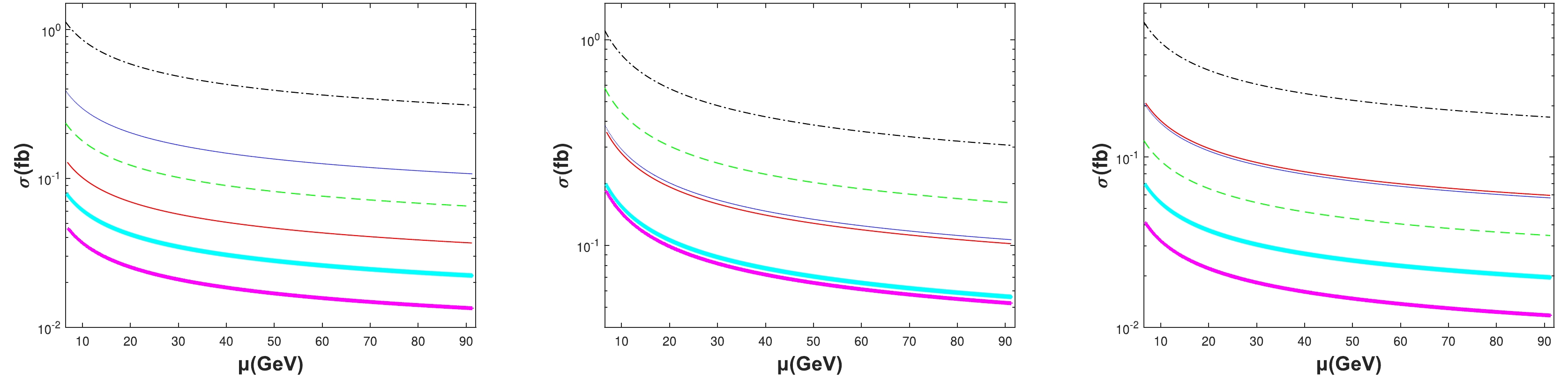

Figure 7.  (color online) The total cross sections σ as a function of the renormalization scale μ at $ \sqrt{s}=91.1876 $ GeV for the channel $ e^-e^+\to Z^0 \to|(c\bar{b})[n]\rangle+|(b\bar{c})[n']\rangle $. The dash-dotted black line, dotted blue line, dashed green line, solid red line, diamond cyan line, and cross magenta line are for the $ [1]+[1] $, $ [1]+[2] $, $ [1]+[3] $, $ [2]+[2] $, $ [2]+[3] $, $ [3]+[3] $ configurations of the $ |(c\bar{b})[n^3S_1]\rangle+|(b\bar{c})[n'^3S_1]\rangle $ channel (left), but for the $ [1]+[1] $, $ [1]+[2] $, $ [1]+[3] $, $ [2]+[1] $, $ [2]+[2] $, $ [2]+[3] $ configurations of the $ |(c\bar{b})[n^3S_1]\rangle+|(b\bar{c})[n'^3P_2]\rangle $ channel (middle) and $ |(c\bar{b})[n^1S_0]\rangle+|(b\bar{c})[n'^3S_1]\rangle $ channel (right), respectively.

In the present work, we systematically study the production of a pair of higher excited charmonia, a pair of higher excited bottomonia, and the higher excited $ B_c $ pair in $ e^+e^-\to Z^0\to |(Q\bar{Q^\prime})[n]\rangle+ |(Q^\prime\bar{Q})[n']\rangle\; (Q,Q^\prime=c,b\; \text{quarks}) $ within the NRQCD factorization framework, where $ [n] $ or $ [n'] $ represents the color-singlet Fock states $ [n^1S_0], \; [n^3S_1], \; [n^1P_1] $, and $ [^3P_J] $ ($ n=1,2,3;J=0,1,2 $). The differential angle distributions of cross sections $ d\sigma/dcos\theta $ are studied for a sound estimation at the future super Z factory, which are shown in Figs. 2-4 for double higher excited charmonia, double higher excited bottomonia, and the higher excited $ B_c $ pair, respectively.

In Tabs. 2-4, it is found that the production rates of the higher excited $ B_c $ pair are roughly two order of magnitude larger than those of the double higher excited charmonia in the same $ [n]+[n^\prime] $ configuration, and are roughly one order of magnitude larger than those of the double higher excited bottomonia in the same $ [n]+[n^\prime] $ configuration. The uncertainties caused by the varying quark masses are also discussed in Tabs. 2-4. It is shown that a 7% change in the charm quark mass can bring a correction of up to 20% in the total cross section. We also present the dependence of total cross sections on the renormalization scale μ in Figs. 5-7. The cross sections always decrease as μ increases.

Our calculation shows that sizable events of the double higher excited heavy quarkonium (principal quantum number $ n=2,3 $) can be produced in the future super Z factory via the process $ e^+e^-\to Z^0 \to |(Q\bar{Q^\prime})[n]\rangle+ |(Q^\prime\bar{Q})[n']\rangle\; (Q,Q^\prime=c,b\; \text{quarks}) $. The future super Z factory should be a good platform to study the exclusive production of the higher excited heavy quarkonium pair. Moreover, since most of these higher excited states would decay into the ground states, we need to take these higher excited states into carful consideration for a sound estimation in our study of the production of the ground states.