Deep Learning to Improve the Sensitivity of Higgs Pair Searches in the 4b Channel at the LHC

The Standard Model (SM) is currently the most successful theoretical framework for describing fundamental particles and their interactions, with the Higgs particle being the core of the model. The Higgs field, through the Higgs mechanism, breaks the Electroweak symmetry spontaneously and explains how fundamental particles acquire mass. Since the discovery of the 125 GeV Higgs particle by the ATLAS and CMS experiments in 2012 [1, 2], precise measurements of the properties of the Higgs, including the determination of its mass, spin, parity, interactions with other particles and Higgs self-coupling, are among the most important tasks in particle physics and provides an essential test of the SM. Despite the great success of the SM, there are still phenomena that cannot be explained in SM, such as the existence of dark matter, the nonzero mass of neutrinos, and the matter-antimatter asymmetry etc. These phenomena suggest the existence of the physics beyond the SM (BSM), and the discovery of the Higgs particle has opened a window for exploring new physics. Any deviation between the measured properties of the Higgs particle and the predictions of the SM would be crucial for us to explore the physics beyond the SM.

Currently, the ATLAS and CMS experiments have already performed various measurements about the Higgs. The mass of the Higgs has been precisely measured by both experiments [3, 4]. The width of the Higgs has also been precisely measured through the off-shell effect [5, 6] which was originally thought not possible at hadron collider. All major production modes and decay channels of the Higgs have been measured [6, 7] with the overall signal strength in agreement with the SM predictions. From these measurements, the interactions of the Higgs with other SM particles can be extracted which are crucial to test the Higgs mechanism.

Measurement of the Higgs self-coupling [8–17] is also an important task in probing the properties of the Higgs boson. The Higgs self-coupling determines the shape of the Higgs potential, which is crucial for electroweak symmetry breaking [18, 19]. In the SM, the Higgs potential is expressed as:

with

where $ v=\sqrt{-\mu^2/\lambda} $ is the vacuum expectation value (vev) determined from the potential. The potential for H after the electroweak symmetry breaking can be expressed as

where $ \lambda_{HHH}=\lambda_{HHHH}=\dfrac{m_H^2}{2v^2} $ represent the trilinear and quartic Higgs self-couplings. It is clear that in the SM, the Higgs self-couplings are fully determined by the mass and vev of the Higgs which have been measured with a high precision. Any deviation from the SM prediction indicates the presence of new physics [20–26]. In this work, we use the kappa framework to parameterize the deviation

where $ \kappa_\lambda $ and $ \kappa_{\lambda,4} $ indicate the deviations in trilinear and quartic Higgs self-couplings respectively. The Effective Field Theory (EFT) framework provides another powerful and model-independent approach to studying the Higgs self-couplings [27–31].

While this study primarily focuses on the trilinear coupling, the quartic Higgs self-coupling is also important. However, direct measurement of this coupling is extremely challenging due to the extremely small cross section of triple Higgs production at current or near-future colliders such as the LHC or the ILC [32]. Future 100 TeV hadron colliders [33–35] or high-energy muon colliders [36] are considered promising platforms for probing this coupling. Additionally, loop corrections in certain Higgs pair production processes, especially in VBF and VHH channels, can also offer indirect sensitivity to the quartic coupling [32].

Direct measurement of the trilinear Higgs self-coupling relies on the Higgs pair productions [37–49] to which the gluon-gluon fusion (ggF) process provides the dominant contribution at the LHC [50–53]. The Higgs pair production from vector boson fusion (VBF) has also been investigated for the measurement of Higgs self-couplings [18, 54]. In addition to ggF and VBF production of a pair of Higgs, many other processes are considered to probe the Higgs self-coupling including the double Higgs-strahlung process [55], Higgs pair associated with two top quarks [18], Higgs pair plus jets production [56, 57]. These processes have smaller cross sections than ggF production, but they can still contribute to the Higgs self-coupling measurement at future colliders with higher energy and luminosity. Further, the single Higgs production and its decay can also be utilized to measure the Higgs self-coupling through its contributions at loop level [58–65]. On the other hand, the Higgs pair production can be significantly altered in extended Higgs sectors where the Higgs pair is produced resonantly [66–72]. The studies of the Higgs pair production can help probing the scalar potential in these models, e.g. xSM [73–76], 2HDM [77–82] and MSSM [83]. However, in this work, we will focus on the non-resonant production of Higgs pair and leave the resonant production to future work.

Both ATLAS and CMS have conducted studies on the Higgs pair production process. In the ATLAS analysis, the decay channels $ HH \rightarrow b\bar{b}b\bar{b} $ [84], $ HH \rightarrow b\bar{b}\tau^+\tau^- $ [85], and $ HH \rightarrow b\bar{b}\gamma\gamma $ [86] were examined. The results indicate that the $ \kappa_{\lambda} $ is constrained to the range $ (-0.6, 6.6) $ after combining all these channels [87]. In the CMS analysis, the decay channels $ HH \rightarrow b\bar{b}ZZ^* $ [88], $ HH \rightarrow \text{Multilepton} $, $ HH \rightarrow b\bar{b}\gamma\gamma $ [89], $ HH \rightarrow b\bar{b}\tau^+\tau^- $ [90] and $ HH \rightarrow b\bar{b}b\bar{b} $ [91] were analyzed. The combined results show that the $ \kappa_{\lambda} $ value is constrained to $ (-1.24, 6.49) $ [7]. Future colliders are expected to significantly improve the measurement precision under higher center-of-mass energy and integrated luminosity. The HL-LHC [92–95] is expected to have a precise measurement of the Higgs self-coupling $ \kappa_{\lambda} = 1.0^{+0.48}_{-0.42} $, while the HE-LHC [96] and FCC-hh [97–100] are projected to achieve a precision of 5% on the Higgs self-coupling. The future lepton collider can also probe the Higgs self-coupling with about 20% precision from FCC-ee [101, 102], ILC [103, 104] as well as multi-TeV muon collider [105–108].

The Higgs boson predominantly decays into $ b\bar{b} $, with a branching ratio of approximately 58% in the SM. Among all possible decay channels, the $ 4b $ final state constitutes the largest fraction (about 33.6%) for a Higgs pair system [109], making it a promising channel for investigation. The current constraints on the Higgs self-coupling are however relatively broad from $ 4b $ channel $ \kappa_\lambda\in(-3.3, 11.4) $ [87], which is weak compared with other channels and mainly limited by the complex background at the LHC. Improving the discriminating power between signal and background in $ 4b $ channel will hence significantly enhance the sensitivity. There are already many studies focusing on improving the sensitivity in this channel [110–116]. In this work, we explore the possibility of using machine learning techniques to tackle the challenge in $ 4b $ channel of Higgs pair searches at the LHC.

The amount of data generated at colliders is enormous, and machine learning (ML) is particularly well-suited for handling such large-scale datasets [117–119]. There have been various ML applications in particle physics [120, 121], such as jet-tagging [122–125] including CNN based on image data [126–129], GNN based on graph data [130–132], ParticleNet and Energy Flow Network based on particle clouds [133–136], and the current state-of-the-art (SOTA) Transformer-based model, Particle Transformer (ParT) [137–141]. Similarly, for the measurements of Higgs self-coupling, ML techniques are also used [115, 116, 142–144]. Additionally, there are studies that investigate the performance of different machine learning algorithms in Higgs self-coupling measurement [145–147].

For the $ HH \rightarrow b\bar{b}b\bar{b} $ channel, different machine learning architectures have been applied. For instance, Ref. [115] employing a DNN architecture demonstrated that, with $ {\cal{L}}=3000\,{\rm{fb}}^{-1} $ at HL-LHC, the Higgs self-coupling can be constrained within the range $ \kappa_\lambda\in(-0.8, 6.6) $ at 68% CL. A more recent work [116] utilizing a Transformer model achieved a constraint of \(\kappa_{\lambda} \in (-1.56, 7.57)\) at 95% CL with $ {\cal{L}}=300\,{\rm{fb}}^{-1} $ at the LHC. Another transformer-based model is also used for the resonant Higgs pair production study with $ 4b $ final states [148]. Considering the excellent performance of ParT in jet tagging tasks [137], in this work, a modified version of ParT including entire event information as input for event classification will be used to improve the sensitivity on the Higgs self-coupling through $ HH\to b\bar{b}b\bar{b} $ channel. However, we need to emphasis that the analysis included in this study demonstrates the effectiveness of not only the transformer structure on the event selection, but also the end-to-end analysis utilizing the event-level information.

This paper is organized as follows. In Sec. II, we briefly describe all the processes we will consider in this work. In Sec. III, after the introduction of the structure of ParT, we will discuss the modification we will made and the details of the training process. The performance of the modified model on event classification will also be presented. In Sec.IV, we present the results on the Higgs self-coupling measurement with a comparison among different methods. The interpretability of the model is also discussed at the end of this section. Finally, we summarize in Sec.V.

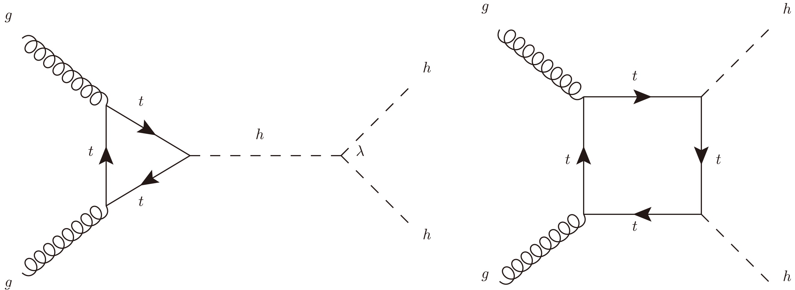
For the Higgs self-coupling measurement, we focus on the non-resonant gluon-gluon fusion (ggF) production of Higgs pair[149–151], with both Higgs decays into b-quark pair, which contains, at leading order (LO), the contributions from triangle and box diagrams as well as the interference between them. The representative Feynman diagrams are shown in Fig. 1. The triangle diagrams depend on both the trilinear Higgs self-coupling and Yukawa couplings, while the box diagrams depend only on the Yukawa couplings of the fermion in the loop. In our simulations, we include the contributions from the third generation quarks, but with fixed Yukawa coupling at corresponding SM value. On the other hand, the trilinear Higgs self-coupling is allowed to be different with the SM value. The total Higgs pair production cross section at given energy will be a quadratic function of $ \kappa_\lambda $, and is given as at both $ \sqrt{s}=13\,\rm TeV $ and $ \sqrt{s}=14\,\rm TeV $:

Figure 1.  The leading-order Feynman diagrams of the di-Higgs production in the SM.

where the first term depending on $ \kappa_\lambda^2 $ in each line is the pure triangle contributions, the last term without any dependence on $ \kappa_\lambda $ comes from the box diagrams, while the middle term with linear dependence on $ \kappa_\lambda $ comes from the interference effects between the triangle and box diagrams. The cross section is further normalized according to the higher order k-factor given in [115] which is about 2.4 for $ \kappa_\lambda=1 $ and varies by 35% for $ \kappa_\lambda\in[-5, 12] $ ranging from $ k\approx 2.28 $ at $ \kappa_\lambda=2 $ to $ k\approx 3.12 $ at $ \kappa_\lambda=5 $. The Higgs pair production cross sections for different choices of $ \kappa_\lambda $ at different energies are shown in Fig. 2.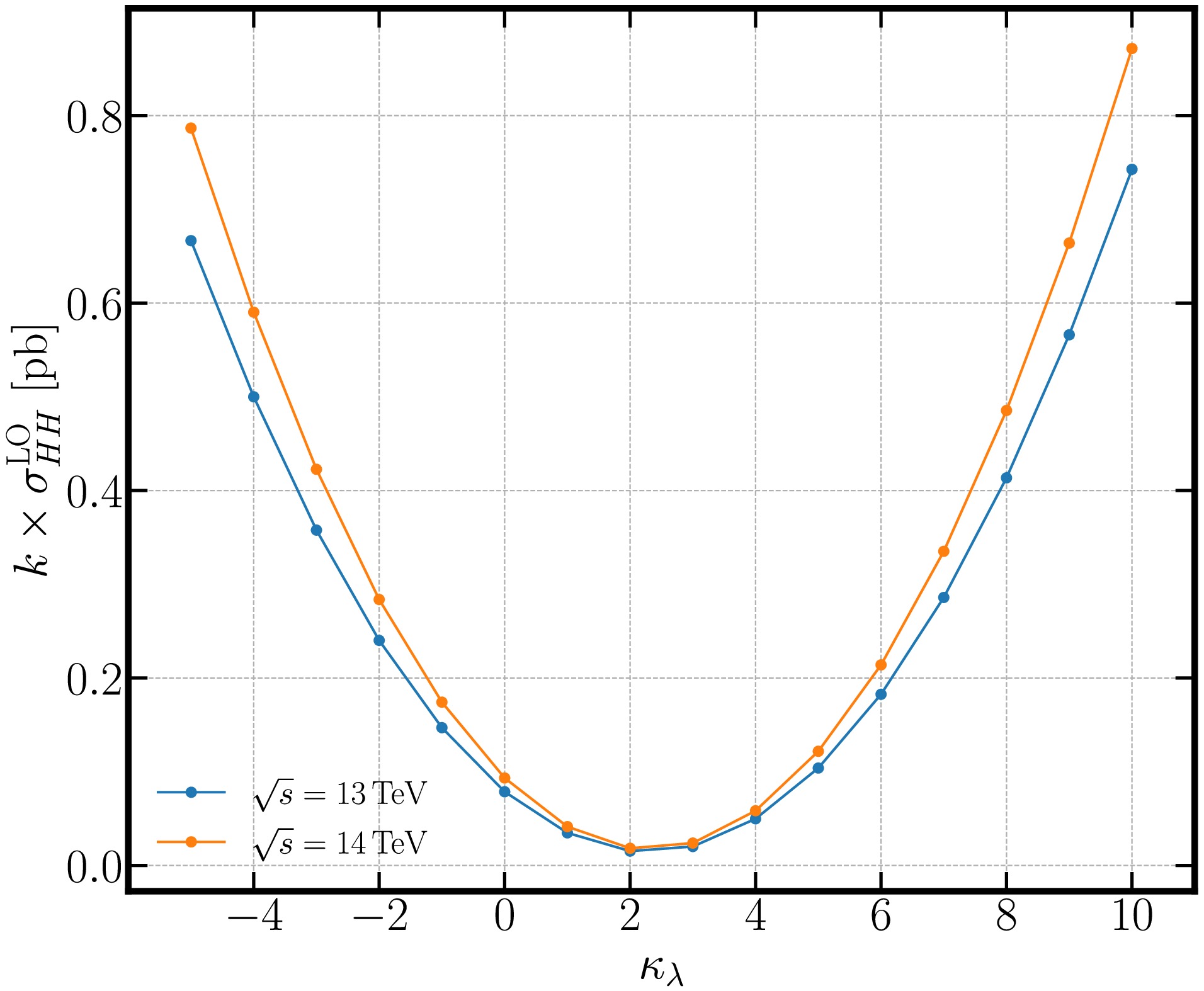

Figure 2.  (color online) The Higgs pair production cross section as function of $ \kappa_\lambda $ at the LHC ($ \sqrt{s}=13\,\rm TeV $ and 14 TeV), assuming all other couplings are fixed, with higher order correction k-factor included.

For the backgrounds, we will mainly focus on the processes containing multi b-quarks and/or multi-jets. In our analysis, the main backgrounds are the QCD production of four b quarks ($ 4b $) as well as two b quarks together with two light quarks ($ 2b2j $). Other than these two major backgrounds, we also consider the production of b-quarks from the decay of Z boson, Higgs, and top quark. In Table 1, we list all signal (given with $ \kappa_\lambda = 1 $) and background processes considered in this analysis together with their cross section at LO at both $ \sqrt{s}=13\,\rm TeV $ and $ \sqrt{s}=14\,\rm TeV $. For the signal, as well as $ t\bar{t} $, $ 4b $ and $ 2b2j $ background processes, the NLO k-factors are also listed [115, 152–155].

Process	$ \sigma^{\rm LO} $ [fb]		k-factor
	$ \sqrt{s}=13 $ TeV	$ \sqrt{s}=14 $ TeV
$ HH $	$ 1.446\times 10^1 $	$ 1.723\times 10^1 $	2.4
$ b\bar{b}b\bar{b} $	$ 2.465\times 10^6 $	$ 2.840\times10^6 $	1.6
$ b\bar{b}jj $	$ 5.673\times 10^8 $	$ 6.470\times10^8 $	1.3
$ t\bar{t} $	$ 5.058\times 10^5 $	$ 5.968\times10^5 $	1.5
$ t\bar{t}b\bar{b} $	$ 3.614\times10^3 $	$ 4.472\times10^3 $	−
$ t\bar{t}H $	$ 3.997\times 10^2 $	$ 4.794\times 10^2 $	−
$ b\bar{b}H $	$ 4.746\times 10^1 $	$ 5.496\times 10^1 $	−
$ ZZ $	$ 9.317\times10^3 $	$ 1.026\times10^4 $	−
$ ZH $	$ 5.799\times10^2 $	$ 6.422\times10^2 $	−

Table 1.  All processes considered in this work, with the LO cross section at $ \sqrt{s}=13\,\rm TeV $ and $ \sqrt{s}=14\,\rm TeV $. The k-factor is the factor to account for the NLO correction for the major backgrounds $ 4b $, $ 2b2j $ and $ t\bar{t} $ processes, and higher order corrections for the signal $ HH $ at $ \kappa_\lambda=1 $.

The events for both signal process with possible different values of $ \kappa_\lambda $ and background processes are simulated by ${\mathtt{MadGraph}}$ [156] with both $ \sqrt{s}=13\,\rm TeV $ and $ \sqrt{s}=14\,\rm TeV $. To increase the simulation efficiency, we use a moderate parton-level basic cuts: $ p_T^{j,b} > 20\,{\rm{GeV}} $, $ |\eta^{j,b}|<4 $. The ${\mathtt{Pythia}}$ [157] is used for the hadronization and showering followed by the detector simulation by ${\mathtt{Delphes}}$ [158]. ${\mathtt{FastJet}}$ [159] is further linked to reconstruct the Jets from the particle-flow output from ${\mathtt{Delphes}}$ using anti-$ k_t $ algorithm [160] with two different values of $ \Delta R $, 0.5 for a slim jet originated from quarks/gluon, 1.0 for a fat jet originated mainly from heavier objects, e.g. Higgs, W/Z boson, top quarks.

In this study, instead of working on the individual objects (jets, charged leptons, photons etc.) within an event, we investigate the possibility of directly working on the whole event. The Particle Transformer (ParT) [137] is the state-of-the-arts (SOTA) object tagging machine learning (ML) algorithm, which was trained on a 10-label-classification task. By implementing ParT, we could in principle tag the Higgs, top, W/Z boson as a fat jet in the events, and then combine them to extract the event of signal (Higgs pair) from other background processes (containing top quark, W/Z boson etc.). Although, the individual object reconstruction efficiency is sufficient, relying on reconstructed individual heavy objects inside one events may suffer from the combinatorial problem which can heavily reduce the sensitivity, especially for $ HH\to b\bar{b}b\bar{b} $ case where the four b-jets in the final states are indistinguishable and there are 6 combinations of these b-jets to form one Higgs pair candidate. Hence, we explore the possibility of training on the information of entire event which can be treated as a single extremely fat jet. Consequently, the ParT framework can still be used with minor modification in the event classification task. In the following, we will first briefly introduce the main features of ParT. Then the training details in our setup will be presented. The performance on the event classification is also discussed. To avoid confusion with the original ParT model, we will refer to the ParT working on the entire event in our setup as Event Transformer (EvenT). However, we also want to emphasis that the analysis presented in this work can be performed based on any kind of algorithms other than Transformer. The focus here is the possibility of an end-to-end event level analysis.

The ParT [137] is basically a classification model based on the Transformer architecture [161] which is a deep learning model originally designed for natural language processing (NLP) tasks. The core of Transformer is the self-attention mechanism, which establishes relationships among all elements in the input sequence, rather than being limited to local information like CNN. By computing the attention weight matrix, Transformer can capture global information. Due to the advantages of this mechanism, Transformer has demonstrated powerful performance across multiple domains.

The structure of ParT is shown in Fig. 3. The model receives two sets of inputs: particles which include the features (kinematics, PID, trajectory displacment etc.) of each single object (tracks, charged leptons etc.) and interactions which indicate the relationships between two objects. In ParT, there are mainly 4 such relationships:

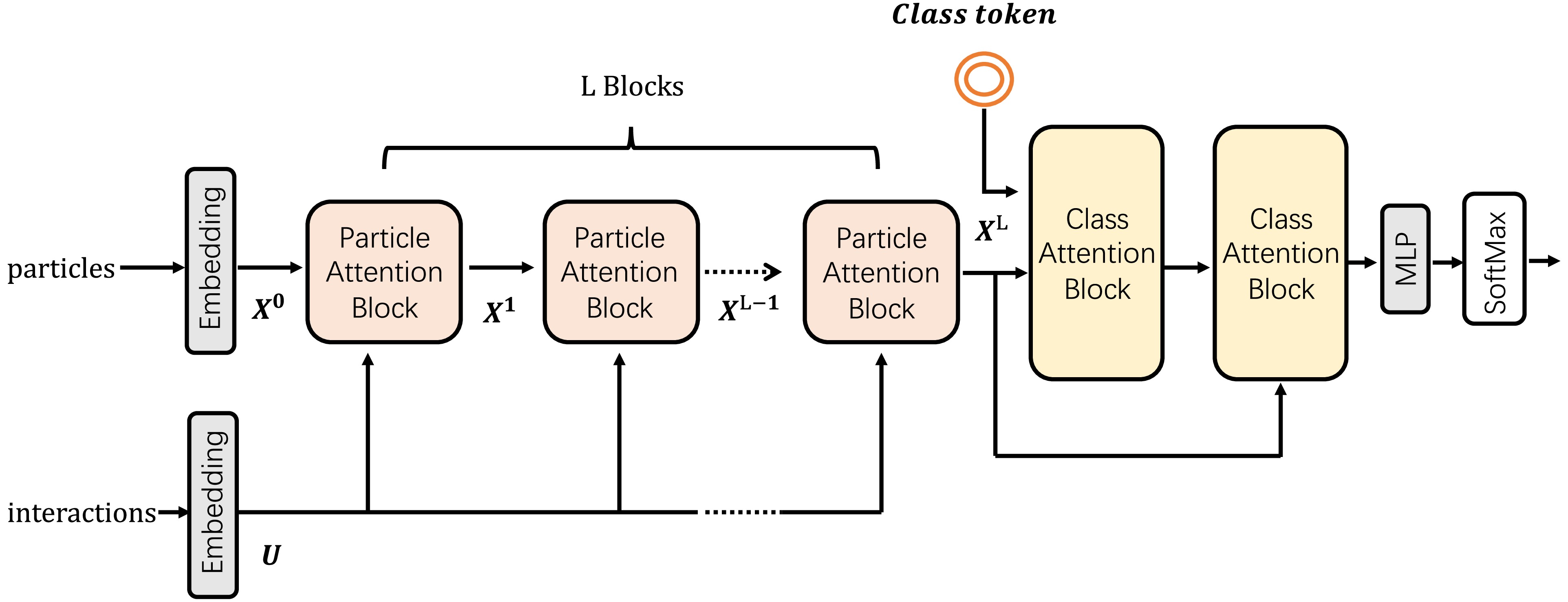
Figure 3.  (color online) The ParT Model Architecture.

where $ y,\phi $ are the rapidity and azimuthal angle of the individual object respectively. $ p_T $ is the corresponding magnitude of the transverse momentum. Then the inputs are passed through the intermediate layers consisting of Particle Attention Blocks and Class Attention Blocks. Compared to the traditional Transformer, ParT introduces, in the Particle Attention Block, new attention mechanism referred as particle multihead attention (P-MHA) where the interactions are included in the attention calculation:

where X includes the particles features, U contains features of the interactions between objects. $ W_i^j $ and $ b_i^j $ are trainable parameters. Including the interactions U in the attention calculation enables the model to better capture the relationships between particles and enhance the expressiveness of the attention mechanism. $ {\cal{A}}_i $ is the attention weight matrix of which each element represents the attention score of each pair of input particles.

The Class Attention Block shares a similar architecture with the Particle Attention Block but differs in two main aspects: it uses the standard Multi-Head Attention (MHA) mechanism instead of the particle-specific variant, and the MHA takes a global class token as input along with the particle embeddings. The query, key, and value matrices are then computed as:

where $ {\bf{Z}} = [X_{\text{class}}, X_{\rm PAB}] $ is the concatenation of the class token and the particle embedding output from the last Particle Attention Block. The output of the Class Attention Block are then passed to a Softmax layer which produces the probabilities over the classes.

In our setup, the EvenT model receives the information from the whole event as input features. To further facilitate establishing connections among objects within an event, information from jets reconstructed using two different $ \Delta R = 0.5 $ and 1.0, as discussed in last section, is also provided. Hence, the input for EvenT now includes particle features of all objects within one event including tracks, energy deposits, charged leptons, jets and event itself, which extend the dimension of the input substantially. Note that, the orientation of a single event is not important. Further, the interaction features are also extended to include the affiliation relations between different objects in additional original kinematic relations. To avoid the time-issue when loading all inputs, the interaction features are now calculated in advance. The EvenT model is trained from scratch on a dataset with 9 classes listed in Table 1 containing 3 million samples per class. After each training epoch, the model is validated on a separate validation set containing 3 million samples per class, while its final performance is evaluated on an independent test set with an equivalent sample size per class. The model is trained with a batch size of 128 and initial learning rate of 0.001. The learning rate remains constant during the first 70% of training epochs, after which it decays exponentially, reaching 1% of its initial value by the end of training. The number of training epochs is set to 50, and the number of heads in the multi-head attention mechanism is 8.

In general, all processes during the training shall be treated equally. However, for our purpose, we would like to single out the Higgs pair process as much as possible from the other processes among which $ 2b2j $ process has the largest cross section. In order to avoid large contamination from $ 2b2j $ process, unlike ParT which is used for a general purpose jet-tagging task, we adopt a weighted cross-entropy loss function, where the process $ 2b2j $ is assigned with a weight of 70, while all other processes are assigned with a weight of 1. After applying the weighted cross-entropy loss, the probability of miss-classifying $ 2b2j $ events as $ HH $ events is reduced from $ 5.17\times10^{-3} $ to $ 5.26\times10^{-5} $ by two orders of magnitude which dramatically improves the analysis about the Higgs pair process. The measurement uncertainty of the Higgs pair production cross section can be reduced from about 400% to around 200% by such improvement.

Further, as our target is the measurement of $ \kappa_\lambda $, the model is required to work properly on all different value of $ \kappa_\lambda $ in order to obtain the optimal result. As a comparison, we show in Fig. 4 the results of $ HH $ efficiency from training on data set with only $ \kappa_\lambda = 1 $ (blue line) and training on data set containing $ \kappa_\lambda = \{-1,1,4,6,8\} $ (red line). It is clear that for the training using data with only $ \kappa_\lambda = 1 $, the $ HH $ efficiency will dramatically decrease for other value of $ \kappa_\lambda $. The variance of the efficiency can be as large as 40% (from 58% at $ \kappa_\lambda=2 $ to 18% at $ \kappa_\lambda = 3 $). On the other hand, when we include the data with other value of $ \kappa_\lambda $, the $ HH $ efficiency is roughly stable at around 50%. Such performance is hence suitable for the further analysis on the measurement precision about $ \kappa_\lambda $.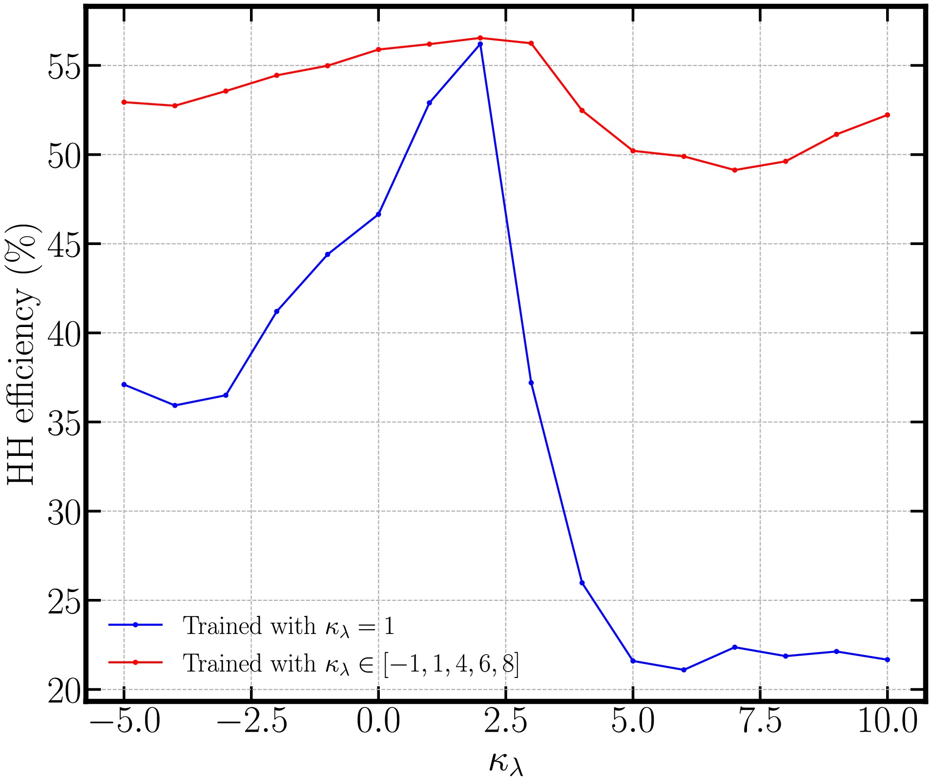

Figure 4.  (color online) $ HH $ efficiency under different $ \kappa_{\lambda} $ values for training containing only $ \kappa_\lambda=1 $ $ HH $ data (blue line) and training containing $ \kappa_\lambda=-1,1,4,6,8 $ $ HH $ data (red line).

In this section, we further demonstrate the classification performance of the model. EvenT is now essentially a multi-class classification model with 9 event categories. For multi-class models, the performance can be evaluated using the confusion matrix, ROC curves and AUC scores.

A confusion matrix is structured as an $ N \times N $ matrix, where N denotes the number of target classes, with rows representing true labels and columns indicating predicted labels, to quantify the performance of the classification model. The confusion matrix can be presented as:

Specifically:

● $ C_{ii} $ represents the probability that an event of true class i is correctly predicted as class i.

● $ C_{ij} $ (for $ i \neq j $) represents the probability that an event of true class i is incorrectly predicted as class j.

The confusion matrix of EvenT on the test set, where the $ HH $ class only includes events with $ \kappa_{\lambda}=1 $, is visualized in the left panel of Fig. 5 where the color intensity indicates the corresponding probabilities.

Figure 5.  (color online) Left: Confusion matrix of the EvenT on 9-class classification task. Right: OvR ROC curves for each class of EvenT and the corresponding AUC. All the results are obtained with the weighted cross-entropy loss.

There are several comments about the confusion matrix in order. First, it is clear from the $ 2b2j $ column, every class has a relatively high efficiency tagging as $ 2b2j $ since we enhance the weight of $ 2b2j $ events during the training as discussed above. Second, as can be seen from the diagonal elements, when not considering the $ 2b2j $ class, the rest classes all have a good self-tagging efficiency. Further, processes similar to each other will form a diagonal block in the tagging efficiency, e.g. $ (ttbb, ttH) $ and $ (ZZ, ZH) $. For our purpose of measuring Higgs pair production process, the first column of the confusion matrix indicates that all other processes have been heavily suppressed while keep a sufficient efficiency of $ HH $ process.

The ROC (Receiver Operating Characteristic) curve and AUC (Area Under Curve) are commonly used metrics for binary classification tasks. They can also be extended to multi-class classification problems for model evaluation. In a binary classification setting with only positive and negative classes, the ROC curve is generated from the True Positive Rate (TPR) and the False Positive Rate (FPR) at various classification thresholds. The AUC is the area under the ROC curve and is used to quantify the overall classification performance.

For multi-class classification tasks, the One-vs-Rest (OvR) strategy can be used to simplify the problem into a series of binary classification tasks, allowing the computation of ROC curves and AUC scores. For each class, it is treated as the positive class while all other classes are treated as the negative class. The right panel of Fig. 5 shows the ROC curves and the corresponding AUC values for each class. For most of the classes, the AUC is around 0.9 indicating a relatively good performance of the EvenT. Further, the AUC for distinguishing $ HH $ process from other processes is about 0.9, this provides a solid foundation for the analysis of the Higgs self-coupling via Higgs pair production in the next section. On the other hand, the information contained in the confusion matrix as well as those OvR ROC curves can be used not only on the $ HH $ analysis, but also on other relevant analysis. In this work, we use the $ HH $ as a benchmark study to demonstrate the effectiveness of the end-to-end analysis based on event-level information especially when involving pairing or other event topology analysis that will reduce the selection efficiency.

Based on the EvenT discussed in the above section, we will consider the measurement of $ \kappa_\lambda $ through the $ HH\to 4b $ channel in this section. The corresponding $ \chi^2 $, which indicates the deviation from the SM case, is constructed according to

where $ i=1,\cdots,9 $ corresponds to all the processes considered in the confusion matrix shown in the left panel of Fig. 5, including: $ HH $, $ tt $, $ ttH $, $ ttbb $, $ Hbb $, $ 4b $, $ 2b2j $, $ ZZ $, and $ ZH $. $ C_{ij} $ represents the elements in the confusion matrix. For $ HH $ process, the dependence of $ C_{11} $ on $ \kappa_\lambda $ is also included as shown in Fig. 4. $ \sigma_i $ denotes the cross section of each process listed in Table 1. Note that $ \sigma_{HH} $ will be a free parameter in the $ \chi^2 $ calculation. In our analysis, we consider the LHC experiment with $ \sqrt{s} = 14\,\rm TeV $ and integrated luminosities of $ {\cal{L}} = 300/3000\,{\rm{fb}}^{-1} $. Based on the above setup, for a fixed value of $ \kappa_\lambda $, the $ \chi^2 $ depends sorely on the corresponding Higgs pair production cross section $ \sigma_{HH} $. Then, the upper limit on the cross section $ \sigma_{HH} $ can be obtained for given $ \kappa_\lambda $ by solving $ \chi^2(\sigma_{HH},\kappa_\lambda)=1 (3.84) $ for 68% (95%) confidence level (CL).

However, as we discussed in above section, the performance of EvenT also depends on the classification threshold. The effect of the threshold on the Higgs pair production measurement is shown in Fig. 6. We can see that the signal efficiency decrease smoothly with the increase of the threshold for both $ \kappa_\lambda=1 $ (solid green line) and $ \kappa_\lambda=5 $ (dashed green line). While the misclassification rate of the dominant background $ 2b2j $ (solid orange line) drops more sharply. Hence, the relative error of measuring the Higgs pair production cross section will decrease with higher threshold as shown by the blue curves in Fig. 6. However, we need to emphasize that when the threshold is close to 1, the events passing the threshold will decrease dramatically. The corresponding analysis hence suffers from large uncertainties. In our analysis, we will use three benchmark thresholds $ p_{\rm th}=0.5,0.7,0.9 $ (indicated by the vertical purple dashed lines in Fig. 6) together with $ p_{\rm th}=0.0 $ where we rely entirely on the raw output of EvenT for the classification.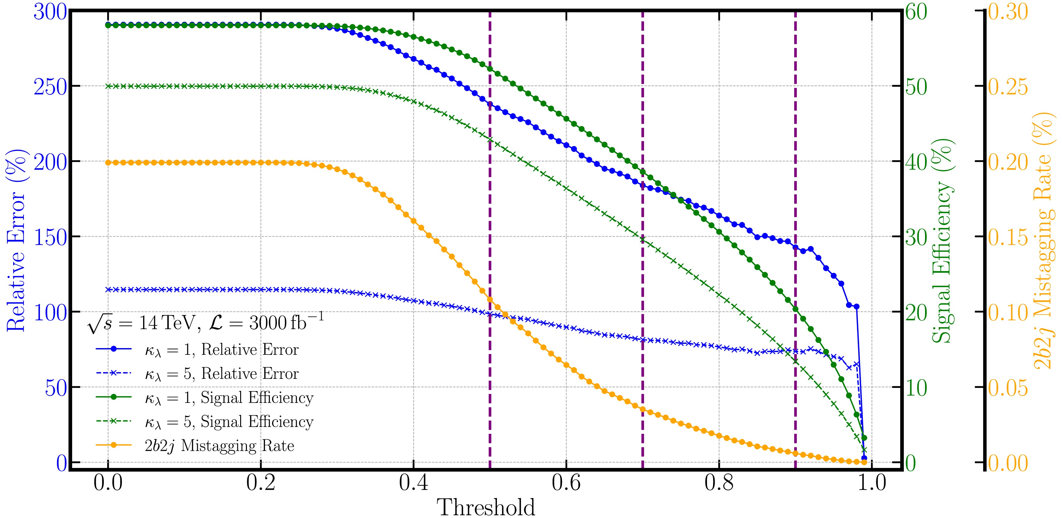

Figure 6.  (color online) Signal efficiency (green lines) and relative error of the Higgs pair production cross-section measurement (blue lines) for $ \kappa_\lambda = 1 $ (solid lines) and $ \kappa_\lambda = 5 $ (dashed lines) at different thresholds. The misclassification rate of the dominant background $ 2b2j $ is also shown in orange.

The upper limits on the Higgs pair production cross section as a function of $ \kappa_\lambda $ obtained from EvenT with different classification thresholds are shown in Fig. 7. The upper limits follow well with the $ HH $ efficiency shown in Fig. 4. The theoretical prediction of the Higgs pair production cross section is also shown in Fig. 7. By comparing the EvenT-derived upper limits with the theoretical prediction, we can extract the constraints on the Higgs self-coupling $ \kappa_\lambda $. At the HL-LHC, $ \sqrt{s}=14\,\rm TeV $ and $ {\cal{L}}=3000\,{\rm{fb}}^{-1} $, the constraint at 68% CL is given as $ \kappa_\lambda \in [-0.25, 5.41] $ for $ p_{\rm th}=0.9 $. The constraints will be a little bit weaker for other choices of the threshold as indicated in Fig. 7.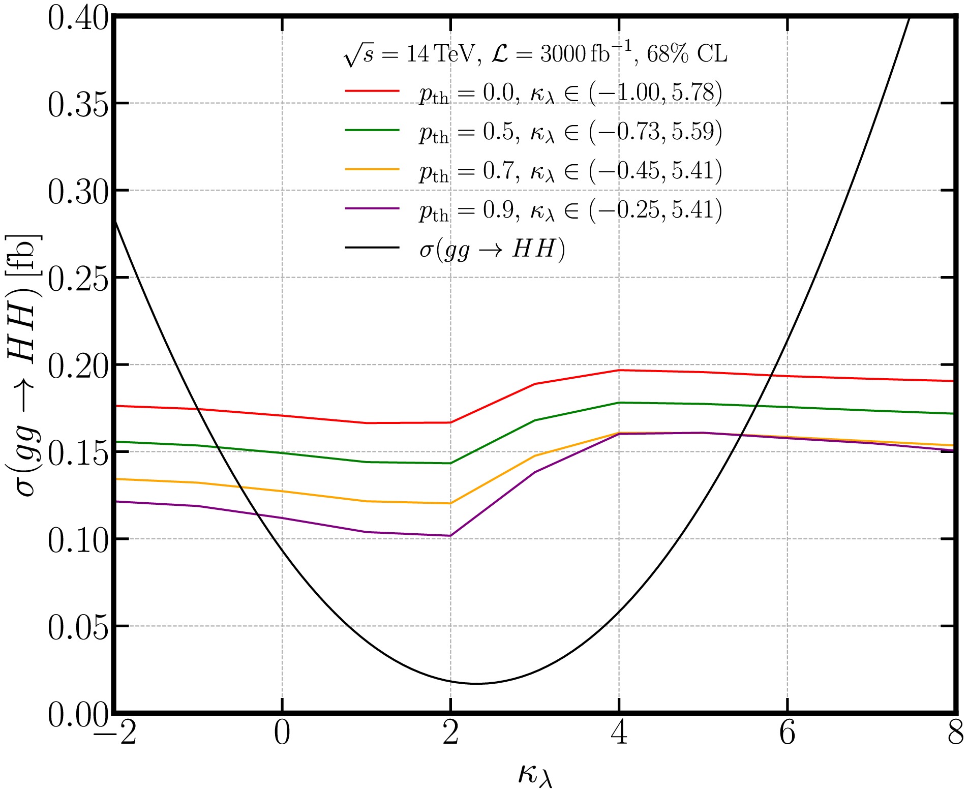

Figure 7.  (color online) Upper limit on the Higgs pair production cross section as a function of $ \kappa_\lambda $ for different classification thresholds $ p_{\rm th} $ (four colored lines) with $ \sqrt{s}=14\,\rm TeV $ and $ {\cal{L}}=3000\,{\rm{fb}}^{-1} $ at the LHC. The Higgs pair production cross section as a function of $ \kappa_\lambda $ is also shown as black line.

As a comparison, we followed the cut-based analysis presented in [84] to single out $ HH\to b\bar{b}b\bar{b} $ events. In this analysis, the events first need to pass several general selections including: requiring at least 4 b-tagged (with tagging efficiency about 77%) jets with $ p_T>40\,{\rm{GeV}} $, and $ |\eta_b|<2.5 $. The four b-jets with the highest $ p_T $ will be used to reconstruct the Higgs pair system. Among the three possible pairings of these four b-jets, the one in which the higher $ p_T $ jet pair has the smallest $ \Delta R $ is used for further analysis. To further suppress the background, $ |\Delta\eta_{HH}|<1.5 $ is also imposed for the two reconstructed Higgs.

Events are further required to satisfy additional selection criteria designed to reduce the background and improve the analysis sensitivity. To suppress the $ t\bar{t} $ background, a top veto cut is needed. The top veto discriminant $ X_{Wt} $ is defined as:

where $ m_W = 80.4\,{\rm{GeV}} $ and $ m_t = 172.5\,{\rm{GeV}} $ are the nominal W boson and top quark mass. $ m_{jj} $ is the invariant mass of two jets that are assumed to come from the W boson decay. Together with one of the leading b-jet, $ m_{jjb} $ represent the invariant mass of the reconstructed top. The $ X_{Wt} $ is then obtained by minimizing over all the combinations of two normal jets and one b-jet. During the minimization, 10% uncertainties are used to approximate the invariant mass resolution. Then events with $ X_{Wt}<1.5 $ are excluded in the analysis.

A discriminant $ X_{HH} $ is defined to further test the compatibility of events with the $ HH\to b\bar{b}b\bar{b} $:

where $ m_{H_1} $ and $ m_{H_2} $ are the masses of the leading and subleading reconstructed Higgs boson candidates, respectively. The reference mass $ 124\,{\rm{GeV}} $ and $ 117\,{\rm{GeV}} $ are obtained from the $ m_{H_1} $ and $ m_{H_2} $ distribution from the simulation [84]. Note that, when calculating $ X_{HH} $, 10% uncertainties are also used for the reconstructed invariant masses. Events with $ X_{HH} < 1.6 $ are considered as $ HH\to b\bar{b}b\bar{b} $ signal. All above selections are used on our events including signal events with different $ \kappa_\lambda $ as well as all backgrounds including the most important QCD backgrounds $ 4b $ and $ 2b2j $ as well as $ tt $, $ ttbb $, $ ttH $, $ bbH $, $ ZZ $, $ ZH $ as listed in Table 1. The results are shown in Fig. 8 and will be discussed in the following section.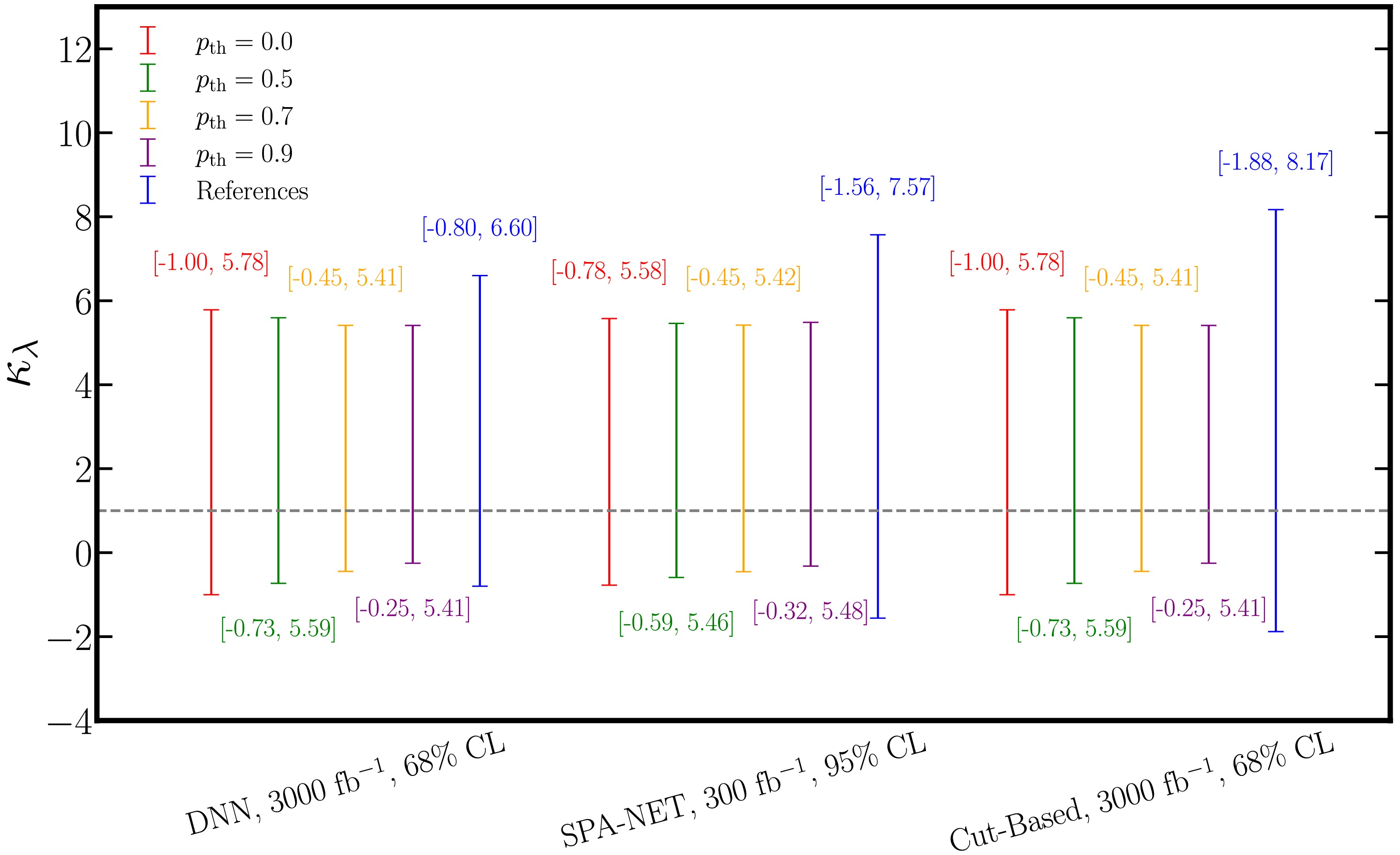

Figure 8.  (color online) The comparison of the constraints on $ \kappa_\lambda $ with three benchmark studies.

To demonstrate the performance of EvenT, we compare the results obtained from the EvenT-based analysis with those from a cut-based analysis using kinematic variables discussed above, as well as with two ML-based studies, one using DNN [115], the other using SPA-NET [116]. The comparison are shown in Fig. 8.

The studies in [115] employs a DNN-based model to single out the Higgs pair signals where they also include comprehensive background studies. The DNN model contains two fully connected hidden layers with 250 hidden nodes with ${\mathtt{ReLU}}$ activation function. To prevent overfitting, ${\mathtt{Dropout}}$ layer is added between the two hidden layers which randomly drop 30% of the nodes during training. The results are given at 68% CL with an integrated luminosity of $ 3000\,{\rm{fb}}^{-1} $ at the HL-LHC. The comparison is shown in the left group of Fig. 8. It is clear that when $ \kappa_\lambda > 0 $, even we do not deal with the threshold to enhance the sensitivity, the constraint from EvenT is stronger than that from the DNN method. While for the negative side, as we only include one negative value in the training $ \kappa_\lambda = -1 $, without imposing the threshold, the constraint from EvenT is a bit weaker than that from the DNN method. However, when we include a moderate threshold to enhance the sensitivity, the result becomes better than that of DNN.

SPA-NET is also an attention-based model [162–164] that employs a stack of transformer encoders to embed input features. These embeddings are then used for jet assignment and event classification via a symmetric tensor attention module, which preserves the permutation symmetry inherent to the input data. The SPA-NET has also been used in the $ HH\to b\bar{b}b\bar{b} $ analysis in [116] where the architecture is used both in pairing of the b-jets into two Higgs as well as in signal-background discrimination. However, the analysis in [116] considered only the $ 4b $ background. Hence, the comparison is made by including only $ 4b $ background in EvenT analysis. The results are shown in the middle group of Fig. 8 which are given at 95% CL with $ 300\,{\rm{fb}}^{-1} $ luminosity at the LHC. It is clear that, with only $ 4b $ background, the results from EvenT are better than that from SPA-NET from both side even without imposing any threshold. Note that both SPA-NET and EvenT are based on Transformer framework, the results hence demonstrate the effectiveness of the event-level analysis.

The comparison with the cut-based analysis discussed above is also presented in the right group of Fig. 8. Note that the cut-based analysis and EvenT-based analysis are performed on the same set of testing data. The constraints on $ \kappa_\lambda $ are given at 68% CL with $ 3000\,{\rm{fb}}^{-1} $ at 14 TeV. It is clear that, the EvenT result is already better than that from the cut-based analysis without imposing any threshold to enhance the sensitivity. With stronger threshold in the classification, the result from EvenT becomes much stronger than that from the general cut-based analysis which clearly demonstrates the advantage of the ML models in the analysis.

Before we conclude, in this section, we also would like to discuss the interpretability of the EvenT model to understand the internal connections of the model. As we have mentioned previously, the outstanding performance of Transformer based models is mainly attributed to the attention mechanism. Hence, we will mainly focus on the visualization of the attention mechanism of the EvenT model following the method in [165] using the attention matrix in Eq. (12), especially in our case where the inputs contain the information from the whole event instead of fully reconstructed objects. We visualized the attention scores from the first attention head of the last particle attention block. The results are shown in Fig. 9 which presents the attention score (element of the attention matrix) of $ HH $ (upper panels) and $ 2b2j $ (lower panels) processes. As a comparison, we present the attention matrix after (left panels) and before (right panels) training together. In order to make the plot clear, we ignore the attention score that is lower than 0.01. It is clear that the attention score is more concentrated for both $ HH $ and $ 2b2j $ processes with the training which strongly indicates that the model does learn the important relationship between particles. Further, the model will pay attention to different part in the particle space for different processes, which will be the key for the model to distinguish different processes.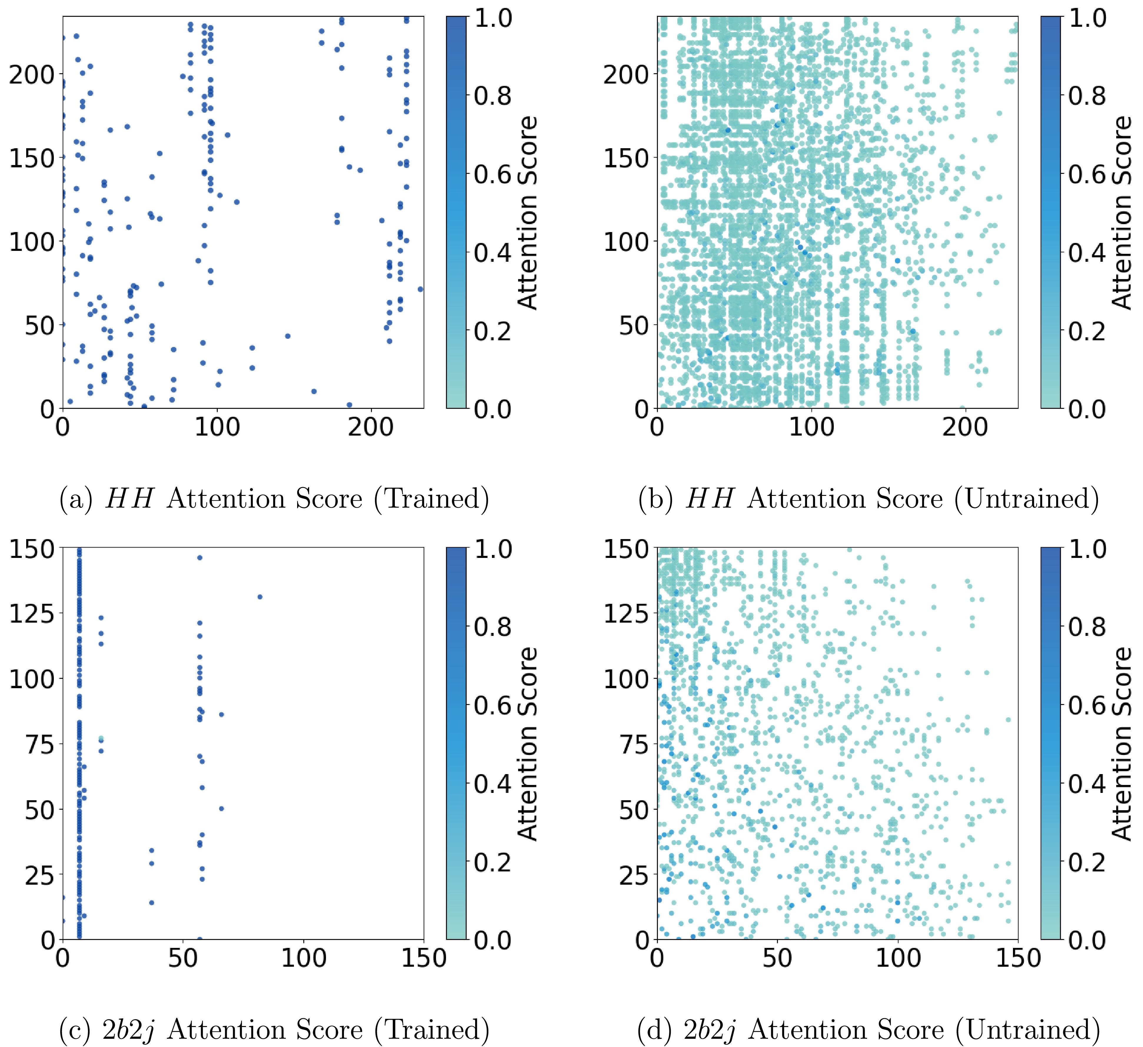

Figure 9.  (color online) The attention score (elements in attention matrix) for $ HH $ (upper panels) and $ 2b2j $ (lower panels) processes after (left panels) and before (right panels) training. Note that we have removed the attention score below 0.01 to make the plot clearer.

To incorporate the spatial position of particles, particle types, and the jets to which they belong during visualization, we further visualize the Particle Attention Graph, focusing on the final layer of the P-MHA module. Each particle is represented as a point in the η-ϕ plane, as shown in Fig. 10 and Fig. 11 for $ HH $ and $ 2b2j $ processes respectively. Different marker shapes are used to distinguish particle types: $ \times $ for mesons, $ \triangle $ for charged hadrons, $ \blacktriangledown $ for neutral hadrons, $ \bullet $ for photons, and $ + $ for electrons. Particles within the same jet, which is reconstructed using anti-$ k_t $ algorithm, are shown in the same color, while particles outside any jet are shown in gray. Note that this color information is just used for visualization. The opacity of each point is proportional to the transverse momentum $ p_T $ of the corresponding particle. The color of the connecting lines represents the attention score between particles. Solid lines indicate connections between particles inside jets, while dashed lines indicate connections involving out-of-jet particles. Note that to make the plot clear without full of low-weight connections, we only include the connections with weight higher than 0.5.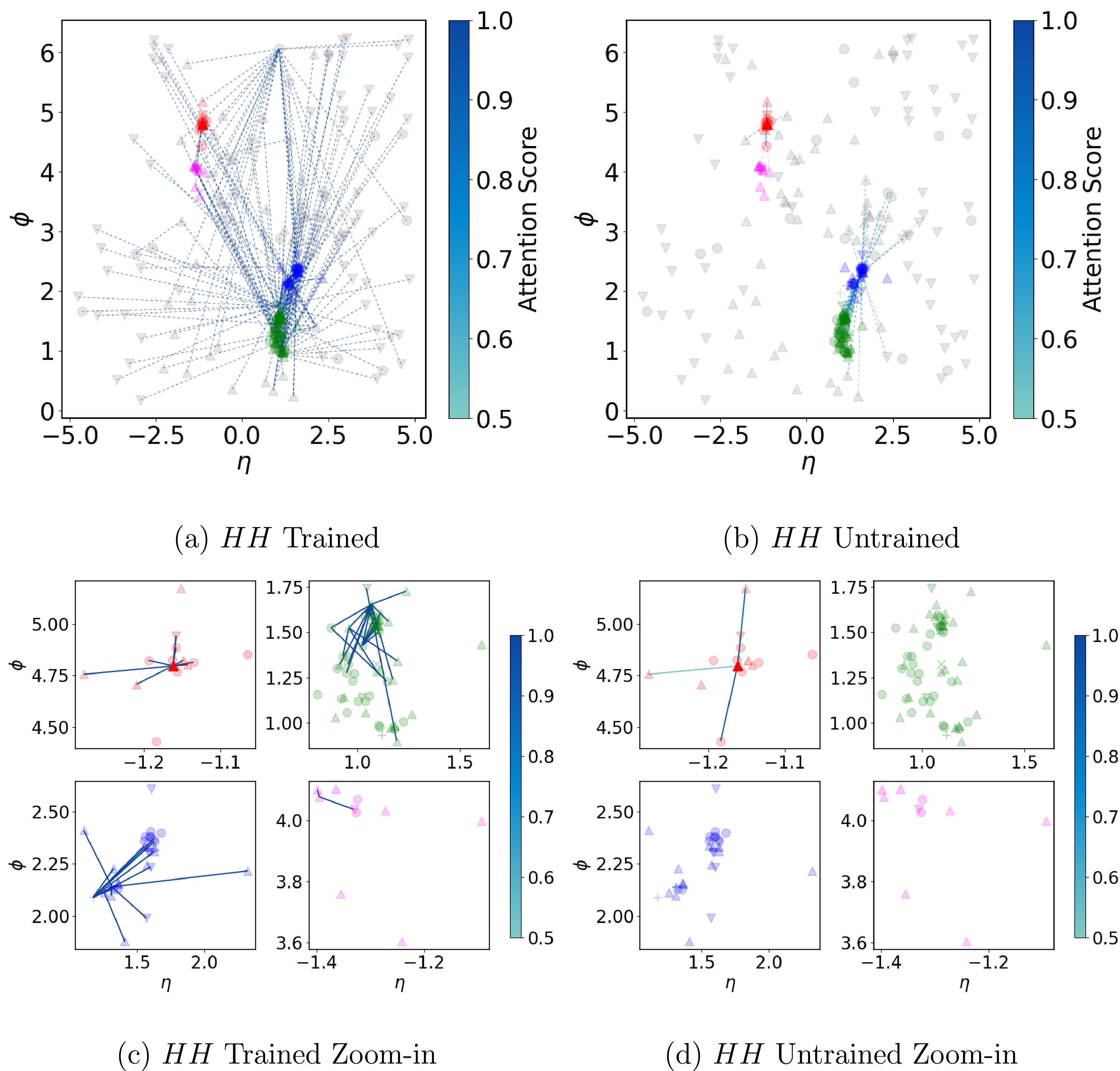

Figure 10.  (color online) Attention graphs for $ HH $ processes before and after model training. The lower panels show the connections within a single jet.

Figure 11.  (color online) Attention graphs for $ 2b2j $ processes before and after model training. The lower panels show the connections within a single jet.

In the upper panels of both Fig. 10 and Fig. 11, the connections in the whole η-ϕ plane are shown after (upper left) and before (upper right) the training for $ HH $ and $ 2b2j $ processes respectively. Similar to that in Fig. 9, the connections among particles become stronger after the training for both $ HH $ and $ 2b2j $ processes. To be more clear about the connections that are established during the training, for each process, we also provide the corresponding zoom-in view of the attention graph in the lower panels of Fig. 10 and Fig. 11. It is clear that the training also strengthen the connections within jets from the information about the whole event. By comparing these visualized attention graph, we conclude that the trained model is capable of focusing on the important particle pairs in an event and learning relationships within and between jets by training on the event-level instead of reconstructed objects. This capability underpins the model's outstanding performance and the possibility to the end-to-end event classification by event-level training. However in depth studies of what specific feature and relations have been learnt during the training is also very important to fully understand the underlying mechanism of the algorithm. This is a challenging task which we will leave for future works.

In this work, we employ a deep neural network architecture based on ParT to enhance the sensitivity of the Higgs self-coupling measurement through $ HH\to b\bar{b}b\bar{b} $ at the LHC which suffers from complex QCD backgrounds. With the help of the attention mechanism, the model can focus on important relationships among input features, enabling robust event classification when trained on full event-level information. The performance of such classifier is evaluated across 9 event categories achieving $ \text{AUC}\approx 0.9 $ for most categories, significantly distinguishing one process from the rest. In current study, we focus on $ HH\to b\bar{b}b\bar{b} $ analysis. However, it can actually be applied to other analysis with very minor modifications.

The studies in this work demonstrate the possibility of using the ParT model beyond the jet-tagging task. By treating the entire event as a single fat jet, the model achieves high classification accuracy while circumventing the error-prone explicit jet-pairing process inherent in traditional event reconstruction. Such approach streamlines analysis by directly utilizing the full event information and demonstrates the potential of such end-to-end analysis in collider phenomenology studies.

By applying the model to $ HH\to b\bar{b}b\bar{b} $ studies at the HL-LHC, the model constrains the Higgs self-coupling $ \kappa_\lambda $ to $ (-0.25,\,5.41) $ at 68% CL, which achieves around 44% improvement in precision compared with the traditional cut-based approach. The comparison against other ML methods further highlights the advantages of the Transformer-based architecture and the event-level analysis, particularly in capturing the correlations within high-dimensional event data. Further, the attention mechanism naturally provide the interpretability of the model which can also help us understanding what are the most important features and correlations when trying to separate different processes.

The authors gratefully acknowledge Huilin Qu, Congqiao Li, Sitian Qian and Kun Wang for their insightful discussion on the ParT, as well as Huifang Lv for her valuable contributions during the early stages of this project. The authors gratefully acknowledge the valuable discussions and insights provided by the members of the China Collaboration of Precision Testing and New Physics (CPTNP).