On the pole trajectory of the subthreshold negative parity nucleon with varying pion masses

A subthreshold pole with quantum number $ J^{PC} = 1/2^- $, named $ N^*(920) $, has been established in the $ S_{11} $ channel of $ \pi N $ scatterings. It has been firstly suggested in analyzing $ \pi N $ scattering data [1, 2] using the product representation for partial wave amplitudes (PWAs) [3−5], which comes from the correct treatment of the left hand cuts and unitarization [6, 7]. The pole is also confirmed using naive K-matrix approach [8] and $ N/D $ method [9]. Its existence is firmly established in a Roy-Steiner equation analysis in Ref. [10], with the pole location $ \sqrt{s} = (918 \pm 3)-i(163 \pm 9)\mathrm{MeV} $, and is reconfirmed in Ref. [11] at $ (913.9\pm1.6) -i(168.9\pm3.1)\mathrm{MeV} $. Its properties in turn naturally become a subject of research interest as much is left to be desired.

One might wonder why this state has a mass below the threshold but can still exhibit a large decay width to $ \pi N $. One could try to understand this problem from two perspectives. The first perspective involves recognizing that the usual concept of particle decay—where one particle decays into two or more particles—is defined only within the framework of perturbation theory. Strictly speaking, unstable particles cannot appear as in- and out-states of the S matrix; they can only be defined as poles on the second Riemann sheet of the analytically continued S matrix. These states exist solely as intermediate states in scattering processes. When a pole lies near the physical region, i.e. being a narrow resonance with a long lifetime, the imaginary part of the pole position approximately coincides with half of the decay width of the state calculated in perturbation theory. For poles far from the physical region, such as those associated with the σ and κ resonances, they can only be interpreted as intermediate states represented by poles of the S matrix. These states may induce moderate changes in phase shifts, which is why their existence has been a topic of extensive debate in the past. The second perspective is from the usual understanding that the invariant mass of an unstable intermediate state does not have a fixed value but instead exhibit a mass distribution. A state with a large width has a very broad invariant mass spectrum, with its central value roughly corresponding to the pole mass. This means that there is a greater probability for such a state to have an invariant mass far from this central value compared to narrow resonances. In the case of $ N^*(920) $, even though the central value of its mass distribution lies below the decay threshold, there remains some possibility for it to have an invariant mass above the threshold, allowing it to decay into $ \pi N $.

The early work on the properties of $ N^*(920) $ is its coupling to $ N\gamma $ and $ N \pi $ [12]. It is found that its coupling to $ N \pi $ is considerably larger than that of $ N^*(1535) $, while its coupling to $ N\gamma $ is comparable to that of $ N^*(1535) $. Here in this paper we will focus on the $ N^*(920) $ pole trajectory with varying pion masses.

In the literature, the σ pole trajectory with varying π masses has been a rather hot topic for discussions, see for example Refs. [13, 14] and references therein. Remarkably a model independent Roy equation analysis has been carried out to thoroughly solve the issue [15]. The study of the σ pole trajectory with varying $ m_\pi $ is important, since it opens a new window in exploring non-perturbative strong interaction physics provided by lattice QCD calculations. An alternative study based on $ O(N) $ linear σ model [16, 17] finds similar results comparing with that of Ref. [15], hence providing further evidence that the σ meson may be more reasonably described as “elementary”, in the sense that it is, the same as pions, described by an explicit field degree of freedom in the effective chiral lagrangian ¹. Inspired by this, we in this paper adopt the effective lagrangian with a linearly realized chiral symmetry. To be specific we use the renormalizable toy linear σ model with nucleon fields, though it is known that renormalizability condition is not at all a physical requirement when describing low energy hadron physics. In short, we use linear σ model rather than the χPT lagrangian, mainly for theoretical considerations ², though we believe the two give more or less the same results at qualitative level.

In the following we begin by a brief introduction of the linear σ model with nucleons in Sec. II, and calculate the σ pole trajectory using [1,1] Padé approximation in Sec. III. As it is verified that the unitarity approximation does give a similar σ pole trajectory as comparing with that of Ref. [15], it is satisfactory to use the same approximation method to further explore the $ N^*(920) $ trajectory, which will also be discussed in Sec. III. Sec. IV is devoted to discussions and conclusions.

The linear σ model [21] (LSM) lagrangian with a nucleon field can be written as follows:

where $ \Psi_0 $ is the isospin doublet denoting bare nucleon fields, and $ {\boldsymbol{\pi}}_0,\sigma_0,\mu_0, g_0, \lambda_0 $ are bare π meson triplet, σ field, a mass parameter, and couplings, respectively. The renormalized quantities are related to bare ones through:

Spontaneous chiral symmetry breaking (χSB) occurs when the σ vacuum expectation value (vev) $ \langle \sigma \rangle = v \neq 0 $, generating three zero-mass Goldstone bosons: $ \pi^i,\quad i = 1,2,3 $ in the absence of explicit χSB term $ C\sigma_0 $. To perform a perturbative calculation, one shifts $ \sigma\to\sigma + v $ such that $ \langle \sigma \rangle = 0 $ and gets,

with

and the renormalization constants are defined as

From Eq. (4) we obtain the relation between $ m_\pi $ and $ m_\sigma $:

This relation holds if the renormalization constant $ Z_\lambda $ is chosen as

The other renormalization constants are determined by the following conditions, as done in Ref. [22]:

● To determine $ \delta m_\pi^2 $ and $ Z_\phi $, we demand that the full π propagator $ \Delta_\pi(s) $ satisfies

● $ \delta m_\sigma^2 $ can be determined by requiring the real part of the inverse σ propagator, $ i \Delta^{-1}_{\sigma}(s) $, to vanish when $ s\to m_\sigma^2 $, i.e.,

Notice that the parameter $ m_\sigma $ can not be identified as the σ pole mass when $ m_\sigma>2m_\pi $ since $ i \Delta_\sigma^{-1}(m_\sigma^2) $ is complex in this situation. On the other hand, if $ m_\pi $ increases to be large enough such that $ m_\sigma < 2m_\pi $, then $ i \Delta_\sigma^{-1}(m_\sigma^2) $ becomes real and $ m_\sigma $ is just the pole mass.

● $ Z_\psi $ and $ Z_g $ are determined by forcing the full nucleon propagator $ \Delta_N(\not{p}) $ behaving like:

The results for the renormalization constants and counter terms under these renormalization conditions are listed in Appendix A.

In LSM, there are four free parameters and they can be chosen as λ, $ m_\sigma $, $ m_\pi $, g. From Eqs. (6) and (4), the vev v and the nucleon mass $ m_N $ are expressed by:

In the physical situation, $ m_\pi = 0.138\mathrm{GeV}, m_N = 0.938\mathrm{GeV} $, and v is identical to the pion decay constant $ f_\pi $ at tree level, whose experimental value is $ 0.093 \mathrm{GeV} $ so that $ g\simeq 10 $. From PCAC, one also obtains $ C\sqrt{Z_\phi} = f_\pi m_\pi^2 $, and the pion decay constant $ f_\pi $ are related to v by [23]:

At the one-loop level, this equation reads:

Numerical tests reveal that the left hand side of this equation has a negligible effect within the parameter regime used in our following calculations [22]. Therefore, $ f_\pi $ is still approximately equal to the vev v at the one-loop level ³.

Since our purpose of using the LSM is to approximate QCD which has only two free parameters, i.e., gauge coupling or $ \Lambda_{QCD} $ and the quark mass, whereas LSM has four — $ (g,m_N,m_\sigma,m_\pi) $, this leaves some room for manipulation of $ m_\pi $ dependence of parameters. In principle, only two parameters are independent for LSM to serve as a low-energy effective field theory of QCD. Since we are considering the $ m_\pi $ dependence, we can choose $ m_\pi $ as one independent parameter and select another parameter to be independent of $ m_\pi $, leaving the other two parameters dependent on $ m_\pi $. Given the fact that χPT encodes the correct $ m_\pi $ dependence from QCD, it can be used to provide the missing $ m_\pi $ dependence in LSM. Since $ f_\pi $ appears in both theory, we make use of χPT results to fix the dependence of $ f_\pi $ on $ m_\pi $ ⁴, which has been calculated up to NNLO in Refs. [24, 25]. Rewriting in terms of F and $ m_\pi $, $ f_\pi $ is expressed as [24, 25]

where these low energy constants (LECs) are obtained in Ref. [26] by a full analysis on lattice data. In the following calculations, we impose this condition to constrain the $ m_\pi $ dependence of v by using Eq. (12). Another constraint from χPT is the $ m_\pi $ dependence of $ m_N $. We require the dependence of $ m_N $ on $ m_\pi $ to match the $ {\cal{O}}(p^5) $ result of baryon χPT [27]. From the second equation in (11), the $ m_\pi $ dependence of g is also fixed. With one remaining free parameter, from the first equation in (11), we consider two alternative simple assumptions to proceed: to fix $ m_\sigma $ such that λ is dependent on $ m_\pi $ or vice versa. Since these two choices produce similar qualitative results, we choose the first one in discussing the $ \pi\pi $ scatterings and only provide the results in $ \pi N $ scatterings for both choices.

This section is devoted to the study of the σ pole and the $ N^*(920) $ pole dependence on varying pion masses. This analysis is meaningful in understanding the non-perturbative aspects of low energy strong interaction physics, especially in the era when lattice QCD studies become more and more prosperous ⁵. For the former, the σ pole trajectory is well understood [15, 29] while knowledge of $ N^*(920) $ trajectory is absent yet, from either lattice QCD or analytical studies.

We will study the two trajectories based on the renormalizable linear σ model with nucleons. The reason why we choose such a model is already discussed in the introduction. We in the following firstly re-analyze the σ pole trajectory using [1,1] Padé approximation ⁶. It will be found that the trajectory obtained is in rather good agreement with that of Roy equation analyses and $ O(N) $ model results qualitatively. This is because, unlike the unitarization using χPT amplitude, the t and u-channel σ exchange is taken into account here, which is the requirement of crossing symmetry.

Basically there can be two ways to extract the σ pole location: one is from the σ propagator, another is from the unitarized $ \pi\pi $ scattering amplitude. They are not equivalent under the approximations being used, however. The propagator is obtained by using a Dyson resummation of self energy bubble chain, and is essentially a one loop calculation, whereas the pole in the unitarized amplitude contains more complete dynamical input ⁷. Therefore we adopt the scattering amplitude to extract the pole locations.

The $ \pi\pi $ elastic scattering amplitude is written as:

where $ \alpha,\beta,\gamma $ and δ are isospin indexes and $ s,t $ and u are Mandelstam variables subject to the constraints $ s+u+t = 4m_\pi^2 $. $ A(s,t,u),B(s,t,u) $ and $ C(s,t,u) $ are Lorentz invariant amplitudes. The total isospin $ I = 0 $ amplitude $ T^0(s,t,u) $ can be derived as

Partial wave amplitude(PWA) is defined as

where $ P_J $ is the Legendre polynomial. The elastic unitarity reads:

with

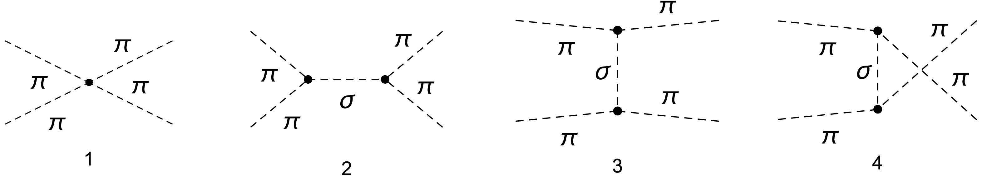
The PWA has been calculated up to one-loop level within LSM neglecting nucleon contributions. At tree level, the Feynman diagrams contributing to $ \pi\pi $ scattering amplitudes are presented in Fig. 1.

Figure 1.  The tree-level Feynman diagrams contributing to ππ scatterings.

The corresponding invariant amplitude $ A(s,t,u) $ reads:

The invariant amplitudes $ B(s,t,u) $ and $ C(s,t,u) $ are related to $ A(s,t,u) $ via crossing symmetry:

From perturbative unitarity in LSM we have:

where $ T^{0}_{0t}(s) $ and $ T^{0}_{0l}(s) $ denote the tree-level and the one-loop PWAs, respectively. Combining Eq. (16)-(17), the tree-level PWA is obtained:

At one-loop order, it is tedious to present all Feynman diagrams and their corresponding results, which exceed 50 diagrams [31]. Therefore, we will not include those amplitudes in this paper ⁸. With Eq. (22), it is easy to prove that the $ [1,1] $ Padé approximant

satisfies elastic unitarity.

The σ resonance corresponds to the pole of the PWA on the second Riemann sheet (RSII) of complex s plane, or the zero of partial wave S matrix:

on the first Riemann sheet (RSI).

According to Eq. (24), the numerator of $ T^{0[1,1]}_{0}(s) $, i.e., $ T^0_{0t} $, contains a first-order pole at $ m_\sigma^2 $. When $ m_\sigma>2m_\pi $, in the denominator $ 1-T^{0}_{0l}/T^0_{0t} $, there also exists a first-order pole because the loop-level amplitude $ T^0_{0l}(s) $ contains a second-order pole at $ m_\sigma^2 $ from the one-loop σ propagator as shown in the right diagram of Fig. 2. This causes $ T^{0[1,1]}_{0}(s) $ to be finite at $ m_\sigma^2 $. Thus, in this situation $ m_\sigma $ is not the pole mass of σ and the σ pole position would lie on the second Riemann sheet. On the contrary, with $ m_\pi $ growing up to $ 2m_\pi>m_\sigma $, the second-order pole in $ T^0_{0l}(s) $ transforms to a first-order pole because the residue being proportional to $ \Sigma(m_\sigma^2) $ equals zero due to the renormalization condition (8). In this case, the denominator of Eq. (24) is finite at $ m_\sigma^2 $, and the numerator remains a pole at $ m_\sigma^2 $ which corresponds to the σ bound state.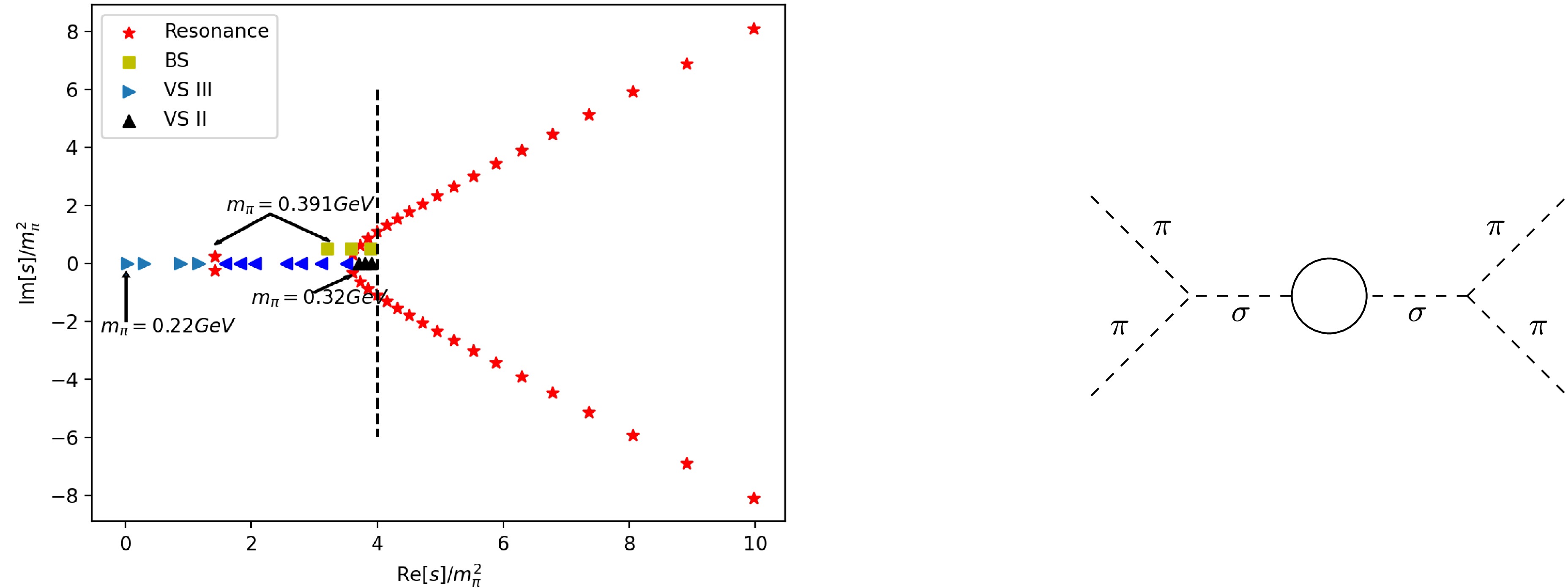

Figure 2.  (color online) The trajectory of σ resonance with $ m_\pi$ variation. The vertical dashed line denotes the physical threshold. Right: the contribution of σ self-energy correction to $ \pi \pi$ amplitude.

To obtain the specific trajectories through numerical calculation, we choose a suitable $ m_\sigma = 0.7\mathrm{GeV} $ such that σ pole locates at about $ (0.47-i0.16) $ GeV at physical pion mass. ⁹ Then, fixing this $ m_\sigma $ parameter and taking into account the relation between $ f_\pi $ and $ m_\pi $, the trajectory of σ pole with increasing $ m_\pi $ is depicted in Fig. 2. The σ resonance falls down to real axis below the threshold from the complex plane above the threshold, becoming two virtual states (VSI and VSII) when $ m_\pi $ increases from physical value to $ m_\pi\simeq 0.32\mathrm{GeV} $. One of them (VSII) runs towards threshold and finally crosses the threshold to the real axis below the threshold on RSI, turning into a bound state when $ 2m_\pi > m_\sigma $. On the other hand, the other virtual state (VSI) runs away from the threshold and collides with the third virtual state (VSIII) which appears from the left-hand cut when $ m_\pi\simeq 0.22\mathrm{GeV} $. Then these two virtual-state poles turn into a pair of resonance poles on the complex plane. The trajectory is similar to that of the Roy equation [15] and the $ N/D $ modified $ O(N) $ model [16], but now the critical point ($ m_\sigma/2 $) when σ becomes a bound state can be determined analytically from the expression of Padé amplitude. Note that appearance of VSIII is a result of the σ exchange in the crossed channels which is the requirement of crossing symmetry. However, this effect is not taken into account in the unitarized χPT calculations and thus there is no such a virtual state found there [13].

Having examined that the σ pole trajectory can be satisfactorily reproduced in the scheme of linear σ model with Padé unitarization, we are confident to step forward by studying the $ N^*(920) $ pole trajectory in the linear σ model with nucleon field, in the next subsection.

For the process $ \pi^a(p)+N_i(q)\to \pi^{a^\prime}(p^\prime)+N_f(q^\prime) $, the isospin amplitude can be decomposed as:

where $ \tau^a $ ($ a = 1,2,3 $) are Pauli matrices, and $ \chi_i $ ($ \chi_f $) corresponds to the isospin wave function of the initial (final) nucleon state. The amplitudes with isospins $ I = 1/2, 3/2 $ can be written as

Taking into account of the Lorentz structure, for an isospin indices $ I = 1/2,3/2 $, the amplitude can be represented as

with the superscripts $ (s), (s^\prime) $ denoting the spins of Dirac spinors and three Mandelstam variables $ s = (p+q)^2, t = (p-p^\prime)^2, u = (p-q^\prime)^2 $ obeying the constraint $ s+t+u = 2m_N^2+2m_\pi^2 $. The channel with orbit angular momentum L, total angular momentum J and total isospin I denoted as $ T(L_{2I2J}) $ is defined as:

where the definition of partial wave helicity amplitudes are written as:

with

$ z_s = \cos\theta $ with θ the scattering angle in center of mass frame (CM). The PWAs $ T^{I,J}_{\pm} $ satisfy unitarity condition:

The full tree-level amplitudes of $ \pi N $ scatterings in LSM are given by three diagrams as depicted in Fig. 3.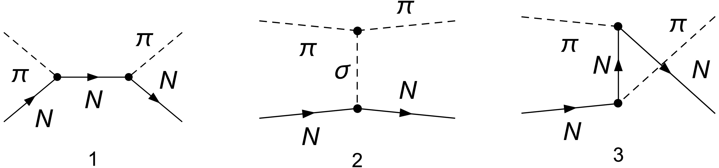

Figure 3.  The tree-level Feynman diagrams contributing to πN scatterings.

Contributions to invariant amplitudes $ A^{1/2}(s,t,u) $ and $ B^{1/2}(s,t,u) $ at tree level read

According to Eq. (31), after partial-wave projection, the expressions of $ A^{1/2,1/2}_{C/S} $ and $ B^{1/2,1/2}_{C/S} $ are listed as follows,

with $ k = \sqrt{s}\rho(s,m_\pi,m_N)/2 $ being the magnitude of 3-momentum in CM and

$ B_C(s) $ and $ B_S(s) $ contain the u-cut in the interval $ (c_L = (m_N^2-m_\pi^2)^2/m_N^2,c_R = m_N^2+2m_\pi^2) $ from the logarithmic term generated by u-channel nucleon exchange, as depicted in the 3rd diagram in Fig. 3. When $ 2m_\pi < m_\sigma < 2m_N $, the $ I(s) $ function contains circular arc cuts [8] centered at the origin with a radius of $ m_N^2-m_\pi^2 $. At one loop, the circular cut emerges due to continuous two-particle spectrum, which covers the circular arc cut.

After partial-wave projection, the perturbative PWAs will be unitarized by $ N/D $ method ¹⁰, which boils down to solving an integral equation about $ N(s) $ function:

The subtraction point $ s_0 $ and subtraction value $ N(s_0) $ can be chosen appropriately and $ U(s) $ function should be analytic when $ s>s_R $, such that $ N(s) $ only contains left hand cuts

where the subscript L denotes the left-hand cut where the integration is performed. The discontinuity of the amplitude $ M(s) $ need to be an input from the perturbative calculation. Since the dispersion relation of the amplitude on the left-hand cut essentially gives the amplitude with the right-hand cut integral subtracted up to a polynomial, we can use the perturbative amplitude with the right-hand cut dispersion integral subtracted to estimate $ U(s)-U(s') $ directly in the following.

The amplitude satisfying the unitarity condition can be constructed as (we use $ M(s) $ to represent $ \pi N $ scattering amplitude in $ S_{11} $ channel):

One can numerically solve the equation by inverse matrix method, after introducing a cutoff Λ such that the integral interval becomes $ (s_R,\Lambda) $ instead of $ (s_R,\infty) $. In the following, $ s_0 $ and Λ, are fixed at the $ \pi N $ threshold $ s_R $, and the nearest inelastic threshold $ (m_N+m_\sigma)^2 $ in perturbation theory, respectively. Since the once-subtracted dispersion relation is used, the integrand above this cut off is highly suppressed and the final results would be roughly independent of this cut off choice.

At tree level, since there is already no right-hand cut in tree-level amplitude $ M_t $, we set $ U(s) $ equal to $ M_t(s) $, and $ N(s_0) $ equal to $ M_t(s_0) $ which fixes $ M(s_0) = M_t(s_0) $. Starting from $ m_\sigma $ at $ 0.55\mathrm{GeV} $ ¹¹, we have performed two sets of calculations: one with fixed $ m_\sigma $ and the other with fixed λ as $ m_\pi $ increases. A pole at $ (0.94 - 0.14i)\mathrm{GeV} $ corresponding to $ N^*(920) $ can be found on the second sheet with physical pion and nucleon mass. The pole trajectories on RSII with $ m_\pi $ increasing for both cases are shown in Fig. 4 with $ \text{Im}W>0 $ ($ W\equiv\sqrt{s} $) points.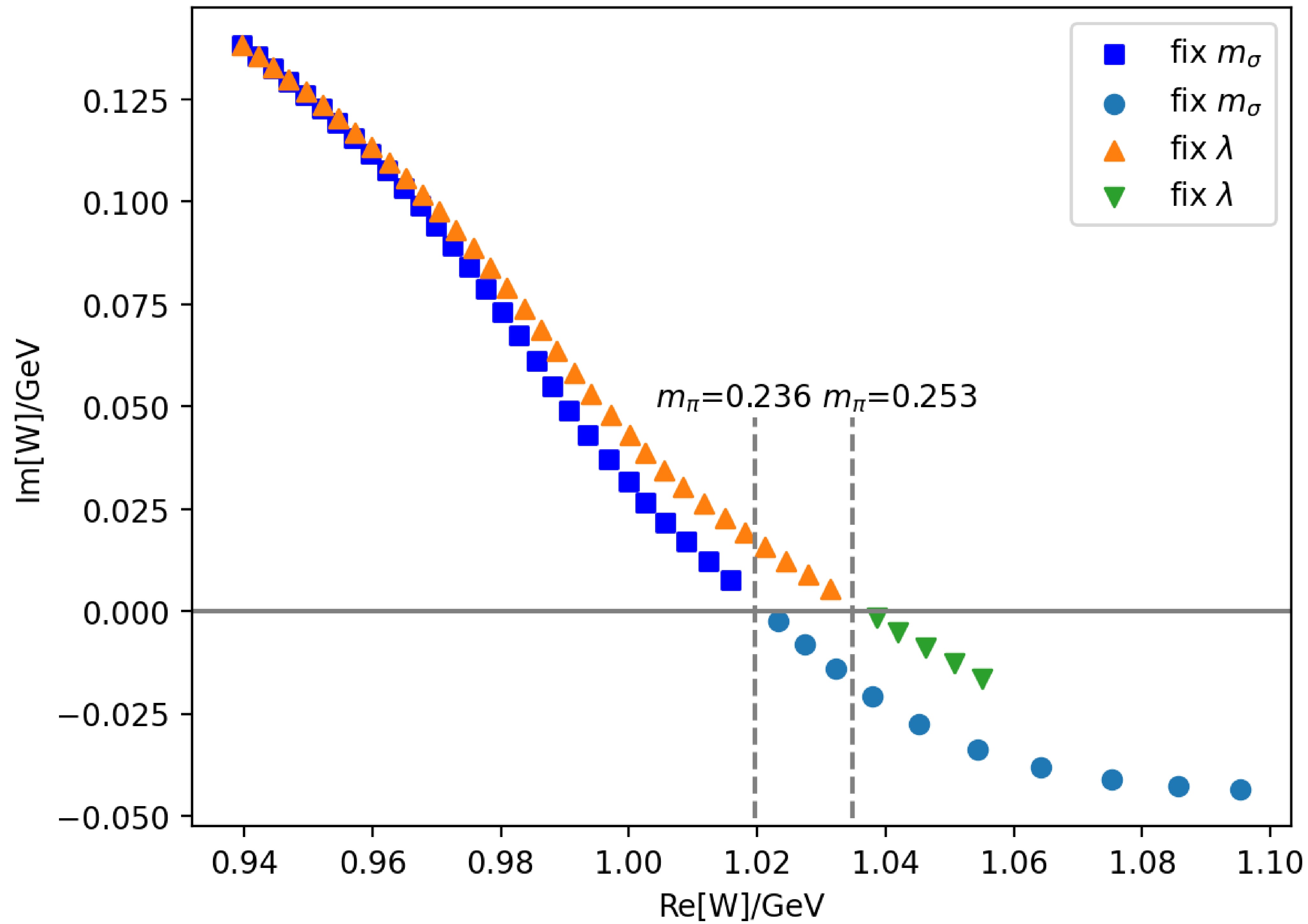

Figure 4.  (color online) The trajectories of $N^*(920)$ as $m_\pi$ ranges from the physical value to $0.27\mathrm{GeV}$ for both cases of fixed $m_\sigma$ and fixed λ at tree level. The points with $\text{Im}[W]>0$ are the zeros (RSI) of S matrix for different pion masses and those with $\text{Im}[W]<0$ are the zeros of the $S_+$ function (see the text). The vertical dashed lines correspond to roots obtained by solving equation (43) for $m_\pi = 0.236\mathrm{GeV}$ and $0.253\mathrm{GeV}$, respectively. We also tested the cases with cut offs at $2{\rm{GeV}}^2$ and $3 {\rm{GeV}}^2$ respectively and found no distinguishable differences in the results.

The imaginary part of $ N^* $ pole position decreases while the real part grows when $ m_\pi $ increases in both cases, causing the poles to move toward the u-cut bounded by two branch points at $ c_R $ and $ c_L $. Since the two conjugate $ N^* $ poles on RSII correspond to zeros of the S matrix on RSI, we consider the zero points in the following. After the zeros reach the u-cut, in principle there could be two possibilities: (1) the zeros move away from each other on the real axis after collision; (2) the zeros cross the u-cut and enter adjacent sheets defined by the logarithmic branch of the u-cut. However, we will show that the first senario is impossible for $ \pi N $ scattering.

In the first senario, if the $ N^* $ zeros reach the u-cut at $ s_* \in(c_L,c_R) $ at critical pion mass $ \tilde{m}_\pi $ and then separate to two virtual state zeros, this implies that $ s_* $ must be a second-order zero of the S matrix. A necessary condition is that $ s_* $ is also a second-order zero of the imaginary part of S matrix, i.e., $ \text{Im}[S(s_*)] = 0 $ and $ \text{Im}[S'(s_*)] = 0 $. The first condition gives

as $ 2i\rho(s_*,m_\pi,m_N) $ is real on the u-cut. Since the sole contribution to the imaginary part of PWA arises from the u-channel nucleon pole $ \dfrac {g}{u-m^2_N} $ in the partial wave projection, which is non-perturbative and remains valid to all orders of perturbative expansions ¹², the zero of the imaginary part of PWA on the u-cut in general case always coincides with tree level $ \mathrm {Im}M_t(s) $. According to the expression of $ M_t(s) $, the condition $ \text{Im} M_t(s) = 0 $ on the u-cut is equivalent to

This equation has only one solution at $ W_*\simeq m_N-\dfrac{m_\pi^4}{4m_N^3} $ inside u-cut.

Similarly, $ \text{Im}[S'(s_*)] = 0 $ requires that the derivative of the left-hand side of Eq. (43) vanishes at the same point. However, this is impossible: differentiating the left-hand side of Eq. (43) yields $ m_N (m_N - 3 W) (m_N + W) $ (only consider the term in brackets), whose only reasonable root $ W^\prime_* = m_N/3 $ does not satisfy Eq. (43). Therefore, the nonexistence of a second-order zero and only one zero in imaginary part of PWA excludes the first scenario.

In the context of the $ N/D $ method, the zero point of the S matrix at $ s_* $ requires

Since $ D(s) $ function is real on the left-hand cuts, the requirement $ \text{Im} S = 0 $ leads to

where we have used the fact that $ 2i\rho(s_*,m_\pi,m_N) $ is real. Thus, the necessary condition for the S matrix to vanish at $ s_* $ is $ \text{Im} M_t(s_*) = 0 $ which is reduced to (43). Note that the property that the zero of the imaginary part of S matrix on the u-cut coincides with that of Im$ M_t(s) $ is not only preserved in $ N/D $ method but also respected by Padé or K-matrix unitarizations. A proof is provided in App. B.

It is, however, worth mentioning that the first scenario we have just excluded is actually what was happening in the case of $ \pi\pi $ scatterings (see Fig. 5).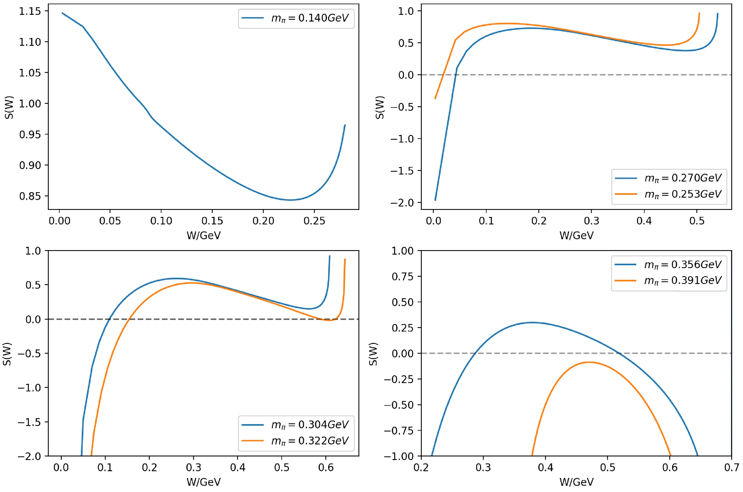

Figure 5.  (color online) The S matrix values for $\pi\pi$ scatterings between the left hand cut and the threshold using the results of the previous section. Initially, no S-matrix zeros exist in this region (upper-left subfigure). As $m_\pi$ increases, a virtual-state zero (VSIII) emerges from the left-hand cut (upper-right). The sigma resonance turns into virtual-state zeros when the S matrix's local minimum contacts the real axis, generating a second-order zero precisely at this point. Subsequently, the two virtual-state zeros (VSI and VSII) split apart along the real axis (lower-left). VSI later becomes a bound-state pole of the S-matrix, leaving two virtual-state zeros (VSII and VSIII). These two zeros then coalesce on the real axis and move into the complex plane as resonance zeros (lower-right).

Having excluded Case 1, the only possibility is that the $ N^* $ zeros cross the u-cut and enter adjacent Riemann sheets defined by the u-cut. To trace the zeros further, the S matrix must be analytically continued onto these sheets. The analytically continued S matrix from the upper (lower) half-plane to the adjacent lower (upper) half-plane, $ S_+ $ ($ S_- $), can be obtained by adding $ \pm 2\pi i $ to the logarithmic function $ \ln(\dfrac{s(s-c_R)}{m_N^2(s-c_L)}) $ in the unitarized S matrix on RSI. Therefore, after $ N^* $ crosses the u-cut, we should find the zero of $ S_+ $ on the adjacent lower half-plane or the zero of $ S_- $ on the upper adjacent half-plane to continuously trace the trajectories. Fig. 4 shows how the zeros approach the u-cut, cross it at the critical point (marked by vertical dashed lines in Fig. 4) where $ \text{Im}[S] $ vanishes, and subsequently become the zeros of $ S_+ $ as $ m_\pi $ increase for both schemes: fixed $ m_\sigma $ and fixed λ.

Notably, tracing the poles across the u-cut starting from RSII is consistent with tracing the zeros starting from RSI. The $ S^{II} $ (S matrix on the RSII) is defined

Modifying the logarithmic function $ \ln\left(\dfrac{s(s-c_R)}{m_N^2(s-c_L)}\right) $ in $ S^{II}(s) $ similarly results in

Therefore, the zeros of $ S_\pm $ correspond to the poles of $ S^{II}_{\pm} $.

In above, we have actually established a mathematical theorem: if the zero reaches the u-cut, it must meet the cut at $ W = W_* $ defined by Eq. (43), and will cross onto the adjacent sheet. Nevertheless, this theorem does not tell why the pole should move toward the real axis. Then the next question becomes whether the zero will ever approach the u-cut and why. At tree level, the $ N^* $ resonance does reach the u-cut. However, there may still exist other possibilities for the $ N^* $ pole of the full amplitude: it could move onto the real axis within the interval $ (c_R,s_R) $ outside the u-cut, or it may even never touch the real axis. To further explore these possibilities, we extend the calculations to one-loop level in the following.

At one-loop level, parameter $ N(s_0) $ is set equal to $ M_t(s_0)+M_l(s_0) $ and $ U(s) $ is written as:

with $ M_l(s) $ the one-loop correction to the PWA. The full one-loop amplitude has been known for a long time [32], and after partial wave projection, the PWA is too long to be presented here ¹³. The third term in the above expression ensures $ U(s) $ to be analytic in the interval $ (s_R,(m_N+m_\sigma)^2) $ and consistent with perturbative unitarity:

The nearest inelastic cut in the one-loop amplitude is above $ (m_\sigma+m_N)^2 $ in real axis, and thus we fix the cutoff $ \Lambda = (m_N+m_\sigma)^2 $ such that the unitarized amplitude satisfies the single channel unitary condition in the interval $ (s_R,(m_N+m_\sigma)^2) $.

A pole at $ (0.92 - 0.15i)\mathrm{GeV} $ corresponding to $ N^*(920) $ can be found on the second sheet with physical pion and nucleon masses. The pole trajectories of $ N^*(920) $ for the tree level and the one-loop level as $ m_\pi $ increases are shown in Fig. 6. At one-loop level, the trend of $ N^*(920) $ trajectories is similar to that at tree level: both move toward the real axis in the beginning. However, when $ m_\pi $ gets larger, the difference emerges. The one-loop zero does not seem likely to fall onto the real axis at least up to $ m_\pi = 0.36\mathrm{GeV} $. We do not further test larger $ m_\pi $ since chiral expansions, which constrains the $ m_\pi $ dependence of $ m_N $ and $ f_\pi $ in our calculations, may become more and more inaccurate at larger $ m_\pi $.

Figure 6.  (color online) Up: The dot points and triangle points denote the trajectories of $N^*(920)$ with $m_\pi$ variation from $0.138\mathrm{GeV}$ to $0.360\mathrm{GeV}$, at one-loop level and tree level for fixed λ, respectively. Down: the values of S matrix at one-loop level in intervals $(s_L, c_L)$ and $(c_R,s_R)$ on the first Riemann sheet. The red solid lines in the middle of the dashed lines denote the u-cuts.

We also studied the behavior of the two virtual states [33] lying in the interval $ ( s_L = (m_N-m_\pi)^2,c_L) $ and $ (c_R,s_R) $, respectively. The values of S matrix calculated with one-loop level input in the two intervals on the first Riemann sheet are plotted in Fig. 6, which demonstrates the fact that the S matrix equals to unity at $ s_L $ and $ s_R $ by definition while it tends to negative infinity when s is close to the two branch points $ c_L $ and $ c_R $. As a result, a zero point inside each interval occurs. The calculation reveals that the virtual states move toward $ s_R $ or $ s_L $ with increasing $ m_\pi $.

In this paper we have studied the σ pole trajectory and the $ N^*(920) $ pole trajectory with varying $ m_\pi $, in a linear σ model with nucleons, aided by certain unitarization approximations. The $ m_\pi $ dependence of $ f_\pi $ and $ m_N $ from the χPT are also taken into account, which renders the LSM more reasonable in approximating the low energy QCD. The σ pole trajectory is found to be in agreement with previous studies [15, 16]. The result on $ N^*(920) $ pole trajectory is novel. At tree level, the $ N^*(920) $ pole is found to move towards the u-cut on the real axis on the second Riemann sheet with increasing $ m_\pi $, ultimately crossing the u-cut and entering the adjacent Riemann sheet defined by the u-cut. At one-loop level, however, the $ N^*(920) $ still stays on the complex-plane at $ m_\pi = 0.36\mathrm{GeV} $ and even higher values. The intricate analytical structure of $ \pi N $ PWAs, including the circular cut and u-cut, which stems from the the dynamical complexity of $ \pi N $ interactions, increase the difficulty for predictions on the final fate of $ N^* $. The results presented in this paper can be useful in comparison with future lattice studies on $ \pi N $ scatterings. The next interesting topic for future studies would be to investigate the $ N^*(920) $ pole trajectory in the presence of temperature and chemical potential, and the old concept of parity doublet model may return with some new ingredients.

The counter terms and renormalization constants take following forms up to one-loop level,

The definitions of 1-point function $ A_0(m^2) $ and 2-point function $ B_0(p^2,m_1^2,m_2^2) $ are expressed as

$ B_0^\prime $ denotes the derivation with respect to the first argument.

In [1,1] Padé approximant, the ampltiude $ M(s) $

The fact that $ \mathrm{Im}[M_l(s)] = \mathrm{Im} [M_t(s)] $ on the u-cut causes the zero of Im$ M(s) $ to be the same as that of Im$ M_t(s) $ on the cut. As to the K-matrix, the amplitude is given by ¹⁴

Then, the Im$ S(s) $ on the u-cut reads:

Again, we get the same conclusion.