Application of physics-informed neural network on multidimensional quantum tunneling

Quantum tunneling is a fundamental phenomenon in quantum mechanics, where particles exhibit a finite probability of traversing potential barriers that exceed their kinetic energy [1]. First introduced in the context of alpha decay by Gamow [2], tunneling has evolved into a cornerstone concept with profound implications across various domains of physics and chemistry. In nuclear physics, tunneling is the main process of nuclear reaction phenomena such as fusion and fission, where particles overcome potential barriers at sub-barrier energies [3]. The study of tunneling between two nuclei offers valuable insights into phenomena related to power generation, astrophysical evolution, and the synthesis of superheavy elements. However, accurately modeling the tunneling process remains challenging due to the complexity of nuclear reactions, which involve multidimensional quantum tunneling by coupling the radial motion to the nuclear collective vibrations, single-particle excitations, transfer couplings, and so on.

The Numerov method is a widely used finite difference approach for theoretically describing tunneling processes involving real or imaginary nuclear potentials. Different modified versions of this method have employed to solve the multidimensional coupled-channels equations in programs such as CCFULL, CCqel and Fresco [4, 5]. The coupled matrix is typically constructed by accounting for the collective vibrations and/or rotations of the projectile and target. However, this method is known to exhibit numerical instabilities in the classically forbidden energy region, where wave functions can differ by orders of magnitude, leading to a loss of linear independence [6].

In addition to the usually used Numerov method, other sophisticated and high-accuracy numerical methods have been developed recently, including the Lagrange-mesh improved Numerov algorithm used in breakup reactions [7, 8], advanced complex scaling method [9, 10], the R-matrix method (RM) and the finite element method (FEM). The complex scaling method adopts a single set of reduced bases, allowing for efficient and simultaneous emulation across multiple channels and potential parameters of direct reactions. The RM solves the coupled-channels equations using Lagrange basis functions and the propagation method, which are capable of handling elastic scattering, breakup reactions, and transfer reactions of light nuclei [11−14]. This approach allows for straightforward calculations of matrix elements. Additionally, the propagation method is employed to save computation time when there is only local potential.

The FEM is recognized for its superior numerical accuracy compared to the Numerov method [15−17]. An efficient finite element program, KANTBP, has been developed to calculate the reflection and transmission matrices, and corresponding wave functions by solving coupled Schrödinger equations. Leveraging the program's high accuracy and careful consideration of non-diagonal matrix elements, it has successfully reproduced astrophysically significant deep sub-barrier fusion cross sections and their experimental S-factors [18−21]. Recently, an algorithm has been devised to solve the scattering problem in complex potential and single channel approximation, facilitating more accurate barrier distribution analyses of quasi-elastic reactions [22].

The aforementioned numerical techniques discretize the spatial domain and approximate Schrödinger equations, enabling the computation of wave functions and energy levels. However, in multidimensional quantum tunneling, effectively incorporating single-particle excitation and transfer coupling remains challenging. One of the core difficulty lies in the inherently high-dimensional nature of these problems, which leads to the curse of dimensionality [23, 24]. This underscores the urgent need for the development of novel solution methods. Deep learning, a subset of machine learning, exhibits enhanced capabilities in representing and simulating complex functions through its multi-hidden-layer architecture, making it particularly suitable for addressing high-dimensional problems.

In recent years, machine learning techniques, particularly deep neural networks, have emerged as promising tools for the solving partial differential equations (PDEs), with profound implications in physics, mathematics, and related fields [25−27]. Physics-Informed Neural Networks (PINNs) [28] represent a framework by integrating physical laws directly into the neural network's loss function. By encoding PDEs, initial conditions, and boundary conditions into the training process, PINNs enable the network to learn solutions that inherently satisfy the governing equations [29]. This approach has demonstrated promising applications in various fields, including fluid mechanics [30], characterization of internal structures and defects in materials [31], molecular dynamics and so on [32]. Recently, PINNs have been directly applied to solve the Schrödinger equation under harmonic oscillator and Woods-Saxon potentials, yielding ground state wave functions and energy levels [33]. Additional developments include Pauli Net [34] and Feynman Net [35], which employ deep learning approaches to solve multi-electron stationary Schrödinger equations, and also Feynman Net specifically addressing isospin-dependent nuclear many-body equations [36].

Despite these advancements, the application of PINNs to quantum scattering problems, particularly multidimensional quantum tunneling, remains relatively unexplored. This work aims to address this gap. The structure of the paper is as follows: Section II provides a detailed theoretical framework, including the formulation of the multidimensional Schrödinger equation and the implementation details of PINNs. Section III presents results for both the Eckart and Gaussian potentials, including comparisons with analytical solutions and FEM results. Finally, Section IV concludes the paper by summarizing the results and discussing the potential future directions.

Quantum tunneling is governed by the Schrödinger equation. For one-dimensional systems, the tunneling probability can be calculated analytically only for a limited number of potentials. For most realistic one-dimensional and higher-dimensional channels, numerical methods are required. In a multidimensional tunneling problem, for each channel n, the coupled-channel (CC) equation is expressed as:

where $ \phi_n(r) $ represents the radial wavefunction, r is the radial distance, N is the total number of coupled channels, $ \hbar $ is the reduced Planck's constant, and μ is the reduced mass of the system. The term $ W_{nm}(r) $ denotes the coupling potential between channels n and m, and E is the incident energy of the system.

In tunneling problems, when the potentials approach zero at large distances, a plane wave boundary condition can be applied. At $ r_{\text{min}} $, an incoming wave is present only in the first channel, and waves may be reflected back into each channel. At $ r_{\text{max}} $, waves are transmitted into each channel, as described by:

where $ n_0 $ typically corresponds to the first channel ($ n_0 = 1 $). The coefficients $ R_n $ and $ T_n $ are complex numbers representing the reflection and transmission coefficients for channel n, respectively. The wave number for channel n is given by $ k_n = \sqrt{2\mu E_n/\hbar^2} $, where $ E_n = E - \epsilon_n $ and $ \epsilon_n $ is the channel energy. For the first channel, $ k_{n_0} = \sqrt{2\mu E/\hbar^2} $.

The derivatives of the wavefunction at the boundary points are:

In tunneling problems, the transmission (tunneling) probability, which quantifies the likelihood of a particle penetrating a potential barrier, is often of interest. The total reflection and transmission probabilities, $ R \equiv \sum_{n=1}^{N} \frac{k_n}{k_{n_0}} |R_n|^2 $ and $ T \equiv \sum_{n=1}^{N} \frac{k_n}{k_{n_0}} |T_n|^2 $, can be obtained by solving Eq. (1) while ensuring the continuity of the boundary wavefunction and its derivative.

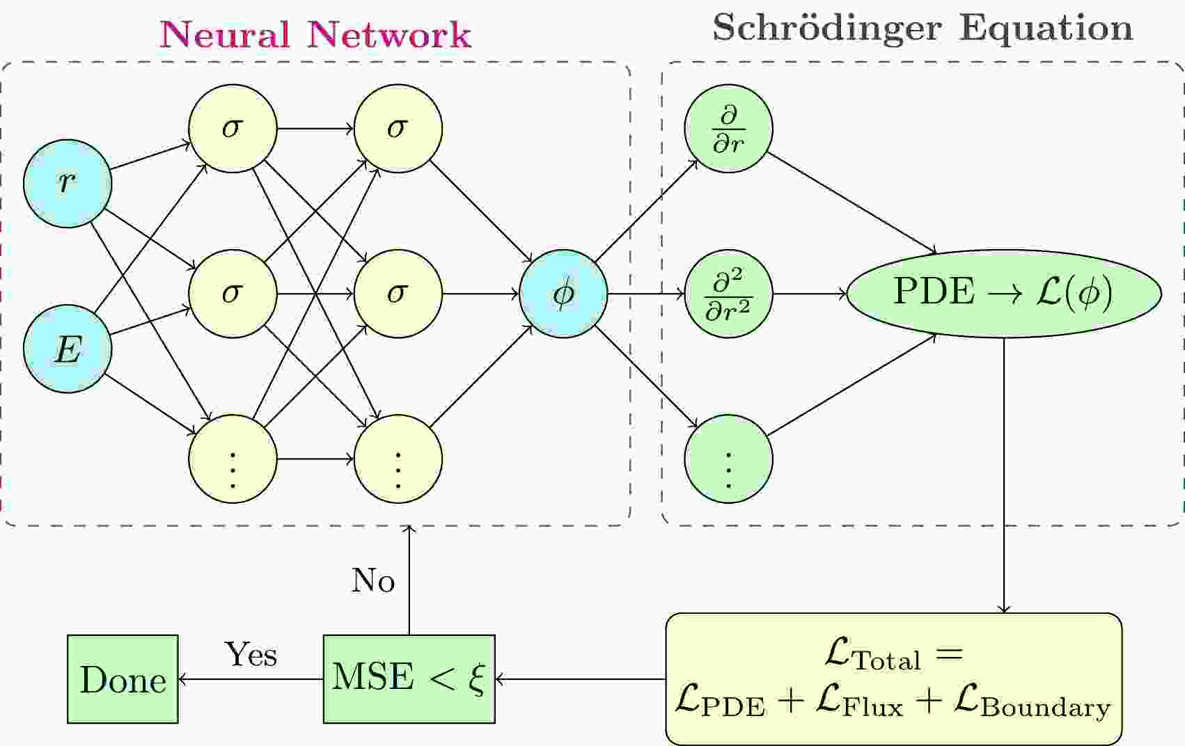
Physics-Informed Neural Networks (PINNs) provide an alternative approach by approximating the solution $ \phi_\theta(r) $ using a neural network [28], where θ represents the set of all trainable parameters (e.g., weights and biases). The key idea is to incorporate the physical laws governing the system directly into the loss function used to train the neural network.

The neural network employed in this study consists of multiple fully connected layers. The input layer receives the spatial coordinates r and incident energy E, while the output layer produces the approximated wavefunction for each channel. A schematic diagram of the adopted physics-informed neural network is shown in Fig. 1. Complex-valued outputs are handled by treating the real and imaginary parts separately.

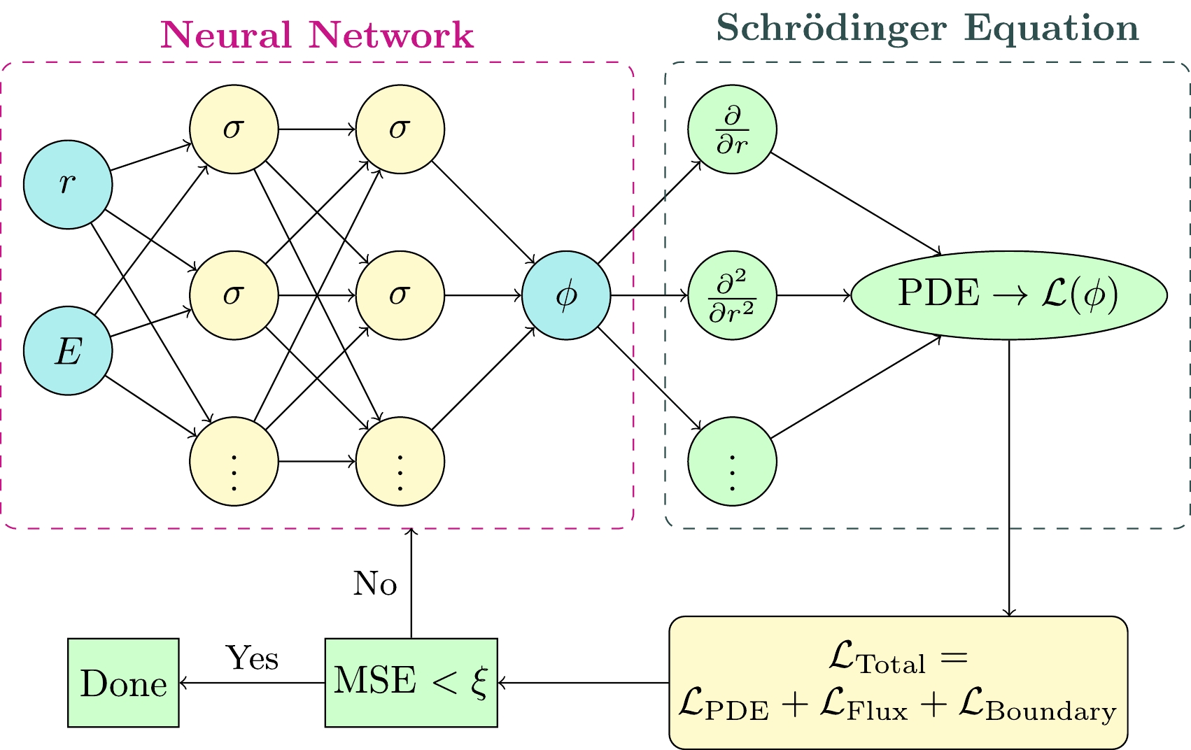
Figure 1.  (color online) Schematic diagram of the adopted physics-informed neural network.

The SIREN (Sinusoidal Representation Networks) activation function is particularly effective for learning functions with high-frequency components [37]. The neurons are combination of $ \sigma(r) = \sin(\omega_0 r + b), $ where $ \omega_0 $ is the frequency parameter and b is a bias term. Proper initialization is critical for training networks with periodic activation. Initialization schemes have been shown to be crucial in the training procedure of deep neural networks, and the weights here are initialized using the special uniform distribution as the same as in Ref. [37].

The key advantage of SIREN lies in the property that its derivatives remain compositions of SIRENs. This is due to the fact that the derivative of the sine function is the cosine function, which is itself a phase-shifted sine wave. Unlike conventional activation functions such as the hyperbolic tangent (tanh) or the rectified linear unit (ReLU), the sine function is periodic. This periodicity, combined with the smooth and continuous nature of sinusoidal activation, enables SIRENs to effectively model complex, high-frequency patterns and fine-grained details. Empirical evidence demonstrates that this unique characteristic of SIRENs significantly enhances their representational capacity, particularly in tasks requiring precise modeling of signals, images, or physical phenomena.

The loss function in the neural network training incorporates several physical constraints to ensure that the learned wavefunctions $ \phi_n(r) $ satisfy the Schrödinger equation and the imposed boundary conditions. The first component is the PDE residual loss $ {\cal{L}}_{\text{PDE}} $, which enforces that the wavefunctions satisfy Eq. (1) across the sample domain:

where $ N_s $ is the number of collocation points $ r_i $.

The second component is the boundary derivative loss $ {\cal{L}}_{\text{Boundary}} $, which ensures that the derivatives of the wavefunctions at the boundaries match the expected physical behavior:

The third component is the flux conservation loss $ {\cal{L}}_{\text{Flux}} $, which enforces the conservation of probability flux, ensuring that the total incoming flux equals the sum of reflected and transmitted fluxes across all open channels:

Combining all components, the neural network's objective is to minimize the total loss:

Finally, the wavefunctions for each channel, as well as the reflection and tunneling probabilities, can be obtained by minimizing the total loss. The Adam optimizer with a learning rate scheduler is employed to train the neural network. The training process involves iteratively updating the network parameters to minimize the total loss function.

In the following studies, we present the results of one-dimensional and multi-channel cases, where the network structure is consistent, with the only difference being the number of output neurons corresponding to the number of channels. For example, in the one-dimensional potential case, the network has 2 output neurons (real and imaginary parts of the wavefunction), while in the three-channel potential case, it has 6 output neurons (2 for each of the 3 channels). The PINN architecture and training hyperparameters are described as follows:

1. Network Structure:

- Input Layer: 2 neurons for spatial coordinate r and incident energy E.

- Hidden Layers: 2 fully connected layers with 128 neurons each, using the SIREN activation function.

- Output Layer: $ 2N $ neurons for real and imaginary parts of wavefunctions across N channels (e.g., $ N=1 $ for Eckart potential, $ N=3 $ for three-channel Gaussian potential).

2. Initialization Strategy:

- Weights: For the first layer, the uniform distribution $ {\cal{U}}(-1/d,\ 1/d) $ is used, while for subsequent layers, the weights are initialized from a uniform distribution $ {\cal{U}}(-\sqrt{6/d}/\omega_0,\ \sqrt{6/d}/\omega_0) $, where d is the input dimensionality of each layer and the frequency parameter $ \omega_0 = 30 $.

- Bias Initialization: The biases in all layers were initialized from a uniform distribution $ {\cal{U}}(-1/\sqrt{d}, 1/\sqrt{d}) $.

- Learning Rate: Initial value is $ 10^{-4} $. A dynamic learning rate scheduler was employed to ensure stability during optimization.

The detailed training methodology is as follows:

1. Boundary Wave Function Calculation: The wave function values at boundary points $ r_{\text{min}} $ and $ r_{\text{max}} $ are directly computed from the neural network's output. The derivatives are calculated via automatic differentiation of the neural network outputs with respect to r.

2. Collocation Point Distribution: The collocation points are uniformly sampled across the spatial domain $ [r_{\text{min}}, r_{\text{max}}] $ with $ 2 \times 10^4 $ intervals.

3. Stopping Criteria: Training was terminated when the total loss $ {\cal{L}}_{\text{Total}} $ improvement is smaller than $ 10^{-5} $ for every 3000 epochs.

4. Complex-Valued Outputs: Complex-valued wavefunctions were handled by splitting the output layer into two channels for real and imaginary parts.

The Eckart potential is a well-known one-dimensional potential with an analytical solution [38]. In this subsection, we adopt the same potential form as in our previous work [39]:

where $ V_B $ and $ R_B $ represent the potential barrier height and radius, respectively.

For the case where $ 8\mu V_B/\hbar^2 > 1 $, the analytical solution for the transmission coefficient is given by:

where $ k = \sqrt{2\mu E/\hbar^2} $. For simplicity, we set $ 2\mu/\hbar^2 = 1 \, \text{MeV}^{-1}\text{fm}^{-2} $, $ R_B = 0 \; \text{fm} $, and $ V_B = 20 \, \text{MeV} $. The shape of the potential is illustrated in Fig. 2.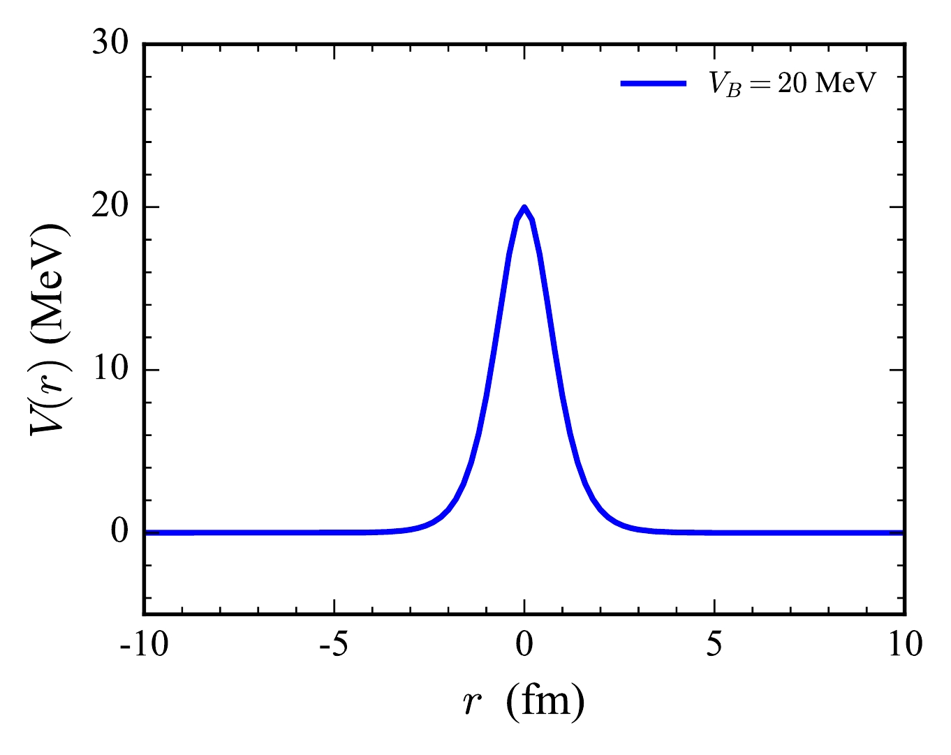

Figure 2.  (color online) The Eckart potential $ V(r) $ from Eq. (10) with $ V_B = 20 \, \text{MeV} $ and $ R_B = 0 \, \text{fm} $.

Fig. 3 compares the tunneling probabilities computed using PINN with the analytical solution. The analytical solution, given by Eq. (11), is represented by the solid line. The close agreement between the PINN results and the analytical solution across both above-barrier and below-barrier energy regions validates the applicability of the PINN approach for this one-channel tunneling problem.

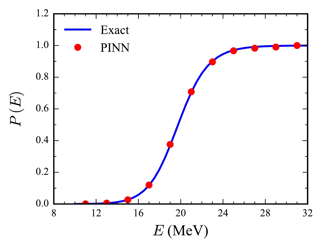
Figure 3.  (color online) Comparison of tunneling probabilities for the Eckart potential between PINN (red circles) and the analytical solution (blue solid line).

The squared modulus of the wavefunction $ |\phi(r)|^2 $ could provide valuable and direct insights into the tunneling probability or the square of tunneling coefficient, based on Eq.(3). The $ |\phi(r)|^2 $ obtained for the one-dimensional Eckart potential under both below-barrier energy $ E = 11 \, \text{MeV} $ and above-barrier energy $ E = 25 \, \text{MeV} $ are given at Fig. 4 and Fig. 5. In each figure, the comparison of the PINN and FEM are shown in panel (a), and the deviations are shown in panel(b). The $ |\phi(r_\text{max})|^2 $ and the tunneling probability tend to be zero in below-barrier energy at Fig. 4 (a), and one in above-barrier energy Fig. 5 (a), respectively. As illustrated in Fig. 4 (a), the squared modulus of the wavefunction $ |\phi(r)|^2 $ exhibits a high degree of oscillation, which is characteristic of quantum tunneling phenomena. Meanwhile, The PINN method accurately captures these oscillations, as evidenced by the close agreement with FEM results shown in panel (a). The deviation plot in panel (b) reveals that the discrepancies between PINN and FEM solutions are minimal, typically within $ 0.01 $. The successful modeling of such features across different energy regimes underscore the capability of PINNs to handle intricate physical phenomena governed by the Schrödinger equation.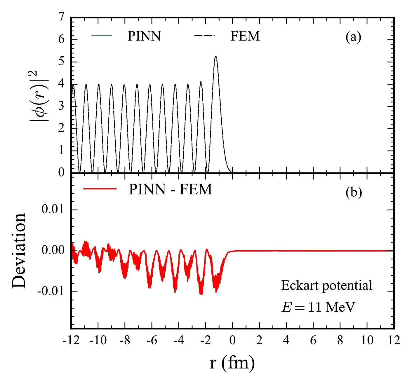

Figure 4.  (color online) Comparison of wavefunction characteristics under the one-dimensional Eckart potential at a below barrier incident energy (E = 11 MeV). (a) Squared modulus of wavefunctions $ ( |\phi(r)|^2 ) $ calculated using PINN and FEM. The solid lines represent the PINN results, while dashed lines denote the FEM solutions. (b) Deviation between the PINN and FEM results represented by the solid line.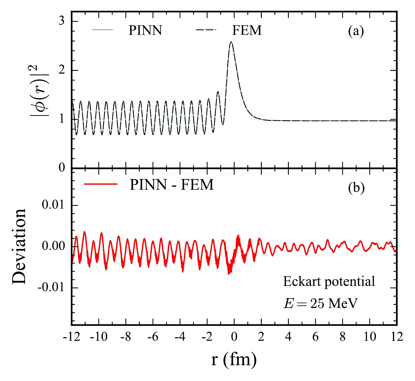

Figure 5.  (color online) Same as Fig. 4, but for the above barrier incident energy (E = 25 MeV) under the one-dimensional Eckart potential.

Next, we consider a three-channel tunneling problem, where the coupling potential is expressed as:

with

where $ V_0 = 100 \, \text{MeV} $, $ F_0 = 3 \, \text{MeV} $, and $ s = s_f = 3 \, \text{fm} $. These parameters are chosen to simulate the potential between two $ ^{58}\text{Ni} $ nuclei. The excitation energy $ \epsilon $ and the reduced mass μ are set to 2 MeV and 29 $ m_N $, respectively, where $ m_N = 938 \, \text{MeV} $ is the nucleon mass. The multidimensional WKB method and the symmetry WKB method have been tested on this three-channel tunneling problem [39, 40].

Due to the lack of an analytical solution, we compare the PINN results with those obtained using high-accuracy FEM based on our recent developed KANTBP program [16], as shown in Fig. 6. The results are presented in both linear (upper panel) and logarithmic (lower panel) scales to highlight the details. In the legend, SC and 3C denote single-channel and three-channel coupling calculations, respectively. The upper panel reveals that the tunneling probability in the three-channel case (3C) is significantly broader compared to the single-channel case (SC). The PINN results closely match the FEM results across the considered energy range. In the logarithmic scale, the tunneling probability in the 3C case is notably enhanced at the sub-barrier energy region due to the presence of coupling, which is shown in the lower panel of this figure. The PINN results remain consistent with the FEM results, demonstrating reliability across probabilities at the considered near barrier energy region.

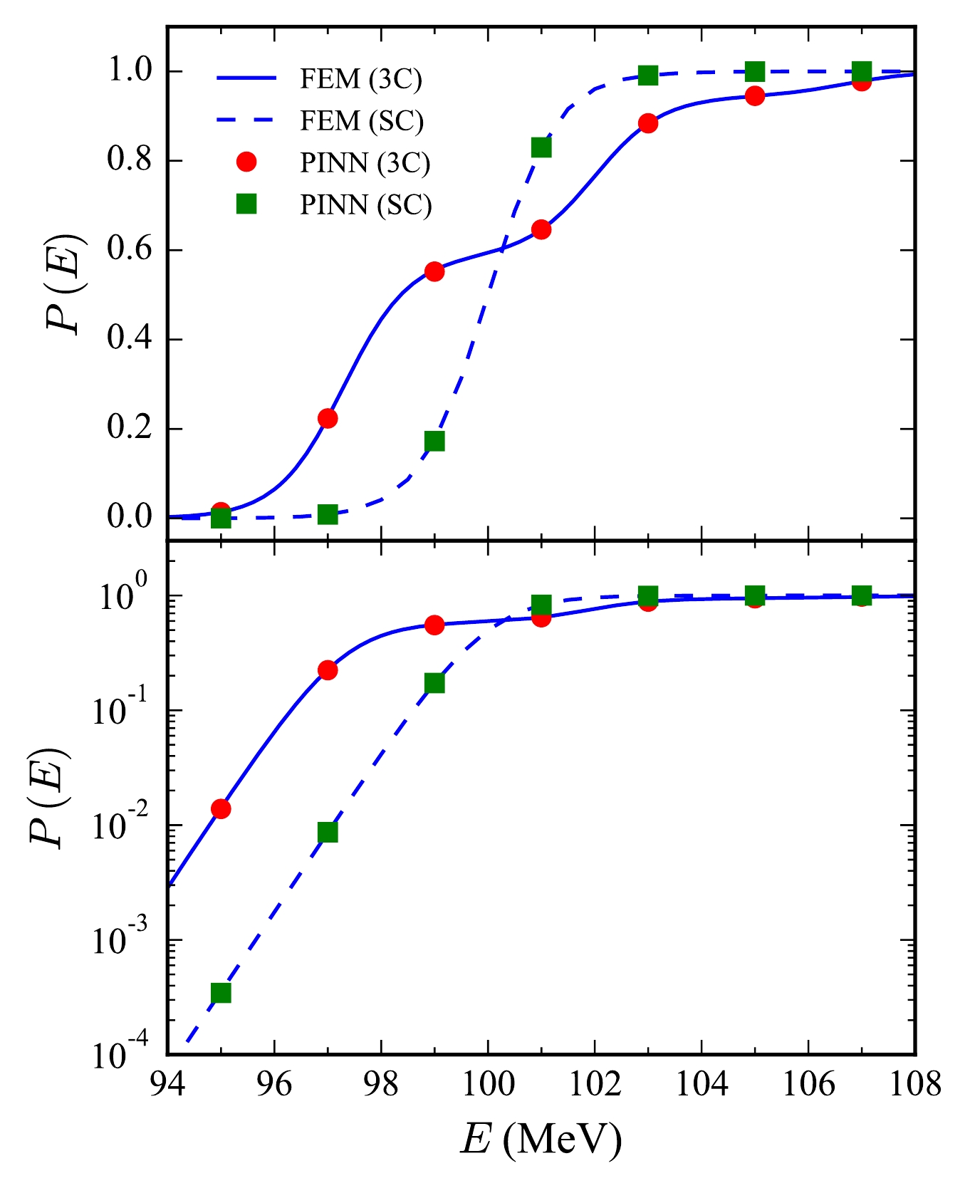
Figure 6.  (color online) Tunneling probability as a function of energy for the three-channel Gaussian potential in linear scale (upper panel) and logarithmic scale (lower panel). SC and 3C represent single-channel and three-channel coupling results, respectively. PINN results are shown as scatter points, and FEM results are shown as lines.

Fig. 7 displays the real and imaginary parts of the wave function computed using PINN at an above barrier energy of $ E = 107.0 \, \text{MeV} $. At this above barrier energy, the tunneling probability is close to 1, and the wave function easily passes through the barrier, as evidenced by the amplitude increase in Channel 1 (upper panel). Due to the high energy relative to the barrier height, the wave function can tunnel into other reaction channels, as seen in the middle and lower panels, where the wave function amplitudes increase significantly after passing the barrier at $ r = 0 $ fm. As evident from the figure, the wave function exhibits substantial oscillations, posing significant challenges for neural network training. Under our testing conditions, only the SIREN neural network successfully learns the correct results, whereas methods such as tanh and ReLU prove to be ineffective.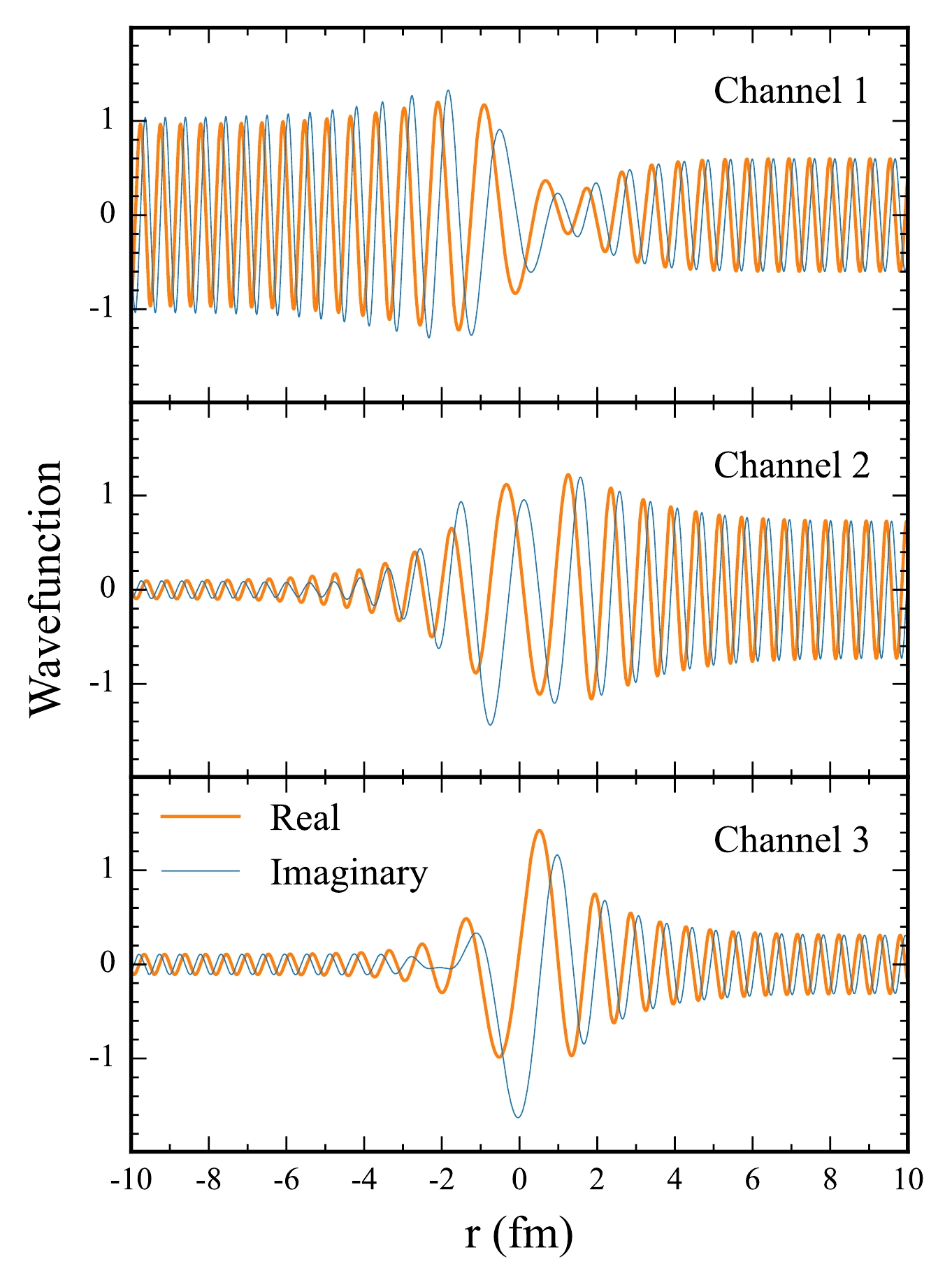

Figure 7.  (color online) Real (thick lines) and imaginary (thin lines) parts of the wave function obtained using PINN for the three-channel Gaussian potential at an above-barrier energy $ E = 107.0 \, \text{MeV} $. The barrier height is 100 MeV, and $ r = 0 $ denotes the barrier position. The wave function is transmitted from left to right.

For the Gaussian potential, the squared modulus of the wavefunction $ |\phi(r)|^2 $ and the deviation computed using PINNs also demonstrate excellent agreement with FEM solutions, as depicted in Figs. 8 and 9. At a below-barrier energy of $ E = 93 \, \text{MeV} $, the wavefunction exhibits pronounced oscillations. The PINN produces near-identical patterns to the FEM results (Fig. 8(a)). The deviation plot (Fig. 8(b)) indicates that the differences between the two methods are negligible. Similarly, at an above-barrier energy of $ E = 103 \, \text{MeV} $, the wavefunction displays a relatively smooth transition through the potential barrier, with the PINN solution closely matching the FEM outcome (Fig. 9(a,b)). These results collectively affirm the reliability of PINNs in solving the Schrödinger equation for potentials with varying shapes.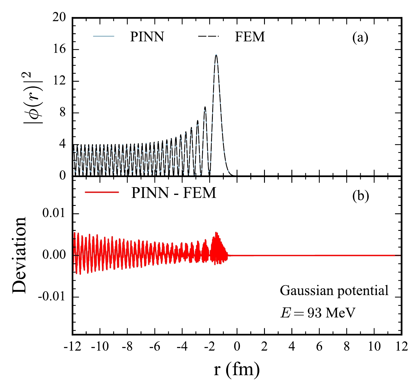

Figure 8.  (color online) Same as Fig. 4, but for the one dimensional Gaussian potential at a below barrier energy $ E=93 $ MeV.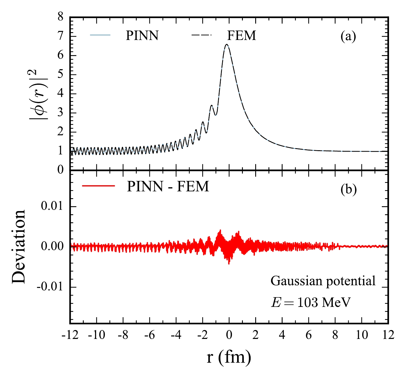

Figure 9.  (color online) Same as Fig. 4, but for the one dimensional Gaussian potential at an above barrier energy $ E=103 $ MeV.

Finally, we examine the training time required for the neural network parameters to converge. Fig. 10 shows the number of epochs needed for different training policies of PINN in the three-channel tunneling case as a function of incident energies. Two training policies are adopted: (1) training with reference to pre-trained wave functions at previous energy point (labeled as "w r"), and (2) training from scratch (labeled as "w/o r"). The results indicate that higher incident energies require more epochs due to the increased momentum and thus oscillations in the wave function. The "w r" training strategy operates through the following protocol. The proceeding of the training could be in either ascending or descending energy order. In current work, we use descending energy order as an example. The neural network trained at energy $ E_i $ serves as the initial parameter set for training at $ E_{i+1} $ with $ E_i > E_{i+1} $. This method preserves learned physical features while allowing adaptation to new energy conditions, meanwhile saving computational resources. The idea of such training strategy is due to that the wavefunctions at adjacent energy points share similar physical features, and only fine-tune is needed for the sequential energy points after the first one. The "w r" policy significantly reduces the number of epochs compared to the "w/o r" policy, demonstrating the advantage of PINN in reusing pre-trained models. This feature is particularly advantageous for calculations involving similar potentials or minor parameter adjustments, such as those required in fusion cross-section or quasi-elastic scattering calculations, where computations across a range of energies and impact parameters are essential. By leveraging pre-trained models, PINNs could reduce the computational burden associated with such batch calculations, enabling more efficient simulations.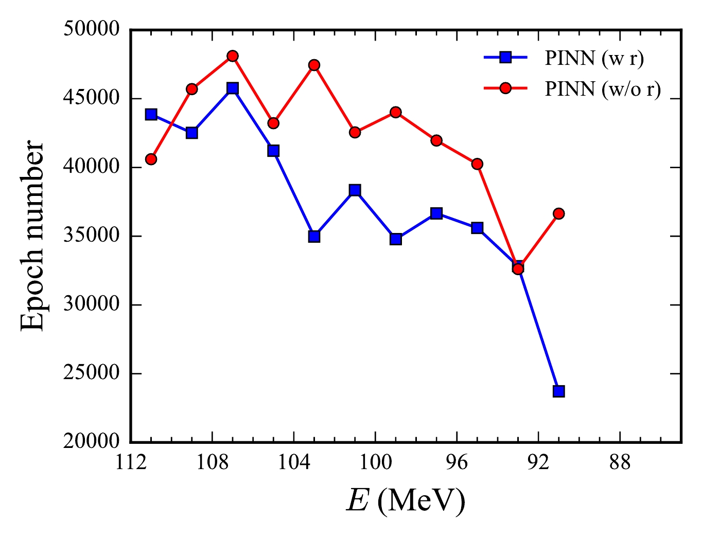

Figure 10.  (color online) Epochs required for different training policies of PINN in the three-channel tunneling case as a function of incident energies. Training with reference to pre-trained wave functions (w r) is represented by squares and solid lines, while training from scratch (w/o r) is represented by circles and dashed lines.

We have presented the first application of PINN to multidimensional quantum tunneling problems using the SIREN activation function to simulate the wavefunction with substantial oscillations. Through examples of the Eckart and three-channel Gaussian potentials, we demonstrated that PINNs achieve results comparable to traditional methods like FEM at the considered near barrier energy region. The study of tunneling in complex and realistic nuclear potentials [41] based on PINN will be addressed in the subsequent works. While the current computational speed of PINN is still much slower compared to FEM, as also shown in Refs. [42, 43], PINNs could be promising in offering significant advantages in high-dimensional problems, where classical methods become computationally prohibitive. Additionally, the ability to save and fine-tune trained neural networks for related calculations reduces computation time. This adaptability allows for rapid reconfiguration of the model to accommodate variations in nuclear properties or reaction conditions without extensive retraining. Future work could explore techniques such as adaptive resampling of collocation points, alternative activation functions, residual connections, and stochastic gradient descent methods to further improve the efficiency of PINNs and tackle the curse of dimensionality [44, 45].

We thank Prof. O. Chuluunbaatar for help on the KANTBP program.