


 Abstract
 HTML
HTML Reference
 Related
 PDF
PDF


-
The Standard Model (SM) is based on the
$S U(3)_{C}\otimes S U(2)_{L}\otimes U(1)_{Y}$ gauge symmetry group and describes the interactions among all elementary particles [1]. The discovery of the Higgs boson by the CMS and ATLAS experiments [2, 3] at the Large Hadron Collider (LHC) in 2012 marks a great success of SM physics. The high-luminosity LHC (HL-LHC), together with other future colliders, such as muon colliders, will not only enable researchers to make more precise measurements on characteristic properties of SM physics but also to unravel undiscovered phenomena beyond SM physics.Recently, a muon collider working at a centre of mass (COM) energy at the TeV scale has received revived interest from the community of high-energy physics [4, 5]. Given that muons are approximately 200 times heavier than electrons, the energy loss caused by synchrotron radiation for muons is much less than that for electrons. Moreover, muon-muon collisions provide a cleaner environment than proton-proton collisions. These features make muon colliders attractive energy-efficient machines to explore high-energy physics.
A muon collider offers numerous opportunities to study elementary particle physics [6, 7]. For instance, when the COM energy is around
$ 1\; {\text{TeV}} $ ,$ \mu^{+}\mu^{-} $ annihilation acts as the dominant production mechanism. At the multi-TeV scale, muons have a high probability to emit electroweak (EW) radiation. Therefore, a high-energy muon collider can also serve as a vector boson collider. Both collision modes provide a spectacular playground for both the search for the origin of EW symmetry breaking (EWSB) and for EW interactions beyond the Standard Model, such as anomalous gauge boson interactions [8−14].For current and future colliders, multi-boson production is an interesting topic, sensitive to the non-abelian character of the SM [1, 15]. In particular, the presence of anomalous quartic gauge boson interactions [16−18] can be probed through tri-boson production and through di-boson production via vector boson scattering. Many studies have been published on this topic at the LHC [19, 20]. In this study, we focussed on two examples, i.e.,
$ {\text{Z}} {\text{Z}} {\text{Z}} $ direct productions through$ \mu^{+}\mu^{-} $ annihilation at a$ 1\; {\text{TeV}} $ muon collider, and$ {\text{Z}} {\text{Z}} $ productions through the VBS process at a$ 10\; {\text{TeV}} $ muon collider, with an integrated luminosity of$ 10\; \text{ab}^{-1} $ . -
Precision measurements of multi-boson production allow a basic test of the SM and provide a model-independent method to search for BSM at the
$ {\text{TeV}} $ scale [19]. In this study, we focussed on$ {\text{Z}} {\text{Z}} {\text{Z}} $ direct productions and$ {\text{Z}} {\text{Z}} $ productions through vector boson scattering. Both processes are sensitive to non-abelian gauge boson interactions and the structure of EW symmetry breaking. These multi-boson processes represent an important avenue to test anomalous triple gauge couplings (aTGCs) and anomalous quartic gauge couplings (aQGCs) [1], as well as to search for possible modifications of these vertices from new physics [20].Anomalous modifications of gauge couplings can be parameterized through the effective field theory (EFT) by adding higher order modifications to the SM Lagrangian:
$ \begin{align} {\cal{L}}^{NP}={\cal{L}}^{4(SM)}+\frac{1}{\Lambda}{\cal{L}}^{5}+\frac{1}{\Lambda^2}{\cal{L}}^{6}+\frac{1}{\Lambda^3}{\cal{L}}^{7}+\frac{1}{\Lambda^4}{\cal{L}}^{8}+... \end{align} $

(1) The higher order terms are suppressed by mass scale Λ, which represents the scale of new physics beyond the SM. The terms featuring odd dimensions are not considered because they will not influence multi-boson production measurements. The dimension-6 operators are related to aTGCs, whereas the dimension-8 operators are related to aQGCs.
Note that aQGCs can be realized by introducing new heavy bosons, which contribute to aQGCs at the tree level, while one loop is suppressed in aTGCs [16, 21, 22]. Furthermore, given that numerous experimental tests of aTGCs have shown good agreement with the SM, this study mainly focused on genuine aQGCs.
To express the aQGC contributions in a model-independent manner, an EFT of the EW breaking sector [16, 23−27] is utilized. When
$S U(2)_{L}\otimes U(1)_{Y}$ is represented linearly, the lowest order genuine aQGC operators parameterized in the EFT are dimension-8 (dim-8) [25, 27−29]. The genuine aQGC operators can be expressed as follows [30]:$ \begin{array}{lc} {\cal O}_{S,0} = \left [ \left ( D_\mu \Phi \right)^\dagger D_\nu \Phi \right ] \times \left [ \left ( D^\mu \Phi \right)^\dagger D^\nu \Phi \right ] , \\ {\cal O}_{S,1} = \left [ \left ( D_\mu \Phi \right)^\dagger D^\mu \Phi \right ] \times \left [ \left ( D_\nu \Phi \right)^\dagger D^\nu \Phi \right ] , \\ {\cal O}_{S,2} = \left [ \left ( D_\mu \Phi \right)^\dagger D_\nu \Phi \right ] \times \left [ \left ( D^\nu \Phi \right)^\dagger D^\mu \Phi \right ] , \\ {\cal O}_{M,0} = \hbox{Tr}\left [ \widehat{W}_{\mu\nu} \widehat{W}^{\mu\nu} \right ] \times \left [ \left ( D_\beta \Phi \right)^\dagger D^\beta \Phi \right ] , \\ {\cal O}_{M,1} = \hbox{Tr}\left [ \widehat{W}_{\mu\nu} \widehat{W}^{\nu\beta} \right ] \times \left [ \left ( D_\beta \Phi \right)^\dagger D^\mu \Phi \right ] , \\ {\cal O}_{M,2} = \left [ B_{\mu\nu} B^{\mu\nu} \right ] \times \left [ \left ( D_\beta \Phi \right)^\dagger D^\beta \Phi \right ]\\ {\cal O}_{M,3} = \left [ B_{\mu\nu} B^{\nu\beta} \right ] \times \left [ \left ( D_\beta \Phi \right)^\dagger D^\mu \Phi \right ] , \\ {\cal O}_{M,4} = \left [ \left ( D_\mu \Phi \right)^\dagger \widehat{W}_{\beta\nu} D^\mu \Phi \right ] \times B^{\beta\nu} , \\ {\cal O}_{M,5} = \left [ \left ( D_\mu \Phi \right)^\dagger \widehat{W}_{\beta\nu} D^\nu \Phi \right ] \times B^{\beta\mu}+ {\rm h.c.} , \end{array} $

$\begin{aligned}[b] \begin{array}{lc} {\cal O}_{M,7} = \left [ \left ( D_\mu \Phi \right)^\dagger \widehat{W}_{\beta\nu} \widehat{W}^{\beta\mu} D^\nu \Phi \right ] ,\\ {\cal O}_{T,0} = \hbox{Tr}\left [ \widehat{W}_{\mu\nu} \widehat{W}^{\mu\nu} \right ] \times \hbox{Tr}\left [ \widehat{W}_{\alpha\beta} \widehat{W}^{\alpha\beta} \right ] , \\ {\cal O}_{T,1} = \hbox{Tr}\left [ \widehat{W}_{\alpha\nu} \widehat{W}^{\mu\beta} \right ] \times \hbox{Tr}\left [ \widehat{W}_{\mu\beta} \widehat{W}^{\alpha\nu} \right ] , \\ {\cal O}_{T,2} = \hbox{Tr}\left [ \widehat{W}_{\alpha\mu} \widehat{W}^{\mu\beta} \right ] \times \hbox{Tr}\left [ \widehat{W}_{\beta\nu} \widehat{W}^{\nu\alpha} \right ] , \\ {\cal O}_{T,3} = \hbox{Tr}\left [ \widehat{W}_{\mu\nu} \widehat{W}_{\alpha\beta} \right ] \times \hbox{Tr}\left [ \widehat{W}^{\alpha\nu} \widehat{W}^{\mu\beta} \right ] , \\ {\cal O}_{T,4} = \hbox{Tr}\left [ \widehat{W}_{\mu\nu} \widehat{W}_{\alpha\beta} \right ] \times B^{\alpha\nu} B^{\mu\beta} , \\ {\cal O}_{T,5} = \hbox{Tr}\left [ \widehat{W}_{\mu\nu} \widehat{W}^{\mu\nu} \right ] \times B_{\alpha\beta} B^{\alpha\beta} , \\ {\cal O}_{T,6} = \hbox{Tr}\left [ \widehat{W}_{\alpha\nu} \widehat{W}^{\mu\beta} \right ] \times B_{\mu\beta} B^{\alpha\nu} , \\ {\cal O}_{T,7} = \hbox{Tr}\left [ \widehat{W}_{\alpha\mu} \widehat{W}^{\mu\beta} \right ] \times B_{\beta\nu} B^{\nu\alpha} , \\ {\cal O}_{T,8} = B_{\mu\nu} B^{\mu\nu} B_{\alpha\beta} B^{\alpha\beta} , \\ {\cal O}_{T,9} = B_{\alpha\mu} B^{\mu\beta} B_{\beta\nu} B^{\nu\alpha} . \end{array} \end{aligned} $

(2) Here, Φ denotes the Higgs doublet, the covariant derivative is given by
$D_\mu \Phi = \left(\partial_\mu + {\rm i} g W^j_\mu \dfrac{\sigma^j}{2} + {\rm i} g^\prime B_\mu \dfrac{1}{2} \right) \Phi$ ,$ \sigma^j $ ($j= 1,2,3$ ) represents the Pauli matrices,$ \widehat{W}_{\mu\nu} \equiv W^j_{\mu\nu} \frac{\sigma^j}{2} $ is the$S U(2)_L$ field strength, and$ B_{\mu\nu} $ denotes the$ U(1)_Y $ one. The effective Lagrangian with the contributions from genuine aQGC operators can be expressed as follows:$ \begin{align} \begin{array}{ll} {\cal{L}}_{\rm eff} &={\cal{L}}_{SM}+{\cal{L}}_{\rm anomalous} \\ &={\cal{L}}_{SM}+ \displaystyle\sum_{d>4} \displaystyle\sum_{i} \dfrac{f_{i}^{(d)}}{\Lambda^{d-4}} O_{i}^{(d)} \\ &={\cal{L}}_{SM}+ \displaystyle\sum_{i} \left[\dfrac{f_{i}^{(6)}}{\Lambda^{2}}O_{i}^{(6)}\right]+ \displaystyle\sum_{j}\left[\dfrac{f_{j}^{(8)}}{\Lambda^{4}}O_{i}^{(8)}\right]+..., \end{array} \end{align} $

(3) where Λ is the characteristic scale and
$f_{j}^{(8)}/\Lambda^{4}= f_{S, j}/\Lambda^{4}, f_{M, j}/\Lambda^{4},\; f_{T, j}/\Lambda^{4}$ represents the coefficients of the corresponding aQGC operators [27]. These coefficients are expected to be zero in the SM prediction.In this study, we are interested in multi-Z productions, which are rare processes yet to be observed. BSM may introduce measurable contributions and result in deviations from the SM prediction. Examples of processes related to
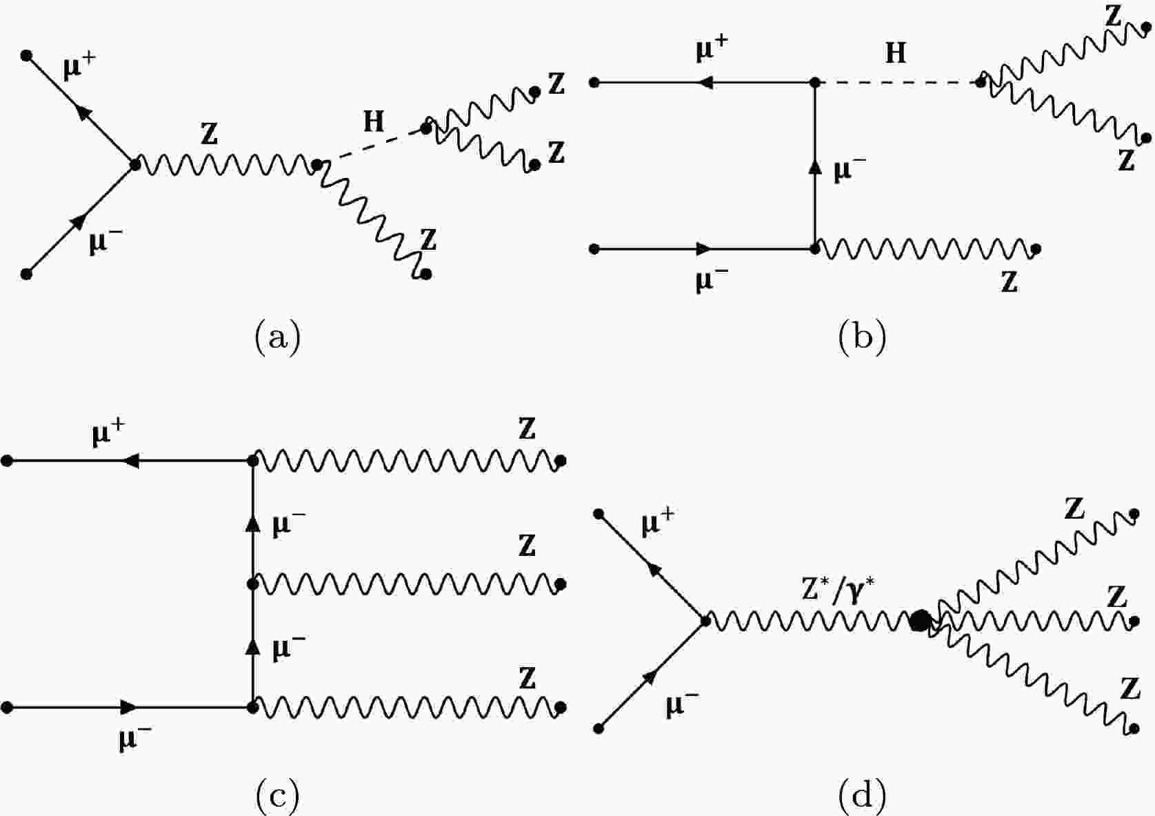
$ {\text{Z}} {\text{Z}} {\text{Z}} $ production in the SM and from the aQGC operator are depicted in Fig. 1, while those for VBS$ {\text{Z}} {\text{Z}} $ production are shown in Fig. 2.
Figure 1. Examples of Feynman diagrams of
$ {\text{Z}} {\text{Z}} {\text{Z}} $ production processes at a muon collider: (a-c) are from the SM and (d) involves quartic gauge couplings.
Figure 2. Examples of Feynman diagrams of VBS
$ {\text{Z}} {\text{Z}} $ production processes at a muon collider: (a) and (b) are from the SM and (c) involves quartic gauge couplings. -
Both the signal and background events were generated with MadGraph5_aMC@NLO [31, 32] at the parton level. Subsequently, they were showered and hadronized through PYTHIA 8.3 [33]. The effects of aQGC operators were simulated with MadGraph5_aMC@NLO using the Universal FeynRules Output module [34, 35]. The SM processes were simulated with the default SM model. DELPHES [36] version 3.0 was used to simulate detector effects, with settings for a muon collider detector [37]. Jets were clustered from the reconstructed stable particles (except electrons and muons) using FASTJET [38], with the
$ k_{T} $ algorithm having a fixed cone size of$R_{\rm jet} = 0.5$ .Two collider scenarios and benchmarks for multi-Z productions were considered: 1) a COM energy of
$ \sqrt{s} = 1 $ TeV for$ {\text{Z}} {\text{Z}} {\text{Z}} $ direct productions, and 2) a$ 10\, {\text{TeV}} $ scale muon collider, where VBS [39] is the dominant production should be replaced by "mechanism, of which the general VBS Feynman diagram is shown in Fig. 3, which includes our VBS$ {\text{Z}} {\text{Z}} $ signal process. Both scenarios were studied at an integral luminosity of$ 10\, \text{ab}^{-1} $ .
Figure 3. Example of diagram of VBS processes at a muon collider.
In the study of the tri-Z boson production at a muon collider, we focused on either a pure leptonic decay,
$ \mu^{+}\mu^{-} \rightarrow {\text{Z}} {\text{Z}} {\text{Z}} \to \ell_{1}^{+}\ell_{1}^{-}\ell_{2}^{+}\ell_{2}^{-} \nu_{3}\bar{\nu}_{3} $ , or a semi-leptonic decay,$ \mu^{+}\mu^{-} \rightarrow {\text{Z}} {\text{Z}} {\text{Z}} \to \ell_{1}^{+}\ell_{1}^{-} \ell_{2}^{+}\ell_{2}^{-} jj $ , where$ \ell $ denotes the electron or muon and j denotes the jet. In the study of the$ {\text{Z}} {\text{Z}} $ productions through VBS, we considered a pure-leptonic channel,$ \mu^{+}\mu^{-} \rightarrow {\text{Z}} {\text{Z}}\nu_{\mu}\bar{\nu}_{\mu} \rightarrow 4\ell+\nu_{\mu}\bar{\nu}_{\mu} $ , and a semi-leptonic channel,$ \mu^{+}\mu^{-} \rightarrow {\text{Z}} {\text{Z}}\nu_{\mu}\bar{\nu}_{\mu}\rightarrow 2\ell 2j+\nu_{\mu}\bar{\nu}_{\mu} $ . The interference effect was included in our simulations with MadGraph. Backgrounds were classified into several categories:• P1: s-channel processes:
–
$ \mu^{+}\mu^{-}\rightarrow X=at\bar{t}+bV+c {\text{H}} $ , with a, b, c as integers.• P2: VBS processes further divided into [40]:
– P2.1:
$ {\text{W}}^{+} {\text{W}}^{-} $ fusion with two neutrinos in the final state, denoted as$ {\text{W}} {\text{W}}\_{\rm VBS} $ below.– P2.2
$ ZZ/Z\gamma/\gamma\gamma $ fusion with two muons in the final state, denoted as$ {\text{Z}} {\text{Z}}\_{\rm VBS} $ below.– P2.3:
$ {\text{W}}^{\pm} {\text{Z}}/ {\text{W}}^{\pm}\gamma $ fusion with one muon and one neutrino in the final state, denoted as$ {\text{W}} {\text{Z}}\_{\rm VBS} $ below.We list all considered backgrounds in Table 1.
SM process type Selected backgrounds P1: s-channel ${\rm {H} } t\overline{t}, { \rm{Z} } t\overline{t}, {\rm {W} } {\rm {W} } t\overline{t}, \rm { {Z} } { {Z} } { {H} }$ ,

$\rm { {Z} } { {H} } { {H} }, { {W} } { {W} } { {Z} }, { {H} } { {H} }, { {W} } { {W} } { {H} }, { {W} } { {W} } { {W} } { {W} }, { {W} } { {W} } { {Z} } { {H} }, { {W} } { {W} } { {Z} } { {Z} }$ 

P2.1: $ {{W}} {{W}}\_{\rm VBS} $ 

$t\overline{t}, \rm { {W} } { {W} } { {H} }, { {Z} } { {H} } { {H} }, { {Z} } { {Z} } { {H} }$ ,

$\rm { {Z} } { {Z} } { {Z} }, { {W} } { {W} } { {Z} }, { {H} } { {H} }, { {Z} } { {Z} }, { {Z} } { {H} }$ 

P2.2: $ {{Z}} {{Z}}\_{\rm VBS} $ 

${\rm { {W} } { {W} }, { {Z} } { {H} }, { {Z} } { {Z} }}, t\overline{t}, \rm { {Z} }, { {H} }, { {W} } { {W} } { {Z} }$ 

P2.3: $ {{W}} {{Z}}\_{\rm VBS} $ 

$\rm { {W} } { {Z} }, { {W} } { {Z} } { {H} }, { {W} } { {H} }, { {W} } { {W} } { {W} }, { {W} } { {Z} } { {Z} }$ 

Table 1. Summary of the backgrounds of the
$ {\text{Z}} {\text{Z}} {\text{Z}} $ process considered in this study.Multi-Z signals studied herein have a very small cross section, whereas the backgrounds are extremely large. Therefore, it is necessary to apply selections to optimize signal yields, while suppressing backgrounds to a large extent. In this numerical analysis, we implemented the cut-based method. Some loose pre-selections were first applied to suppress events of no interest; subsequently, scans on each discriminating variable were performed to maximize signal sensitivity. In this numerical analysis, cut-based selections were optimized for each signal process.
-
To first suppress events of no interest, several pre-selections were applied: the event must include exactly four leptons with transverse momentum
$p_{{T}, \ell} > 20\; {\text{GeV}}$ , absolute pseudo-rapidity$ |\eta_{\ell}|<2.5 $ , and lepton pair geometrical separation of$ \Delta R_{\ell \ell} \ >0.4 $ , where$\Delta R= \sqrt{(\Delta\phi)^{2}+(\Delta\eta)^{2}}$ ;$ \Delta\phi $ and$ \Delta\eta $ are the azimuthal angle separation and pseudorapidity separation of two particles, respectivly. The four leptons were classified and clustered into two reconstructed bosons$ ( {\text{Z}}_{1}, {\text{Z}}_{2}) $ , with their mass denoted as$ M_{\ell\ell,1}, M_{\ell\ell,2} $ , according to the following clustering algorithm:• Construct all possible opposite sign lepton pair candidates: (
$ \ell_{1}\ell_{2} $ ,$ \ell_{3}\ell_{4} $ ) and ($ \ell_{1}\ell_{4},\ell_{2}\ell_{3} $ ).• Calculate the corresponding mass difference:
$ \begin{align} \Delta{M}_{4 \ell}=|M_{\ell\ell, 1}-M_{Z}|+ | M_{\ell\ell, 2}-M_{Z}|, \end{align} $

(4) • Choose minimum
$ \Delta{M}_{4 \ell} $ as the targeted lepton pairs and define$ M_{\ell\ell, 1} > M_{\ell\ell, 2} $ .The selections for the further optimized signal over backgrounds are listed in Table 2, where variable
$ M_{4\ell} $ denotes the invariant mass of the four charged leptons decaying from two Z bosons;$ M_{\ell\ell, 1} $ and$ M_{\ell\ell, 2} $ are the invariant masses of two leptons decayed from reconstructed$ {\text{Z}}_{1} $ and$ {\text{Z}}_{2} $ ;$ p_{T,4\ell} $ is the transverse momentum of four leptons decaying from two Z bosons;$ p_{T, \ell\ell, 1} $ and$ p_{T, \ell\ell, 2} $ are the transverse momentum of two leptons decayed from reconstructed$ {\text{Z}}_{1} $ and$ {\text{Z}}_{2} $ ;$ \Delta R_{\ell\ell, 1} $ and$ \Delta R_{\ell\ell, 2} $ are the geometrical separations of two leptons decayed from reconstructed$ {\text{Z}}_{1} $ and$ {\text{Z}}_{2} $ ;$ |\eta_{\ell\ell, 1}| $ and$ |\eta_{\ell\ell, 2}| $ are the absolute pseudorapidities of reconstructed$ {\text{Z}}_{1} $ and$ {\text{Z}}_{2} $ ;$p_{T,\ell}^{\rm leading}$ denotes the highest$ p_{T} $ in the transverse momentum of the four charged leptons;${\not {E}_T}$ is the missing transverse energy; and$M_{\rm recoil}$ is the recoil mass of four leptons, which can be calculated asVariables Limits for SM Limits for aQGC $ M_{4\ell} $ 

$[200\; {\text{GeV} },900\; {\text{GeV} }]$ 

$[150\; {\text{GeV} },910\; {\text{GeV} }]$ 

$ M_{\ell\ell, 1} $ 

$[80\; {\text{GeV} },120\; {\text{GeV} }]$ 

$[70\; {\text{GeV} },130\; {\text{GeV} }]$ 

$ M_{\ell\ell, 2} $ 

$[60\; {\text{GeV} },100\; {\text{GeV} }]$ 

$[40\; {\text{GeV} },100\; {\text{GeV} }]$ 

$ p_{T,4\ell} $ 

$[30 {\text{GeV} },480\; {\text{GeV} }]$ 

$[30\; {\text{GeV} },500\; {\text{GeV} }]$ 

$ p_{T, \ell\ell, 1} $ 

$< 500\; {\text{GeV} }$ 

$< 500\; {\text{GeV} }$ 

$ p_{T, \ell\ell, 2} $ 

$< 460\; {\text{GeV} }$ 

$< 500\; {\text{GeV} }$ 

$ \Delta R_{\ell\ell, 1} $ 

$ [0.4,3.3] $ 

$ [0.4,3.1] $ 

$ \Delta R_{\ell\ell, 2} $ 

$ [0.4,3.3] $ 

$ [0.4,3.1] $ 

$ |\eta_{\ell\ell, 1}| $ 

$<2.5 $ 

$<2.5 $ 

$ |\eta_{\ell\ell, 2}| $ 

$<2.5 $ 

$<2.5 $ 

$p_{T, \ell}^{\rm leading}$ 

$[20\; {\text{GeV} },380\; {\text{GeV} }]$ 

$[25\; {\text{GeV} },460\; {\text{GeV} }]$ 

$ \Delta{M}_{4 \ell} $ 

$<20 {\text{GeV}} $ 

$< 50\; {\text{GeV} }$ 

${\not {E}_T}$ 

$[50\; {\text{GeV} },460\; {\text{GeV} }]$ 

$[100\; {\text{GeV} },480\; {\text{GeV} }]$ 

$M_{\rm recoil}$ 

$< 300\; {\text{GeV} }$ 

$[35\; {\text{GeV} },225\; {\text{GeV} }]$ 

Table 2. Event selections for
$ {\text{Z}} {\text{Z}} {\text{Z}} $ in the pure-leptonic channel.$ \begin{align} M_{\rm recoil}=\sqrt{(\sqrt{s}-E)^{2}-P^{2}} .\end{align} $

(5) Here,
$ \sqrt{s} $ is the COM energy and E and P are the sum of the energy and momentum of the detectable daughter particles. In these selections, the SM and aQGC signals were optimized separately. For the SM signal, the efficiencies of the pure-leptonic and semi-leptonic channels were 0.75 and 0.34, respectively; for the aQGC signal, the efficiencies of the pure-leptonic and semi-leptonic channels were 0.82 and 0.40, respectively.Figure 4 shows the typical distributions before all selections, including
$ M_{4\ell} $ ,$ M_{\ell\ell,1} $ ,${\not {E}_T}$ , and$M_{\rm recoil}$ . We found that both$ M_{\ell\ell, i} (i = 1, 2) $ and$M_{\rm recoil}$ can distinguish signals and backgrounds well. For the SM signal, we obtained a significance [41] given by$\sqrt{2((s+b)\ln (1+s/b)-s)} = 0.9\sigma$ , with S and B the denoting signal and background yields, respectively. The yield of the process was calculated by summing up the weights of the selected events, which were obtained from$ \dfrac{\sigma\times{\cal{L}}}{N} $ , where σ is the cross-section of the sample,$ {\cal{L}} $ is the luminosity, and N is the total number of generated events. In these plots, we added curves for non-zero aQGCs, setting$f_{T, 0}/\Lambda^{4} = 100\; {\text{TeV}}^{-4}$ as a benchmark. In general, aQGCs lead to excess at high energy tails.
Figure 4. (color online) Various distributions for the
$ {\text{Z}} {\text{Z}} {\text{Z}} $ direct productions in the pure-leptonic channel at a muon collider of$ \sqrt{s}=1\, {\text{TeV}} $ and${\cal{L}}=10\; \text{ab}^{-1}$ : (a) invariant mass of four leptons,$ M_{4\ell} $ ; (b) invariant mass of two leptons,$ M_{\ell\ell, 1} $ ; (c) missing transverse energy,${\not {E}_T}$ ; and (d) recoil mass of four leptons,$M_{\rm recoil}$ . -
A similar analysis was applied for the semi-leptonic channel,
${\text{Z}} {\text{Z}} {\text{Z}} \rightarrow 4\ell+2{\rm jets}$ . Figure 5 shows the distributions of$ M_{4\ell} $ ,$ M_{\ell\ell, 1} $ , the invariant mass of two jets decayed from the other Z boson,$ M_{jj} $ , and the transverse momentum of the jet pair,$ p_{T,jj} $ .
Figure 5. (color online) Various distributions for the
$ {\text{Z}} {\text{Z}} {\text{Z}} $ direct productions in the semi-leptonic channel at a muon collider of$ \sqrt{s}=1\, {\text{TeV}} $ and${\cal{L}}=10\; \text{ab}^{-1}$ : (a) invariant mass of four leptons,$ M_{4\ell} $ distribution; (b) invariant mass of two leptons,$ M_{\ell\ell, 1} $ ; (c) invariant mass of two jets,$ M_{jj} $ ; and (d) transverse momentum of two jets in final state,$ p_{T,jj} $ distribution.The selections of semi-leptonic channel are listed in Table 3, where
$ \Delta R_{jj} $ is the geometrical separation of two jets;$ |\eta_{jj}| $ is the absolute pseudorapidity of the Z boson reconstructed from two jets; and$ p_{T, j}^{\rm leading} $ denotes the highest value of$ p_{T} $ in the transverse momentum of two jets.Variables Limits for SM Limits for aQGC $ M_{4\ell} $ 

$[200\; {\text{GeV} },840\; {\text{GeV} }]$ 

$[150\; {\text{GeV} },930\; {\text{GeV} }]$ 

$ M_{\ell\ell, 1} $ 

$[80\; {\text{GeV} },120\; {\text{GeV} }]$ 

$[85\; {\text{GeV} },130\; {\text{GeV} }]$ 

$ M_{\ell\ell, 2} $ 

$[60\; {\text{GeV} },100\; {\text{GeV} }]$ 

$[65\; {\text{GeV} },115\; {\text{GeV} }]$ 

$ M_{jj} $ 

$< 150\; {\text{GeV} }$ 

$[30\; {\text{GeV} },150\; {\text{GeV} }]$ 

$ p_{T,4\ell} $ 

$[30\; {\text{GeV} },450\; {\text{GeV} }]$ 

$[30\; {\text{GeV} },480\; {\text{GeV} }]$ 

$ p_{T, \ell\ell, 1} $ 

$< 500\; {\text{GeV} }$ 

$< 480\; {\text{GeV} }$ 

$ p_{T, \ell\ell, 2} $ 

$< 460\; {\text{GeV} }$ 

$< 480\; {\text{GeV} }$ 

$ p_{T, jj} $ 

$< 420\; {\text{GeV} }$ 

$< 500\; {\text{GeV} }$ 

$ \Delta R_{\ell\ell, 1} $ 

$ [0.4,3.1] $ 

$ [0.4,3.3] $ 

$ \Delta R_{\ell\ell, 2} $ 

$ [0.4,3.1] $ 

$ [0.4,3.3] $ 

$ \Delta R_{jj} $ 

$ [0.4,4.0] $ 

$ [0.4,3.5] $ 

$ |\eta_{\ell\ell, 1}| $ 

$<2.5 $ 

$<2.5 $ 

$ |\eta_{\ell\ell, 2}| $ 

$<2.5 $ 

$<2.5 $ 

$ |\eta_{jj}| $ 

$<5.0 $ 

$<5.0 $ 

$p_{T, \ell}^{\rm leading}$ 

$[20\; {\text{GeV} },400\; {\text{GeV} }]$ 

$[20\; {\text{GeV} },420\; {\text{GeV} }]$ 

$p_{T, j}^{\rm leading}$ 

$[30\; {\text{GeV} },480\; {\text{GeV} }]$ 

$[30\; {\text{GeV} },510\; {\text{GeV} }]$ 

$ \Delta{M}_{4 \ell} $ 

$< 20\; {\text{GeV} }$ 

$< 30\; {\text{GeV} }$ 

${\not {E}_T}$ 

$< 100\; {\text{GeV} }$ 

$< 150\; {\text{GeV} }$ 

$M_{\rm recoil}$ 

$< 300\; {\text{GeV} }$ 

$[35\; {\text{GeV} },225\; {\text{GeV} }]$ 

Table 3. Event selections for
$ {\text{Z}} {\text{Z}} {\text{Z}} $ in the semi-leptonic channel.The selections improve the significance of both SM and aQGC signals. With
$ 10\, \text{ab}^{-1} $ of integrated luminosity at$ \sqrt{s}=1\, {\text{TeV}} $ , the expected yields of the SM signal and background after the selections are listed in Table 4; concerning the aQGC benchmark, with$f_{T, 0}/\Lambda^{4} = 100\,\; {\text{TeV}}^{-4}$ , the expected yields of the aQGC signal and background after the selections are listed in Table 5.Channels ( $ \sqrt{s}=1\, {\text{TeV}} $ )

Expected signal yield [events] Expected background yield [events] Pure-leptonic channel 5.18 31.72 Semi-leptonic channel 4.48 5.46 Table 4. Expected yields of the SM signal and background after the selections in the
$ {\text{Z}} {\text{Z}} {\text{Z}} $ direct productions.Channels ( $ \sqrt{s}=1\, {\text{TeV}} $ )

Expected signal yield [events] Expected background yield [events] Pure-leptonic channel 5514.90 56.80 Semi-leptonic channel 6271.79 9.16 Table 5. Expected yields of the aQGC signal and background after the selections in the
$ {\text{Z}} {\text{Z}} {\text{Z}} $ direct productions.After the selections, the significance for this semi-leptonic channel can reach
$ 1.7\sigma $ for the SM signal process. We further combined the pure-leptonic and semi-leptonic channels, resulting in a higher significance of$ 1.9\sigma $ for the SM signal. We also searched for aQGCs, obtaining the constraint range of all coefficients$ f_{S,M,T} $ , listed in Table 10.Coefficient Constraint / $ \text{TeV}^{-4} $ 

$ f_{S, 0}/\Lambda^{4} $ 

$ [-211,366] $ 

$ f_{S, 1}/\Lambda^{4} $ 

$ [-207,364] $ 

$ f_{S, 2}/\Lambda^{4} $ 

$ [-213,364] $ 

$ f_{M, 0}/\Lambda^{4} $ 

$ [-13.2, 30.4] $ 

$ f_{M, 1}/\Lambda^{4} $ 

$ [-36.7, 22.9] $ 

$ f_{M, 2}/\Lambda^{4} $ 

$ [-11.8, 13.0] $ 

$ f_{M, 3}/\Lambda^{4} $ 

$ [-23.1, 20.6] $ 

$ f_{M, 4}/\Lambda^{4} $ 

$ [-26.2, 36.8] $ 

$ f_{M, 5}/\Lambda^{4} $ 

$ [-22.5, 31.5] $ 

$ f_{M, 7}/\Lambda^{4} $ 

$ [-43.3, 69.9] $ 

$ f_{T, 0}/\Lambda^{4} $ 

$ [-4.63, 3.28] $ 

$ f_{T, 1}/\Lambda^{4} $ 

$ [-4.51, 3.34] $ 

$ f_{T, 2}/\Lambda^{4} $ 

$ [-9.38, 5.84] $ 

$ f_{T, 3}/\Lambda^{4} $ 

$ [-9.22, 6.00] $ 

$ f_{T, 4}/\Lambda^{4} $ 

$ [-14.8, 11.5] $ 

$ f_{T, 5}/\Lambda^{4} $ 

$ [-7.01, 5.95] $ 

$ f_{T, 6}/\Lambda^{4} $ 

$ [-7.00, 6.06] $ 

$ f_{T, 7}/\Lambda^{4} $ 

$ [-14.9 ,11.6] $ 

$ f_{T, 8}/\Lambda^{4} $ 

$ [-5.25, 5.04] $ 

$ f_{T, 9}/\Lambda^{4} $ 

$ [-10.4, 9.66] $ 

Table 10. Limits at the 95% CL on the aQGC coefficients for the
$ {\text{Z}} {\text{Z}} {\text{Z}} $ process. -
For the VBS
$ {\text{Z}} {\text{Z}} $ process, we performed simulation studies similar to those for the$ {\text{Z}} {\text{Z}} {\text{Z}} $ process. We considered both pure-leptonic ($ \mu^{+}\mu^{-} \rightarrow {\text{Z}} {\text{Z}}\nu_{\mu}\bar{\nu}_{\mu} \rightarrow 4\ell+\nu_{\mu}\bar{\nu}_{\mu} $ ) and semi-leptonic ($ \mu^{+}\mu^{-} \rightarrow {\text{Z}} {\text{Z}}\nu_{\mu}\bar{\nu}_{\mu}\rightarrow 2\ell 2j+\nu_{\mu}\bar{\nu}_{\mu} $ ) channels. The backgrounds were also divided into P1 (s-channel), P2.1 ($ {\text{W}} {\text{W}}\_{\rm VBS} $ ), P2.2 ($ {\text{Z}} {\text{Z}}\_{\rm VBS} $ ), and P2.3 ($ {\text{W}} {\text{Z}}\_{\rm VBS} $ ). They are listed in Table 6.SM process type Selected backgrounds P1: s-channel $ {\text{W}} {\text{W}}, {\text{Z}} {\text{Z}}, {\text{Z}} {\text{H}}, {\text{H}} {\text{H}}, {\text{Z}} {\text{H}} {\text{H}}, $ 

$ {\text{Z}} {\text{Z}} {\text{Z}}, {\text{Z}} {\text{Z}} {\text{H}}, {\text{W}} {\text{W}} {\text{H}}, {\text{W}} {\text{W}} {\text{Z}}, t\overline{t}, $ 

$ {\text{H}} t\overline{t}, {\text{Z}} t\overline{t}, {\text{W}} {\text{W}} t\overline{t}, {\text{W}} {\text{W}} {\text{W}} {\text{W}}, {\text{W}} {\text{W}} {\text{Z}} {\text{H}}, {\text{W}} {\text{W}} {\text{H}} {\text{H}} $ 

P2.1: $ {\text{W}} {\text{W}}\_{\rm VBS} $ 

$ {\text{W}} {\text{W}}, {\text{Z}} {\text{H}}, {\text{H}} {\text{H}}, $ 

$ {\text{W}} {\text{W}} {\text{H}}, {\text{W}} {\text{W}} {\text{Z}}, {\text{Z}} {\text{Z}} {\text{Z}}, {\text{Z}} {\text{Z}} {\text{H}}, {\text{Z}} {\text{H}} {\text{H}}, t\overline{t}, {\text{Z}}, {\text{H}} $ 

P2.2: $ {\text{Z}} {\text{Z}}\_{\rm VBS} $ 

$ {\text{W}} {\text{W}}, {\text{Z}} {\text{H}}, {\text{Z}} {\text{Z}}, t\overline{t}, {\text{Z}}, {\text{W}} {\text{W}} {\text{H}}, {\text{W}} {\text{W}} {\text{Z}}, {\text{H}}, {\text{H}} {\text{H}}, {\text{Z}} {\text{Z}} {\text{Z}}, {\text{Z}} {\text{Z}} {\text{H}}, {\text{Z}} {\text{H}} {\text{H}} $ 

P2.3: $ {\text{W}} {\text{Z}}\_{\rm VBS} $ 

$ {\text{W}} {\text{Z}}, {\text{W}} {\text{Z}} {\text{H}}, {\text{W}} {\text{H}}, {\text{W}} {\text{W}} {\text{W}}, {\text{W}} {\text{Z}} {\text{Z}} $ 

Table 6. Summary of the backgrounds for the VBS
$ {\text{Z}} {\text{Z}} $ process. -
We applied pre-selections on the channel of
$\mu^{+}\mu^{-}\rightarrow {\text{Z}} {\text{Z}}\nu_{\mu}\bar{\nu}_{\mu}\rightarrow4\ell+\nu_{\mu}\bar{\nu}_{\mu}$ at a muon collider with$\sqrt{s}=10\; {\text{TeV}}$ and${\cal{L}}=10\; \text{ab}^{-1}$ , as in the$ {\text{Z}} {\text{Z}} {\text{Z}} $ analysis. The selections of the pure-leptonic channel are listed in Table 7. The signal efficiency of the selections was 0.23.Variables Limits $ M_{4\ell} $ 

$[1900\; {\text{GeV} },8800\; {\text{GeV} }]$ 

$ M_{\ell\ell, 1} $ 

$[70\; {\text{GeV} },140\; {\text{GeV} }]$ 

$ M_{\ell\ell, 2} $ 

$[70\; {\text{GeV} },140\; {\text{GeV} }]$ 

$ p_{T,4\ell} $ 

$[200\; {\text{GeV} },4000\; {\text{GeV} }]$ 

$ p_{T,\ell\ell,1} $ 

$[320\; {\text{GeV} },2800\; {\text{GeV} }]$ 

$ p_{T,\ell\ell,2} $ 

$[280\; {\text{GeV} },2600\; {\text{GeV} }]$ 

$ \Delta R_{\ell\ell,1} $ 

$ [0.4,1.7] $ 

$ \Delta R_{\ell\ell,2} $ 

$ [0.4,1.7] $ 

$ |\eta_{\ell\ell, 1}| $ 

$<2.5 $ 

$ |\eta_{\ell\ell, 2}| $ 

$<2.5 $ 

$p_{T,\ell}^{\rm leading}$ 

$[200\; {\text{GeV} },3000\; {\text{GeV} }]$ 

$ \Delta{M}_{4 \ell} $ 

$< 70\; {\text{GeV} }$ 

${\not {E}_T}$ 

$[30\; {\text{GeV} },4000\; {\text{GeV} }]$ 

$M_{\rm recoli}$ 

$< 8000\; {\text{GeV} }$ 

Table 7. Event selections for VBS
$ {\text{Z}} {\text{Z}} $ in the pure-leptonic channel.Figure 6 shows the distribution of the invariant mass of four leptons, denoted as
$ M_{4\ell} $ , the invariant mass of two leptons, denoted as$ M_{\ell\ell, 1} $ , the transverse momentum of four leptons in final states, denoted as$ p_{T,4\ell} $ , and the transverse momentum of one lepton pair, denoted as$ p_{T,\ell\ell,1} $ . In these plots, we also added curves for non-zero aQGCs, setting$ f_{T, 0}/\Lambda^{4} = 1\, {\text{TeV}}^{-4} $ as a benchmark.
Figure 6. (color online) Simulation results of VBS
$ {\text{Z}} {\text{Z}} $ in the pure-leptonic channel for$\sqrt{s}=10\; {\text{TeV}}, {\cal{L}}=10\; \text{ab}^{-1}$ : (a) invariant mass of four leptons,$ M_{4\ell} $ distribution; (b) invariant mass of two leptons,$ M_{\ell\ell, 1} $ ; (c) transverse momentum of four leptons,$ p_{T,4\ell} $ distribution; and (d) transverse momentum of two leptons,$ p_{TT,\ell\ell,1} $ distribution. -
The selections in the semi-leptonic channel are listed in Table 8, where
$ M_{2\ell2j} $ is the invariant mass of two leptons and two jets decaying from two Z bosons;$ \Delta{M}_{2\ell2j} $ is the mass difference, defined as follows:Variables Limits $ M_{2\ell2j} $ 

$[2000\; {\text{GeV} },8000\; {\text{GeV} }]$ 

$ M_{\ell\ell} $ 

$[40\; {\text{GeV} },140\; {\text{GeV} }]$ 

$ M_{jj} $ 

$[30\; {\text{GeV} },150\; {\text{GeV} }]$ 

$ p_{T,2\ell2j} $ 

$[500\; {\text{GeV} },8000\; {\text{GeV} }]$ 

$ p_{T,\ell\ell} $ 

$[200\; {\text{GeV} },3000\; {\text{GeV} }]$ 

$ p_{T,jj} $ 

$[400\; {\text{GeV} },4000\; {\text{GeV} }]$ 

$ \Delta R_{\ell\ell} $ 

$ [0.4,1.7] $ 

$ \Delta R_{jj} $ 

$>0.4 $ 

$ |\eta_{\ell}| $ 

$<2.5 $ 

$ |\eta_{j}| $ 

$<5.0 $ 

$p_{T,\ell}^{\rm leading}$ 

$[200\; {\text{GeV} },2500\; {\text{GeV} }]$ 

$p_{T,j}^{\rm leading}$ 

$[200\; {\text{GeV} },3000\; {\text{GeV} }]$ 

$ \Delta{M}_{2\ell2j} $ 

$< 200\; {\text{GeV} }$ 

${\not {E}_T}$ 

$[30\; {\text{GeV} },3500\; {\text{GeV} }]$ 

$M_{\rm recoli}$ 

$[1000\; {\text{GeV} },7000\; {\text{GeV} }]$ 

Table 8. Event selections for VBS
$ {\text{Z}} {\text{Z}} $ in the semi-leptonic channel.$ \begin{align} \Delta{M}_{2\ell2j}=|M_{\ell\ell}-M_{Z}|+ | M_{jj}-M_{Z}|, \end{align} $

(6) The signal efficiency of the selections was 0.033.
Figure 7 shows distributions of the invariant mass of jet pair, denoted as
$ M_{jj} $ , lepton pair mass, denoted as$ M_{\ell\ell} $ , together with the aQGC signal with coefficient$f_{T,0}/\Lambda^{4}= 1\, {\text{TeV}}^{-4}$ .
Figure 7. (color online) Simulation results of VBS
$ {\text{Z}} {\text{Z}} $ in the semi-leptonic channel for$\sqrt{s}=10\; {\text{TeV}}, {\cal{L}}=10\; \text{ab}^{-1}$ : (a) invariant mass of two leptons,$ M_{\ell\ell} $ distribution; and (b) invariant mass of two leptons,$ M_{jj} $ .After applying the above selections, the significance of the aQGC signal was improved. With
$ 10\, \text{ab}^{-1} $ of integrated luminosity at$ \sqrt{s}=10\, {\text{TeV}} $ and aQGC benchmark with$ f_{T, 0}/\Lambda^{4} =1\, {\text{TeV}}^{-4} $ , the expected yields of the aQGC signal and background after the selections are listed in Table 9.Channels ( $ \sqrt{s}=10\, {\text{TeV}} $ )

Expected signal yield [events] Expected background yield [events] Pure-leptonic channel 686.97 0.48 Semi-leptonic channel 315.40 0.15 Table 9. Expected yields of the aQGC signal and background after the selections in the VBS
$ {\text{Z}} {\text{Z}} $ productions.We also obtained the limits of all aQGC coefficients of the VBS
$ {\text{Z}} {\text{Z}} $ process, which are listed in Table 11.Coefficient Constraint / $ \text{TeV}^{-4} $ 

$ f_{S, 0}/\Lambda^{4} $ 

$ [-14, 13] $ 

$ f_{S, 1}/\Lambda^{4} $ 

$ [-5.8, 6.7] $ 

$ f_{S, 2}/\Lambda^{4} $ 

$ [-15, 16] $ 

$ f_{M, 0}/\Lambda^{4} $ 

$ [-1.2, 1.1] $ 

$ f_{M, 1}/\Lambda^{4} $ 

$ [-3.9, 3.7] $ 

$ f_{M, 2}/\Lambda^{4} $ 

$ [-8.0, 8.2] $ 

$ f_{M, 3}/\Lambda^{4} $ 

$ [-3.9, 3.8] $ 

$ f_{M, 4}/\Lambda^{4} $ 

$ [-3.3, 3.2] $ 

$ f_{M, 5}/\Lambda^{4} $ 

$ [-2.9, 3.0] $ 

$ f_{M, 7}/\Lambda^{4} $ 

$ [-8.3, 8.1] $ 

$ f_{T, 0}/\Lambda^{4} $ 

$ [-0.11, 0.082] $ 

$ f_{T, 1}/\Lambda^{4} $ 

$ [-0.14, 0.14] $ 

$ f_{T, 2}/\Lambda^{4} $ 

$ [-0.27, 0.21] $ 

$ f_{T, 3}/\Lambda^{4} $ 

$ [-0.27, 0.22] $ 

$ f_{T, 4}/\Lambda^{4} $ 

$ [-1.1, 0.67] $ 

$ f_{T, 5}/\Lambda^{4} $ 

$ [-0.32, 0.25] $ 

$ f_{T, 6}/\Lambda^{4} $ 

$ [-0.47, 0.42] $ 

$ f_{T, 7}/\Lambda^{4} $ 

$ [-0.89, 0.60] $ 

$ f_{T, 8}/\Lambda^{4} $ 

$ [-0.47, 0.48] $ 

$ f_{T, 9}/\Lambda^{4} $ 

$ [-1.1, 1.0] $ 

Table 11. Limits at the 95% CL on the aQGC coefficients for the VBS
$ {\text{Z}} {\text{Z}} $ process. -
We studied the multi-Z productions of
$ {\text{Z}} {\text{Z}} {\text{Z}} $ at a muon collider with$ \sqrt{s}=1\, {\text{TeV}} $ and$ {\cal{L}}=10\, \text{ab}^{-1} $ . Through detailed simulations and signal background analysis, we obtained a significance for the$ {\text{Z}} {\text{Z}} {\text{Z}} $ direct production in the SM of$ 1.9\sigma $ after combining the results from the pure-leptonic and semi-leptonic channels. We also set the constraints of the aQGC coefficients [42] at 95% CL. High-energy muon colliders are ideal to research VBS processes, such as the VBS$ {\text{Z}} {\text{Z}} $ production process. We presented the distribution of various variables and summarized the constraints of aQGC coefficients. For the$ {\text{Z}} {\text{Z}} {\text{Z}} $ process, the constraints of coefficients at 95% CL are listed in Table 10, whereas for the VBS$ {\text{Z}} {\text{Z}} $ production process, the constraints of the aQGC coefficients at 95% CL are listed in Table 11; the unit is$ {\text{TeV}}^{-4} $ .In the ZZZ direct productions, some operators degenerate, such as
$ f_{S0} $ ,$ f_{S1} $ , and$ f_{S2} $ ;$ f_{T0} $ and$ f_{T1} $ ; and$ f_{T5} $ and$ f_{T6} $ . However, we kept all the constraints in Table 10 for the completeness of the set of operator coefficients.In comparison with existing VBS
$ {\text{Z}} {\text{Z}} $ aQGC constraints from the CMS experiment in LHC, which are based on a data sample of proton-proton collisions at COM = 13$\rm TeV$ with an integrated luminosity of${\cal{L}}= 137\; {\rm fb}^{-1}:f_{T, 0}/\Lambda^{4}:[-0.24,0.22], f_{T, 1}/\Lambda^{4}:[-0.31,0.31],$ $f_{T, 2}/ \Lambda^{4}: [-0.63,0.59]$ [43], our results establish stronger limits:$f_{T, 0}/\Lambda^{4}:\; [-0.11, 0.082],\; f_{T, 1}/\Lambda^{4}:\;[-0.14,0.11],$ $f_{T, 2}/\Lambda^{4}: [-0.27,0.21]$ . -
In this study, we investigated
$ {\text{Z}} {\text{Z}} {\text{Z}} $ productions at a muon collider with$\sqrt{s}=1\, {\text{TeV}}, {\cal{L}}=10\; \text{ab}^{-1}$ and VBS$ {\text{Z}} {\text{Z}} $ productions at$ \sqrt{s}=10\, {\text{TeV}}, {\cal{L}}=10\, \text{ab}^{-1} $ , together with their sensitivities on aQGC coefficients. For these two processes, we focused on pure-leptonic and semi-leptonic channels to find the kinematic features that help to increase the detection potential, such as the distribution of$ M_{\ell\ell} $ in the pure-leptonic channel and$ M_{jj} $ in the semi-leptonic channel. We studied the constraints of all aQGC coefficients at 95% CL. For the$ {\text{Z}} {\text{Z}} {\text{Z}} $ process, we supplemented the existing tri-boson aQGC results, and for some coefficients such as$ f_{T, 0}, f_{T, 1}, f_{T, 2} $ in the VBS$ {\text{Z}} {\text{Z}} $ process, our results establish stronger limits than those from previous results. The results demonstrate a great potential to probe the anomalous interactions of gauge bosons at muon colliders owing to their higher effective collision energy, cleaner final states, and higher probability to emit EW radiation than LHC.
Searches for multi-Z boson productions and anomalous gauge boson couplings at a muon collider
- Received Date: 2024-04-03
- Available Online: 2024-10-15
Abstract: Multi-boson productions can be exploited as novel probes either for standard model precision tests or new physics searches, and have become a popular research topic in ongoing LHC experiments and future collider studies, including those for electron–positron and muon–muon colliders. In this study, we focus on two examples, i.e.,


 DownLoad: