Non-relativistic expansion of single-nucleon Dirac equation: Comparison between Foldy-Wouthuysen transformation andsimilarity renormalization group

Yixin Guo; Haozhao Liang

doi:10.1088/1674-1137/43/11/114105

Chinese Physics C> 2019, Vol. 43> Issue(11) : 114105 DOI: 10.1088/1674-1137/43/11/114105

Non-relativistic expansion of single-nucleon Dirac equation: Comparison between Foldy-Wouthuysen transformation andsimilarity renormalization group

Yixin Guo ^1,2,3 ,
Haozhao Liang ^1,2,,

1.
Department of Physics, Graduate School of Science, The University of Tokyo, Tokyo 113-0033, Japan
2.
RIKEN Nishina Center, Wako 351-0198, Japan
3.
Department of Modern Physics, University of Science and Technology of China, Hefei 230026, China

Abstract
HTML
Reference
Related

PDF

Abstract：
By following the Foldy-Wouthuysen (FW) transformation of the Dirac equation, we derive the exact analytic expression up to the 1/M⁴ order for general cases in the covariant density functional theory. The results are compared with the corresponding ones derived from another novel non-relativistic expansion method, the similarity renormalization group (SRG). Based on this comparison, the origin of the difference between the results obtained with the FW transformation and the SRG method is explored.
- Dirac equation ,
- non-relativistic expansion ,
- Foldy-Wouthuysen transformation ,
- similarity renormalization group

1. Introduction

1. Introduction
2. Theoretical framework
     2.1 Non-relativistic expansion by SRG
     2.2 Non-relativistic expansion with the FW transformation
3. Results and discussion
     3.1 Results for spherical symmetry
     3.2 Comparison between FW and SRG approaches
4. Summary and perspectives

The Foldy-Wouthuysen (FW) transformation, also called the Pryce-Tani-Foldy-Wouthuysen transformation [1−4], was initially formulated around 1950 to describe the non-relativistic limit of relativistic electrons. A great advantage of the FW transformation is the simple form of operators corresponding to classical observables. This transformation for spin-1/2 particles was soon extended to the cases of spin-0 and spin-1 particles [5], and later generalized to the case of arbitrary spins [6]. Recently, the exact form of the exponential FW operator for a particle with an arbitrary spin was given in Ref. [7].

The FW transformation is also an elegant method for non-relativistic expansion of the Dirac equation [8]. One milestone of its applications in atomic physics was that, using the FW transformation in the presence of external fields, the fine structure [9, 10], describing the splitting of spectral lines of atoms due to the electron spin and the relativistic corrections to the non-relativistic Schrödinger equation, was successfully testified [8].

Due to its elegant and powerful scheme, the FW transformation has been applied in very diverse areas, such as electrodynamics [11, 12], atomic physics [13, 14], condensed matter physics [15−17], optics [18−20], acoustics [21], quantum chemistry [22−27], nuclear physics [28, 29], quantum field theory [30], gravity [31−34], in the theory of the weak interaction [35, 36], and even in the scheme of supersymmetric quantum mechanics [37]. In recent years, the FW transformation has also been discussed in a gravitational wave background of the generalized Dirac Hamiltonian in the non-relativistic limit [38−40].

Nevertheless, in most of the above studies and applications of the FW transformation, only the leading-order terms were derived and treated, such as the relativistic correction to the kinetic energy appearing up to the order of $1/M^3$ (with M the bare mass of the particle), and the correction due to the spin-orbit coupling and the Darwin term appearing in the order of $1/M^2$ [8]. Recently, the FW non-relativistic expansions have been carried out up to the order of $1/M^7$ [41], and even $1/M^{14}$ [42]. Nevertheless, such derivations are valid only for a family of potentials with certain properties.

For systems of atomic nuclei, the covariant density functional theory [43−45] is one of the state-of-the-art methodologies. During the past decades, it has achieved great success in describing various nuclear phenomena in both stable and exotic nuclei. In this theoretical framework, the equation of motion for nucleons is described by the Dirac equation which includes not only the strong vector potential $V({ r})$ , but also the strong scalar potential $S({ r})$ , whose typical values are $V({ r})\sim 300$ MeV and $S({ r})\sim -350$ MeV, while the mass of nucleon is $M = 939$ MeV. As a result, the non-relativistic expansion of the single-nucleon Dirac equation is non-trivial, and its high-order terms have to be derived and verified carefully.

In 2012, Guo [46] applied the similarity renormalization group (SRG) [47, 48], instead of the FW transformation, for the non-relativistic expansion of the single-nucleon Dirac equation up to the ${1}/{M^3}$ order for investigating the nuclear pseudospin symmetry [49]. Using the SRG method, the Dirac Hamiltonian is gradually transformed into a diagonal form with the evolution controlled by the flow equation. As a result, the eigenequations for the upper and lower components of the Dirac spinors are decoupled at the end of the flow. Also, the non-relativistic reduced Hamiltonian thus obtained is Hermitian, and can also be expanded into the series in terms of ${1}/{M^i}$ . To achieve the accuracy of single-particle energies at the 0.1 MeV level, we demonstrated recently that the ${1}/{M^4}$ -order terms are needed, and presented a detailed derivation and results in Ref. [50].

Both the FW transformation and the SRG method provide a systematic way to carry out a non-relativistic expansion of the Dirac equation up to an arbitrary order. However, the FW transformation employs finite steps of unitary transformation, while the SRG method employs infinite infinitesimal unitary transformations along the flow. Therefore, it is interesting and important to investigate the similarities and differences between these two approaches.

In this paper, we perform an exact non-relativistic expansion of the single-nucleon Dirac equation up to the $1/M^4$ order by using the FW transformation. We also investigate the difference between such results and those obtained by the SRG method.

The paper is organized as follows. In Section 2.1, the SRG method is first recalled and the expansion up to the $1/M^4$ order is shown. The new expansion up to the same order using the FW transformation in a general case, such as the inclusion of the scalar potential, is derived in Section 2.2. The specific form of the result in spherical symmetry is presented in Section 3.1, and the difference between the SRG and FW results, as well as the origin of the difference, is investigated in Section 3.2. Finally, a summary and perspectives are given in Section 4.

2. Theoretical framework

1. Introduction
2. Theoretical framework
     2.1 Non-relativistic expansion by SRG
     2.2 Non-relativistic expansion with the FW transformation
3. Results and discussion
     3.1 Results for spherical symmetry
     3.2 Comparison between FW and SRG approaches
4. Summary and perspectives

2.1 Non-relativistic expansion by SRG

1. Introduction
2. Theoretical framework
     2.1 Non-relativistic expansion by SRG
     2.2 Non-relativistic expansion with the FW transformation
3. Results and discussion
     3.1 Results for spherical symmetry
     3.2 Comparison between FW and SRG approaches
4. Summary and perspectives

In the theoretical framework of covariant density functional theory [43−45, 51−56], the Dirac Hamiltonian for nucleons reads

$H = { \alpha} \cdot { p} + \beta (M+S) + V,$

(1)

where $\alpha$ and $\beta$ are the Dirac matrices, M is the mass of the nucleon, and S and V are the scalar and vector potentials, respectively. In this section, we recall the technique of SRG [47, 48] and show the results up to the $1/M^4$ order [46, 50].

The basic idea of SRG is that the Dirac Hamiltonian in Eq. (1) is transformed by a unitary operator $U(l)$ as

$H(l) = U(l)HU^{†}(l),\quad H(0) = H,$

(2)

with a flow parameter l. While $U(l)$ is not known explicitly, an anti-Hermitian generator $\eta(l)$ related to $U(l)$ as $\eta(l) = \frac{ {\rm d}U(l)}{ {\rm d}l} U^{†}(l)$ is chosen, and the Hamiltonian $H(l)$ evolves with the differential flow equation

$\frac{ {\rm d}H(l)}{ {\rm d}l} = [\eta(l),H(l)].$

(3)

One of the convenient and appropriate choices of $\eta(l)$ reads [48]

$\eta(l) = [\beta M,H(l)],$

(4)

which transforms the Dirac Hamiltonian into a diagonal form.

For solving Eq. (3), the Hamiltonian is first divided into two parts:

$H(l) = \varepsilon(l)+o(l),$

(5)

according to the commutation and anti-commutation relations with respect to $\beta$ , i.e., $[\varepsilon, \beta] = 0$ and $\{o, \beta\} = 0$ . As a result,

$\frac{ {\rm d}\varepsilon(l)}{ {\rm d}l} = 4M\beta o^2(l), \tag{6a}$

(6a)

$\frac{ {\rm d}o(l)}{ {\rm d}l}= 2M\beta[o(l),\varepsilon(l)], \tag{6b}$

(6b)

with the initial conditions

$\varepsilon(0) = \beta(M+S)+V,\qquad o(0) = { \alpha} \cdot { p}.$

(7)

Equations (6a) and (6b) can then be solved with the expansion into the series of ${1}/{M^i}$ [48], which gives

$\frac{\varepsilon(\lambda)}{M}= \sum\limits_{i = 0}^\infty\frac{\varepsilon_i(\lambda)}{M^i},\tag{8a}$

(8a)

$\frac{o(\lambda)}{M}= \sum\limits_{j = 1}^\infty\frac{o_j(\lambda)}{M^j},\tag{8b}$

(8b)

while the flow parameter is replaced by a dimensionless parameter $\lambda = lM^2$ . The solutions are obtained as [46]

$\varepsilon_n(\lambda) = \varepsilon_n(0) +4\beta\int_0^\lambda\sum \limits_{k = 1}^{n - 1}o_k(\lambda')o_{n-k}(\lambda')\, {\rm d}\lambda',\tag{9a}$

(9a)

$o_n(\lambda) = o_n(0){\rm e}^{-4\lambda} +2\beta {\rm e}^{-4\lambda}\int_0^\lambda\sum \limits_{k = 1}^{n - 1}[{\rm e}^{4\lambda'}o_k(\lambda'),\varepsilon_{n-k}(\lambda')] \, {\rm d}\lambda', \tag{9b}$

(9b)

with the initial conditions,

$\begin{array}{l} \varepsilon_0(0) = \beta,\quad \varepsilon_1(0) = \beta S+V,\quad \varepsilon_n(0) = 0\quad \mbox{if}\quad n\geqslant 2,\\ o_1(0) = { \alpha} \cdot { p},\quad o_n(0) = 0\quad \mbox{if}\quad n\geqslant 2. \end{array}$

(10)

Therefore, at the end of the flow $\lambda \rightarrow \infty$ , all the off-diagonal parts vanish, i.e., $o_n(\infty) = 0$ for all n. The diagonalized Dirac operator up to the $1/M^4$ order is not difficult to obtain as [50]

$\begin{split} {\cal H}_{\rm SRG} =& \varepsilon(\infty) = M\varepsilon_0(\infty)+\varepsilon_1(\infty)+\frac{\varepsilon_2(\infty)}{M}+\frac{\varepsilon_3(\infty)}{M^2} +\frac{\varepsilon_4(\infty)}{M^3}+\frac{\varepsilon_5(\infty)}{M^4}+\cdots\\ =&M\varepsilon_0(0)+\varepsilon_1(0)+\frac{1}{2M}\beta o_1^2(0) +\frac{1}{8M^2}[[o_1(0),\varepsilon_1(0)],o_1(0)] +\frac{1}{32M^3}\beta\Big( {-4o_1^4(0)+[[o_1(0),\varepsilon_1(0)],\varepsilon_1(0)]o_1(0)} \\ & {+o_1(0)[[o_1(0),\varepsilon_1(0)],\varepsilon_1(0)] -2[o_1(0),\varepsilon_1(0)][o_1(0),\varepsilon_1(0)]} \Big) +\frac{1}{128M^4}\Big( {-9[[o_1(0),\varepsilon_1(0)],o_1^3(0)] +3[o_1(0),\varepsilon_1(0)]^2\varepsilon_1(0)} \\ &+3\varepsilon_1(0)[o_1(0),\varepsilon_1(0)]^2 -6[o_1(0),\varepsilon_1(0)]\varepsilon_1(0)[o_1(0),\varepsilon_1(0)]\\ & {+3[o_1(0)[o_1(0),\varepsilon_1(0)]o_1(0),o_1(0) +[[[[o_1(0),\varepsilon_1(0)],\varepsilon_1(0)],\varepsilon_1(0)],o_1(0)]} \Big) +\cdots \end{split}$

(11)

2.2 Non-relativistic expansion with the FW transformation

1. Introduction
2. Theoretical framework
     2.1 Non-relativistic expansion by SRG
     2.2 Non-relativistic expansion with the FW transformation
3. Results and discussion
     3.1 Results for spherical symmetry
     3.2 Comparison between FW and SRG approaches
4. Summary and perspectives

In this section, we perform the exact non-relativistic expansion of the single-nucleon Dirac equation up to the $1/M^4$ order by using the FW transformation for a general case, in particular for the scalar potential.

According to the FW transformation in the presence of external fields [2, 4, 8], the corresponding operators are defined as

$O = { \alpha} \cdot { p},\qquad \varepsilon = \beta S+V,\qquad \Lambda = -\frac{i}{2M}\beta O,$

(12)

where the operators O and $\varepsilon$ satisfy $O \beta = -\beta O$ and $\varepsilon \beta = \beta \varepsilon$ , respectively. The Hamiltonian (1) reads

$\begin{align} H = \beta M+O+\varepsilon. \end{align}$

(13)

Based on the above definitions, the Dirac Hamiltonian is transformed by a unitary operation into [8]

$\begin{split} H' =&{\rm e}^{i\Lambda}H{\rm e}^{-i\Lambda} =H+i[\Lambda,H] +\frac{i^2}{2!}[\Lambda,[\Lambda,H]]\\& +\cdots +\frac{i^n}{n!}[\underbrace{\Lambda,[\Lambda,\cdots,[\Lambda}_n,H]\cdots]] +\cdots \end{split}$

(14)

where

$\begin{split} \frac{i^n}{n!}[\underbrace{\Lambda,[\Lambda,\cdots,[\Lambda}_n,H]\cdots]] =& (-1)^{\textstyle\frac{n(n-1)}{2}}\frac{\beta^n}{n!M^n}(O^n\beta M+O^{n+1} \\& +\frac{1}{2^n}[\underbrace{O,[O,\cdots,[O}_n,\varepsilon]\cdots]]).\end{split}$

(15)

Keeping all the terms up to the $1/M^n$ order, the unitary transformed Hamiltonian reads

$\begin{split} H'_{1/M^n} =& \beta M+\varepsilon+\sum \limits_{k = 1}^{n + 1} (-1)^{\textstyle\frac{(k-1)(k-2)}{2}}\frac{k-1}{k!M^{k-1}}\beta^{k-1}O^{k}\\ &+\sum \limits_{k = 0}^n (-1)^{\textstyle\frac{k(k-1)}{2}}\frac{\beta^k}{2^kk!M^k}[\underbrace{O,[O,\cdots,[O}_k,\varepsilon]\cdots]]. \end{split}$

(16)

For example, the corresponding result up to the $1/M^4$ order is

$\begin{split} H'_{1/M^4} =& \beta M +\varepsilon +\frac{1}{2M}\beta O^2 -\frac{1}{3M^2}O^3 -\frac{1}{8M^3}\beta O^4\\& +\frac{1}{30M^4}O^5 +\frac{1}{2M}\beta[O,\varepsilon] -\frac{1}{8M^2}[O,[O,\varepsilon]] \\& -\frac{1}{48M^3}\beta[O,[O,[O,\varepsilon]]] +\frac{1}{384M^4}[O,[O,[O,[O,\varepsilon]]]]. \end{split}$

(17)

In the unitary transformed Hamiltonian, e.g., Eq. (17), the off-diagonal parts are not zero but raised by one order from O to $\dfrac{1}{2M}\beta[O,\varepsilon]$ (plus higher-order terms). In order to make the off-diagonal parts vanish, more precisely speaking to make them higher than a given order, one should repeat the FW transformation until the accuracy is achieved [8]. For that purpose, the operators O and $\varepsilon$ can be redefined according to Eq. (17), and one has

$\begin{split} \varepsilon' =& \varepsilon +\frac{1}{2M}\beta O^2 -\frac{1}{8M^2}[O,[O,\varepsilon]] -\frac{1}{8M^3}\beta O^4 \\&+\frac{1}{384M^4}[O,[O,[O,[O,\varepsilon]]]], \end{split} \tag{18a}$

(18a)

$\begin{split} O' =&\frac{1}{2M}\beta[O,\varepsilon] -\frac{1}{3M^2}O^3 -\frac{1}{48M^3}\beta[O,[O,[O,\varepsilon]]] \\& +\frac{1}{30M^4}O^5, \end{split}\tag{18b}$

(18b)

$\Lambda' =-\frac{i}{2M}\beta O'. \tag{18c}$

(18c)

The corresponding FW transformation reads

$H'' = {\rm e}^{i\Lambda'} H' {\rm e}^{-i\Lambda'}.$

(19)

It can be seen that the off-diagonal parts in $H''$ are of the order of $1/M^2$ . Therefore, one should repeat this procedure to $H'''''$ to make the off-diagonal parts of the order of $1/M^5$ . Of course, to get the resultant diagonal parts in $H'''''$ up to the $1/M^4$ order, a recursion technique makes the calculation less complicated than it looks.

As a result, the non-relativistic expansion with the FW transformation up to the $1/M^4$ order reads

$\begin{split} {\cal H}_{\rm FW} =&\beta M +\varepsilon +\frac{1}{2M}\beta O^2 -\frac{1}{8M^2}[O,[O,\varepsilon]]-\frac{1}{8M^3}\beta O^4 \\&-\frac{1}{8M^3}\beta[O,\varepsilon][O,\varepsilon] +\frac{1}{384M^4}[O,[O,[O,[O,\varepsilon]]]] \\ &+\frac{1}{12M^4}[O^3,[O,\varepsilon]] +\frac{1}{32M^4}[O,\varepsilon][O,\varepsilon]\varepsilon\\& -\frac{1}{16M^4}[O,\varepsilon]\varepsilon[O,\varepsilon] +\frac{1}{32M^4}\varepsilon[O,\varepsilon][O,\varepsilon]. \end{split}$

(20)

3. Results and discussion

1. Introduction
2. Theoretical framework
     2.1 Non-relativistic expansion by SRG
     2.2 Non-relativistic expansion with the FW transformation
3. Results and discussion
     3.1 Results for spherical symmetry
     3.2 Comparison between FW and SRG approaches
4. Summary and perspectives

3.1 Results for spherical symmetry

1. Introduction
2. Theoretical framework
     2.1 Non-relativistic expansion by SRG
     2.2 Non-relativistic expansion with the FW transformation
3. Results and discussion
     3.1 Results for spherical symmetry
     3.2 Comparison between FW and SRG approaches
4. Summary and perspectives

For the systems with spherical symmetry, i.e., for spherical nuclei, the corresponding radial single-nucleon Dirac equation reads [43−45]

$\left( \begin{array}{*{20}{c}} \Sigma(r)+M & -\dfrac{ {\rm d}}{ {\rm d}r}+\dfrac{\kappa}{r}\\ \dfrac{ {\rm d}}{ {\rm d}r}+\dfrac{\kappa}{r} & \Delta(r)-M \end{array} \right ) \left( \begin{array}{*{20}{c}} G(r) \\ F(r) \end{array} \right ) = E \left( \begin{array}{*{20}{c}} G(r) \\ F(r) \end{array} \right ),$

(21)

where $\kappa$ is a good quantum number defined as $\kappa = \mp\; (j+{1}/{2})$ for $j = l\pm{1}/{2}$ , and $\Sigma(r) = V(r) + S(r)$ and $\Delta(r) = V(r) - S(r)$ are the sum and the difference of the vector and scalar potentials, respectively. The single-particle energy $E = \varepsilon +M$ includes the mass of the nucleon. The operators $\varepsilon$ and O read

$\varepsilon = {\left( \begin{array}{*{20}{c}} \Sigma(r) & 0\\ 0 & \Delta(r) \end{array} \right )},\quad O = {\left( \begin{array}{*{20}{c}} 0 &-\dfrac{ {\rm d}}{ {\rm d}r}+\dfrac{\kappa}{r}\\ \dfrac{ {\rm d}}{ {\rm d}r}+\dfrac{\kappa}{r}& 0 \end{array} \right )}.$

(22)

According to Eq. (20), the Dirac Hamiltonian is transformed by the FW transformation as

${\left( \begin{array}{*{20}{c}} {\cal H}^{\rm (F)}_{\rm FW} + M & O\bigg(\dfrac{1}{M^5}\bigg) \\ O\bigg(\dfrac{1}{M^5}\bigg) & {\cal H}^{\rm (D)}_{\rm FW} - M \end{array} \right)},$

(23)

where the superscripts (F) and (D) represent the components of the Dirac Hamiltonian acting on single-particle states in the Fermi sea and Dirac sea, respectively. It is seen that the off-diagonal parts are not strictly zero, which is different from the results of SRG, but are of higher order than the required one. Focusing on single-particle states in the Fermi sea which correspond to their counterparts in the non-relativistic framework, the explicit expansion of ${\cal H}^{\rm (F)}_{\rm FW}$ up to the $1/M^4$ order is worked out in detail as

${\cal H}^{\rm (F)}_{0, {\rm FW}} = \Sigma(r), \tag{24a}$

(24a)

${\cal H}^{\rm (F)}_{1, {\rm FW}} = \frac{1}{2M}p^2, \tag{24b}$

(24b)

${\cal H}^{\rm (F)}_{2, {\rm FW}} = \frac{1}{8M^2}\left( {-4Sp^2 +4S'\frac{ {\rm d}}{ {\rm d}r} -2\frac{\kappa}{r}\Delta' +\Sigma''} \right),\tag{24c}$

(24c)

$\begin{split} {\cal H}^{\rm (F)}_{3, {\rm FW}} =& \frac{1}{8M^3}\left( {-p^4 +4S^2p^2 -8SS'\frac{ {\rm d}}{ {\rm d}r}-2S\Sigma'' }\right.\\&\left.{+4S\Delta'\frac{\kappa}{r} +\Sigma'\Delta'} \right),\end{split}\tag{24d}$

(24d)

$\begin{split} {\cal H}^{\rm (F)}_{4, {\rm FW}} =&\frac{1}{384M^4}\bigg\{144Sp^4 -288S'p^2\frac{ {\rm d}}{ {\rm d}r} +\left[ {72\Delta'\frac{\kappa}{r}}\right.\\&\left.{-24(4\Sigma''+9S'')-192S^3} \right]p^2 +\left[ {72\Delta'\frac{\kappa}{r^2} }\right.\\&\left.{-72\Delta''\frac{\kappa}{r} +24(3S'''+4\Sigma''') +576S^2S'} \right]\frac{ {\rm d}}{ {\rm d}r} \\ &+\left[ {-12(5\Sigma'\!-\!36S')\frac{\kappa(\kappa+1)}{r^3} \!+\!12(5\Sigma''\!+\!12S'')\frac{\kappa(\kappa+1)}{r^2}}\right.\\&\left.{ -72\Delta'\frac{\kappa}{r^3} +72\Delta''\frac{\kappa}{r^2}} {-36\Delta'''\frac{\kappa}{r} -288S^2\Delta'\frac{\kappa}{r} +33\Sigma'''' }\right.\\&\left.{+144S^2\Sigma'' +24S\Sigma'(2\Sigma'-6\Delta')} \right]\bigg\}, \end{split}\tag{24e}$

(24e)

where

$p^2 = -\frac{ {\rm d}^2}{ {\rm d}r^2}+\frac{\kappa(\kappa+1)}{r^2},$

(25)

and

$\begin{split} p^4 =& \frac{ {\rm d}^4}{ {\rm d}r^4} -2\frac{\kappa(\kappa+1)}{r^2}\frac{ {\rm d}^2}{ {\rm d}r^2} +4\frac{\kappa(\kappa+1)}{r^3}\frac{ {\rm d}}{ {\rm d}r}\\& +\frac{\kappa(\kappa+1)(\kappa+3)(\kappa-2)}{r^4}. \end{split}$

(26)

In contrast, the Dirac Hamiltonian transformed by the SRG method reads

${\left( \begin{array}{*{20}{c}} {\cal H}^{\rm (F)}_{\rm SRG} + M & 0 \\ 0 & {\cal H}^{\rm (D)}_{\rm SRG} - M \end{array} \right)}.$

(27)

Its off-diagonal parts strictly vanish up to infinite order. According to Eqs. (11), the explicit expansion of ${\cal H}^{\rm (F)}_{\rm SRG}$ up to the $1/M^4$ order reads [50]

${\cal H}^{\rm (F)}_{0, {\rm SRG}} = \Sigma(r),\tag{28a}$

(28a)

${\cal H}^{\rm (F)}_{1, {\rm SRG}} = \frac{1}{2M}p^2, \tag{28b}$

(28b)

${\cal H}^{\rm (F)}_{2, {\rm SRG}} = \frac{1}{8M^2}\left( {-4Sp^2 +4S'\frac{ {\rm d}}{ {\rm d}r}-2\frac{\kappa}{r}\Delta' +\Sigma''} \right), \tag{28c}$

(28c)

$\begin{split} {\cal H}^{\rm (F)}_{3, {\rm SRG}} =&\frac{1}{32M^3}\left( {-4p^4 +16S^2p^2-32SS'\frac{ {\rm d}}{ {\rm d}r}-8S\Sigma'' }\right.\\&\left.{+16S\Delta'\frac{\kappa}{r} -2\Sigma'^2 +4\Sigma'\Delta'} \right), \end{split}\tag{28d}$

(28d)

$\begin{split} {\cal H}^{\rm (F)}_{4, {\rm SRG}} =& \frac{1}{128M^4} \bigg\{ 48Sp^4 - 96S'p^2\frac{{\rm d}}{{\rm d}r} \\& +\left[ {24\Delta'\frac{\kappa}{r} - 24(\Sigma''+3S'')}-64S^3 \right] p^2 \\& +\left[ {24\Delta'\frac{\kappa}{r^2} -24\Delta''\frac{\kappa}{r} +24(S'''+\Sigma''')}+192S^2S' \right]\frac{{\rm d}}{ {\rm d}r} \end{split}$

$\begin{split} \\& +\bigg[ {-12(\Sigma'-12S')\frac{\kappa(\kappa+1)}{r^3}}\\ & {+12(\Sigma''+4S'')\frac{\kappa(\kappa+1)}{r^2} -24\Delta'\frac{\kappa}{r^3} +24\Delta''\frac{\kappa}{r^2}} \\& { {-12\Delta'''\frac{\kappa}{r} -96S^2\Delta'\frac{\kappa}{r} +9\Sigma'''' +48S^2\Sigma''}}\\&{{+24S\Sigma'(\Sigma'-2\Delta')} \bigg]} \bigg\}. \end{split} \tag{28e}$

(28e)

3.2 Comparison between FW and SRG approaches

1. Introduction
2. Theoretical framework
     2.1 Non-relativistic expansion by SRG
     2.2 Non-relativistic expansion with the FW transformation
3. Results and discussion
     3.1 Results for spherical symmetry
     3.2 Comparison between FW and SRG approaches
4. Summary and perspectives

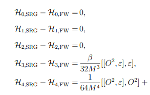
By comparing Eqs. (11) and (20), it is found that

${\cal H}_{0,{\rm SRG}} - {\cal H}_{0,{\rm FW}} =0, \tag{29a}$

(29a)

${\cal H}_{1,{\rm SRG}} - {\cal H}_{1,{\rm FW}} =0, \tag{29b}$

(29b)

${\cal H}_{2,{\rm SRG}} - {\cal H}_{2,{\rm FW}} = 0, \tag{29c}$

(29c)

${\cal H}_{3,{\rm SRG}} - {\cal H}_{3,{\rm FW}} = \frac{\beta}{32M^3}[[O^2,\varepsilon], \varepsilon], \tag{29d}$

(29d)

$\begin{split}{\cal H}_{4,{\rm SRG}} - {\cal H}_{4,{\rm FW}} =&\frac{1}{64M^4}[[O^2,\varepsilon], O^2] \\& +\frac{1}{128M^4}\left[\left([\varepsilon^2,O^2]-2[\varepsilon, O\varepsilon O]\right),\varepsilon\right].\end{split} \tag{29e}$

(29e)

This result seems to indicate that the FW transformation and the SRG method agree with each other up to the $1/M^2$ order, but they lead to different results starting from the $1/M^3$ order. However, considering the infinite mass limit $M \rightarrow \infty$ , all expressions should be strictly organized order by order, and thus the difference between Eqs. (27) and (23) in the $1/M^5$ order cannot lead to the differences of the results in the $1/M^3$ and $1/M^4$ orders. This puzzle needs to be further investigated.

It turns out that the difference shown in Eq. (29) comes from an additional unitary transformation, after the Dirac Hamiltonian is decoupled into the upper and lower parts. Let

$\Xi = -\frac{i\beta}{32M^3}[O^2, \varepsilon] - \frac{i}{128M^4}\left([\varepsilon^2,O^2]-2[\varepsilon, O\varepsilon O]\right).$

(30)

This is a Hermitian and diagonal operator, i.e., $\Xi^{†}= \Xi$ and $\beta\Xi = \Xi\beta$ . Acting an additional unitary transformation on ${\cal H}_{\rm FW}$ , it reads

${\rm e}^{i\Xi}\, {\cal H}_{\rm FW}\, {\rm e}^{-i\Xi} = {\cal H}_{\rm FW} + i [\Xi, {\cal H}_{\rm FW}] + \cdots$

(31)

Keeping all terms up to the $1/M^4$ order, the result is

$\begin{split} {\rm e}^{i\Xi}\, {\cal H}_{\rm FW}\, {\rm e}^{-i\Xi} =&{\cal H}_{\rm FW} + \frac{\beta}{32M^3}[[O^2,\varepsilon], \varepsilon] + \frac{1}{64M^4}[[O^2,\varepsilon], O^2] \\& +\frac{1}{128M^4}\left[\left([\varepsilon^2,O^2]-2[\varepsilon, O\varepsilon O]\right),\varepsilon\right], \end{split}$

(32)

which is nothing else but ${\cal H}_{\rm SRG}$ .

In the spherical case, the explicit expressions for operators $\dfrac{\beta}{32M^3}[[O^2,\varepsilon], \varepsilon]$ , $\dfrac{1}{64M^4}[[O^2,\varepsilon], O^2]$ , and $\dfrac{1}{128M^4}$ $\left[\left([\varepsilon^2,O^2]-2[\varepsilon, O\varepsilon O]\right),\varepsilon\right]$ , acting on single-particle states in the Fermi sea, respectively read

$-\frac{1}{16M^3} {\Sigma'}^2, \tag{33a}$

(33a)

$\frac{1}{64M^4} \left[ {4\Sigma'' p^2 - 4\Sigma'''\frac{\rm d}{{\rm d}r} + 4\Sigma'\frac{\kappa(\kappa+1)}{r^3} - 4\Sigma''\frac{\kappa(\kappa+1)}{r^2} - \Sigma'''' } \right], \tag{33b}$

(33b)

$\frac{1}{16M^4} S {\Sigma'}^2. \tag{33c}$

(33c)

These equations explain the difference between Eqs. (24d) and (28d), as well as between Eqs. (24h) and (28h).

Since ${\rm e}^{-i\Xi}$ is an additional unitary transformation acting on the already decoupled Hamiltonian, it does not affect the non-relativistic expansion of the Dirac equation, and the single-particle spectra obtained by the FW transformation and the SRG method are the same.

The unitary transformation ${\rm e}^{-i\Xi}$ is equivalent to a rotation in a linear and closed complex space, and in quantum mechanics, the operation or rotation in such a space should be associated with a corresponding generator. However, in the present context, it is nontrivial to write down a general expression for such a generator, or derive a conserved quantity that is asymptotically related to a generator up to an arbitrary order. This is because the number of unitary transformations from the FW results to the SRG ones would in principle be infinite, since the SRG method employs infinite infinitesimal unitary transformations along the flow. Therefore, the physics behind the introduced unitary transformation is open for future studies.

4. Summary and perspectives

1. Introduction
2. Theoretical framework
     2.1 Non-relativistic expansion by SRG
     2.2 Non-relativistic expansion with the FW transformation
3. Results and discussion
     3.1 Results for spherical symmetry
     3.2 Comparison between FW and SRG approaches
4. Summary and perspectives

In this work, we investigated the non-relativistic expansion of the single-nucleon Dirac equation in the theoretical framework of covariant density functional theory for a general case where the scalar potential is included. We worked out the exact analytical expansion up to the $1/M^4$ order using the FW transformation. A further investigation of the difference between Eqs. (27) and (23) explained the puzzle that a disagreement seems to appear between the results obtained with the FW transformation and the SRG method, i.e. the non-relativistic expansion of the Dirac equation is affected, but the single-particle spectra obtained by the FW transformation and the SRG method are the same.

The non-relativistic expansion of the Dirac equation for nuclear systems using the FW transformation has been extended to as high orders as needed. Similarly to the SRG method, we anticipate that this novel non-relativistic expansion method will establish in future studies a potential bridge between the relativistic and non-relativistic density functional theories. In particular, with the present FW transformation, all unitary transformations involved are in an explicit form. This leads in a straightforward way to the corresponding transformations of the other relevant operators, such as the one-body density operators.

References

[1]	M. H. L. Pryce and S. Chapman, Proc. Royal Soc. A, 195: 62 (1948) doi: 10.1098/rspa.1948.0103
[2]	L. L. Foldy and S. A. Wouthuysen, Phys. Rev., 78: 29 (1950) doi: 10.1103/PhysRev.78.29
[3]	S. Tani, Prog. Theor. Phys., 6: 267 (1951) doi: 10.1143/ptp/6.3.267
[4]	L. L. Foldy, Phys. Rev., 87: 688 (1952) doi: 10.1103/PhysRev.87.688
[5]	K. M. Case, Phys. Rev., 95: 1323 (1954) doi: 10.1103/PhysRev.95.1323
[6]	J. Jayaraman, J. Phys. A: Math. Gen., 8: L1 (1975) doi: 10.1088/0305-4470/8/1/001
[7]	A. J. Silenko, Phys. Rev. A, 94: 032104 (2016) doi: 10.1103/PhysRevA.94.032104
[8]	W. Greiner, Relativistic Quantum Mechanics Wave Equations (Springer, 1990) pp. 277−290
[9]	A. A. Michelson and E. W. Morley, Philos. Mag. (Series 5), 24: 463 (1887) doi: 10.1080/14786448708628131
[10]	A. Sommerfeld, Sci. Nat., 28: 417 (1940) doi: 10.1007/BF01490583
[11]	A. Y. Silenko, Theor. Math. Phys., 105: 1224 (1995) doi: 10.1007/BF02067491
[12]	A. J. Silenko, J. Math. Phys., 44: 2952 (2003) doi: 10.1063/1.1579991
[13]	M. Hiramoto, T. Fujita, and T. Asaga, Prog. Theor. Phys., 106: 1223 (2001) doi: 10.1143/PTP.106.1223
[14]	K. Pachucki, Phys. Rev. A, 71: 012503 (2005) doi: 10.1103/PhysRevA.71.012503
[15]	K. Y. Bliokh, EPL, 72: 7 (2005) doi: 10.1209/epl/i2005-10205-1
[16]	P. Gosselin, A. Bérard, and H. Mohrbach, Eur. Phys. J. B, 58: 137 (2007) doi: 10.1140/epjb/e2007-00212-6
[17]	P. Gosselin, A. Bérard, H. Mohrbach, and S. Ghosh, Eur. Phys. J. C, 59: 883 (2009) doi: 10.1140/epjc/s10052-008-0839-4
[18]	M. Lippert, T. Bruckel, T. Kohler, and J. R. Schneider, EPL, 27: 537 (1994) doi: 10.1209/0295-5075/27/7/008
[19]	S. A. Khan, Optik, 117: 481 (2006) doi: 10.1016/j.ijleo.2005.11.010
[20]	Y. Hinschberger and P.-A. Hervieux, Phys. Lett. A, 376: 813 (2012) doi: 10.1016/j.physleta.2012.01.023
[21]	L. Fishman, J. Math. Phys., 33: 1887 (1992) doi: 10.1063/1.529666
[22]	M. Reiher, Theor. Chem. Acc., 116: 241 (2006) doi: 10.1007/s00214-005-0003-2
[23]	J. Autschbach, Coord. Chem. Rev., 251: 1796 (2007) doi: 10.1016/j.ccr.2007.02.012
[24]	W. Liu, Mol. Phys., 108: 1679 (2010) doi: 10.1080/00268971003781571
[25]	T. Nakajima and K. Hirao, Chem. Rev., 112: 385 (2012) doi: 10.1021/cr200040s
[26]	D. Peng and M. Reiher, J. Chem. Phys., 136: 244108 (2012) doi: 10.1063/1.4729788
[27]	D. Peng and M. Reiher, Theor. Chem. Acc., 131: 1081 (2012) doi: 10.1007/s00214-011-1081-y
[28]	H. Arodź and K. Golec, Phys. Rev. D, 33: 534 (1986) doi: 10.1103/PhysRevD.33.534
[29]	S. Scherer, G. Poulis, and H. Fearing, Nucl. Phys. A, 570: 686 (1994) doi: 10.1016/0375-9474(94)90079-5
[30]	V. P. Neznamov, Phys. Part. Nucl., 37: 86 (2006) doi: 10.1134/S1063779606010023
[31]	A. J. Silenko and O. V. Teryaev, Phys. Rev. D, 71: 064016 (2005) doi: 10.1103/PhysRevD.71.064016
[32]	P. Gosselin and H. Mohrbach, Eur. Phys. J. C, 71: 1739 (2011) doi: 10.1140/epjc/s10052-011-1739-6
[33]	Y. N. Obukhov, A. J. Silenko, and O. V. Teryaev, Phys. Rev. D, 88: 084014 (2013) doi: 10.1103/PhysRevD.88.084014
[34]	Y. N. Obukhov, A. J. Silenko, and O. V. Teryaev, Phys. Rev. D, 90: 124068 (2014) doi: 10.1103/PhysRevD.90.124068
[35]	A. J. Silenko, Nucl. Instrum. Methods Phys. Res. Sect. B, 114: 259 (1996) doi: 10.1016/0168-583X(96)00212-1
[36]	A. J. Silenko, Theor. Math. Phys., 112: 922 (1997) doi: 10.1007/BF02634108
[37]	G. Junker and A. Inomata, J. Math. Phys., 59: 052301 (2018) doi: 10.1063/1.5020545
[38]	B. Gonçalves, Y. N. Obukhov, and I. L. Shapiro, Phys. Rev. D, 75: 124023 (2007) doi: 10.1103/PhysRevD.75.124023
[39]	J. Q. Quach, Phys. Rev. D, 92: 084047 (2015) doi: 10.1103/PhysRevD.92.084047
[40]	J. Q. Quach, Phys. Rev. D, 93: 104048 (2016) doi: 10.1103/PhysRevD.93.104048
[41]	T.-W. Chen and D.-W. Chiou, Phys. Rev. A, 82: 012115 (2010) doi: 10.1103/PhysRevA.82.012115
[42]	T.-W. Chen and D.-W. Chiou, Phys. Rev. A, 90: 012112 (2014) doi: 10.1103/PhysRevA.90.012112
[43]	J. Meng, H. Toki, S. Zhou et al, Prog. Part. Nucl. Phys., 57: 470 (2006) doi: 10.1016/j.ppnp.2005.06.001
[44]	J. Meng and S. G. Zhou, J. Phys. G: Nucl. Part. Phys., 42: 093101 (2015) doi: 10.1088/0954-3899/42/9/093101
[45]	J. Meng, ed., Relativistic Density Functional for Nuclear Structure (World Scientific, 2016)
[46]	J.-Y. Guo, Phys. Rev. C, 85: 021302 (2012) doi: 10.1103/PhysRevC.85.021302
[47]	F. Wegner, Ann. Phys. (Berl.), 506: 77 (1994) doi: 10.1002/andp.19945060203
[48]	A. Bylev and H. Pirner, Phys. Lett. B, 428: 329 (1998) doi: 10.1016/S0370-2693(98)00417-1
[49]	H. Liang, J. Meng, and S.-G. Zhou, Phys. Rep., 570: 1 (2015) doi: 10.1016/j.physrep.2014.12.005
[50]	Y. Guo and H. Liang, Phys. Rev. C, 99: 054324 (2019) doi: 10.1103/PhysRevC.99.054324
[51]	Y. Chen, L. Li, H. Liang et al, Phys. Rev. C, 85: 067301 (2012) doi: 10.1103/PhysRevC.85.067301
[52]	W. Zhang and Y.-F. Niu, Chin. Phys. C, 41: 094102 (2017) doi: 10.1088/1674-1137/41/9/094102
[53]	Z. Xu and Z.-P. Li, Chin. Phys. C, 41: 124107 (2017) doi: 10.1088/1674-1137/41/12/124107
[54]	Y.-Y. Zong and B.-Y. Sun, Chin. Phys. C, 42: 024101 (2018) doi: 10.1088/1674-1137/42/2/024101
[55]	R. Swain, S. K. Patra, and B. B. Sahu, Chin. Phys. C, 42: 084102 (2018) doi: 10.1088/1674-1137/42/8/084102
[56]	Z.-Z. Li, S.-Y. Chang, Q. Zhao et al, Chin. Phys. C, 43: 074107 (2019) doi: 10.1088/1674-1137/43/7/074107

References

[1]	M. H. L. Pryce and S. Chapman, Proc. Royal Soc. A, 195: 62 (1948) doi: 10.1098/rspa.1948.0103
[2]	L. L. Foldy and S. A. Wouthuysen, Phys. Rev., 78: 29 (1950) doi: 10.1103/PhysRev.78.29
[3]	S. Tani, Prog. Theor. Phys., 6: 267 (1951) doi: 10.1143/ptp/6.3.267
[4]	L. L. Foldy, Phys. Rev., 87: 688 (1952) doi: 10.1103/PhysRev.87.688
[5]	K. M. Case, Phys. Rev., 95: 1323 (1954) doi: 10.1103/PhysRev.95.1323
[6]	J. Jayaraman, J. Phys. A: Math. Gen., 8: L1 (1975) doi: 10.1088/0305-4470/8/1/001
[7]	A. J. Silenko, Phys. Rev. A, 94: 032104 (2016) doi: 10.1103/PhysRevA.94.032104
[8]	W. Greiner, Relativistic Quantum Mechanics Wave Equations (Springer, 1990) pp. 277−290
[9]	A. A. Michelson and E. W. Morley, Philos. Mag. (Series 5), 24: 463 (1887) doi: 10.1080/14786448708628131
[10]	A. Sommerfeld, Sci. Nat., 28: 417 (1940) doi: 10.1007/BF01490583
[11]	A. Y. Silenko, Theor. Math. Phys., 105: 1224 (1995) doi: 10.1007/BF02067491
[12]	A. J. Silenko, J. Math. Phys., 44: 2952 (2003) doi: 10.1063/1.1579991
[13]	M. Hiramoto, T. Fujita, and T. Asaga, Prog. Theor. Phys., 106: 1223 (2001) doi: 10.1143/PTP.106.1223
[14]	K. Pachucki, Phys. Rev. A, 71: 012503 (2005) doi: 10.1103/PhysRevA.71.012503
[15]	K. Y. Bliokh, EPL, 72: 7 (2005) doi: 10.1209/epl/i2005-10205-1
[16]	P. Gosselin, A. Bérard, and H. Mohrbach, Eur. Phys. J. B, 58: 137 (2007) doi: 10.1140/epjb/e2007-00212-6
[17]	P. Gosselin, A. Bérard, H. Mohrbach, and S. Ghosh, Eur. Phys. J. C, 59: 883 (2009) doi: 10.1140/epjc/s10052-008-0839-4
[18]	M. Lippert, T. Bruckel, T. Kohler, and J. R. Schneider, EPL, 27: 537 (1994) doi: 10.1209/0295-5075/27/7/008
[19]	S. A. Khan, Optik, 117: 481 (2006) doi: 10.1016/j.ijleo.2005.11.010
[20]	Y. Hinschberger and P.-A. Hervieux, Phys. Lett. A, 376: 813 (2012) doi: 10.1016/j.physleta.2012.01.023
[21]	L. Fishman, J. Math. Phys., 33: 1887 (1992) doi: 10.1063/1.529666
[22]	M. Reiher, Theor. Chem. Acc., 116: 241 (2006) doi: 10.1007/s00214-005-0003-2
[23]	J. Autschbach, Coord. Chem. Rev., 251: 1796 (2007) doi: 10.1016/j.ccr.2007.02.012
[24]	W. Liu, Mol. Phys., 108: 1679 (2010) doi: 10.1080/00268971003781571
[25]	T. Nakajima and K. Hirao, Chem. Rev., 112: 385 (2012) doi: 10.1021/cr200040s
[26]	D. Peng and M. Reiher, J. Chem. Phys., 136: 244108 (2012) doi: 10.1063/1.4729788
[27]	D. Peng and M. Reiher, Theor. Chem. Acc., 131: 1081 (2012) doi: 10.1007/s00214-011-1081-y
[28]	H. Arodź and K. Golec, Phys. Rev. D, 33: 534 (1986) doi: 10.1103/PhysRevD.33.534
[29]	S. Scherer, G. Poulis, and H. Fearing, Nucl. Phys. A, 570: 686 (1994) doi: 10.1016/0375-9474(94)90079-5
[30]	V. P. Neznamov, Phys. Part. Nucl., 37: 86 (2006) doi: 10.1134/S1063779606010023
[31]	A. J. Silenko and O. V. Teryaev, Phys. Rev. D, 71: 064016 (2005) doi: 10.1103/PhysRevD.71.064016
[32]	P. Gosselin and H. Mohrbach, Eur. Phys. J. C, 71: 1739 (2011) doi: 10.1140/epjc/s10052-011-1739-6
[33]	Y. N. Obukhov, A. J. Silenko, and O. V. Teryaev, Phys. Rev. D, 88: 084014 (2013) doi: 10.1103/PhysRevD.88.084014
[34]	Y. N. Obukhov, A. J. Silenko, and O. V. Teryaev, Phys. Rev. D, 90: 124068 (2014) doi: 10.1103/PhysRevD.90.124068
[35]	A. J. Silenko, Nucl. Instrum. Methods Phys. Res. Sect. B, 114: 259 (1996) doi: 10.1016/0168-583X(96)00212-1
[36]	A. J. Silenko, Theor. Math. Phys., 112: 922 (1997) doi: 10.1007/BF02634108
[37]	G. Junker and A. Inomata, J. Math. Phys., 59: 052301 (2018) doi: 10.1063/1.5020545
[38]	B. Gonçalves, Y. N. Obukhov, and I. L. Shapiro, Phys. Rev. D, 75: 124023 (2007) doi: 10.1103/PhysRevD.75.124023
[39]	J. Q. Quach, Phys. Rev. D, 92: 084047 (2015) doi: 10.1103/PhysRevD.92.084047
[40]	J. Q. Quach, Phys. Rev. D, 93: 104048 (2016) doi: 10.1103/PhysRevD.93.104048
[41]	T.-W. Chen and D.-W. Chiou, Phys. Rev. A, 82: 012115 (2010) doi: 10.1103/PhysRevA.82.012115
[42]	T.-W. Chen and D.-W. Chiou, Phys. Rev. A, 90: 012112 (2014) doi: 10.1103/PhysRevA.90.012112
[43]	J. Meng, H. Toki, S. Zhou et al, Prog. Part. Nucl. Phys., 57: 470 (2006) doi: 10.1016/j.ppnp.2005.06.001
[44]	J. Meng and S. G. Zhou, J. Phys. G: Nucl. Part. Phys., 42: 093101 (2015) doi: 10.1088/0954-3899/42/9/093101
[45]	J. Meng, ed., Relativistic Density Functional for Nuclear Structure (World Scientific, 2016)
[46]	J.-Y. Guo, Phys. Rev. C, 85: 021302 (2012) doi: 10.1103/PhysRevC.85.021302
[47]	F. Wegner, Ann. Phys. (Berl.), 506: 77 (1994) doi: 10.1002/andp.19945060203
[48]	A. Bylev and H. Pirner, Phys. Lett. B, 428: 329 (1998) doi: 10.1016/S0370-2693(98)00417-1
[49]	H. Liang, J. Meng, and S.-G. Zhou, Phys. Rep., 570: 1 (2015) doi: 10.1016/j.physrep.2014.12.005
[50]	Y. Guo and H. Liang, Phys. Rev. C, 99: 054324 (2019) doi: 10.1103/PhysRevC.99.054324
[51]	Y. Chen, L. Li, H. Liang et al, Phys. Rev. C, 85: 067301 (2012) doi: 10.1103/PhysRevC.85.067301
[52]	W. Zhang and Y.-F. Niu, Chin. Phys. C, 41: 094102 (2017) doi: 10.1088/1674-1137/41/9/094102
[53]	Z. Xu and Z.-P. Li, Chin. Phys. C, 41: 124107 (2017) doi: 10.1088/1674-1137/41/12/124107
[54]	Y.-Y. Zong and B.-Y. Sun, Chin. Phys. C, 42: 024101 (2018) doi: 10.1088/1674-1137/42/2/024101
[55]	R. Swain, S. K. Patra, and B. B. Sahu, Chin. Phys. C, 42: 084102 (2018) doi: 10.1088/1674-1137/42/8/084102
[56]	Z.-Z. Li, S.-Y. Chang, Q. Zhao et al, Chin. Phys. C, 43: 074107 (2019) doi: 10.1088/1674-1137/43/7/074107

[1]	He-Qun Zhang , Xiao Zhang . Nonexistence of Majorana fermions in Kerr-Newman type spacetimes with nontrivial charge. Chinese Physics C, 2024, 48(11): 115104. doi: 10.1088/1674-1137/ad709e
[2]	V. R. Debastiani;F S. Navarra . A non-relativistic model for the ${[cc][\bar{c}\bar{c}]}$ tetraquark. Chinese Physics C, 2019, df87c41e-622f-49a7-b081-5c584df157aa(11): 13105-.
[3]	Zhi-zhong Xing , Shun Zhou . Naumov-and Toshev-like relations in the renormalization-group evolution of quarks and Dirac neutrinos. Chinese Physics C, 2018, 42(10): 103105. doi: 10.1088/1674-1137/42/10/103105
[4]	Jing-Bin Liu , Mao-Zhi Yang . Heavy-light mesons in a relativistic model. Chinese Physics C, 2016, 40(7): 073101. doi: 10.1088/1674-1137/40/7/073101
[5]	LIU Lang . No-core Monte Carlo shell model calculations with unitary correlation operator method and similarity renormalization group. Chinese Physics C, 2015, 39(5): 054103. doi: 10.1088/1674-1137/39/5/054103
[6]	S. S. Hosseini , S. Zarrinkamar . Dirac oscillator in noncommutative space. Chinese Physics C, 2014, 38(6): 063104. doi: 10.1088/1674-1137/38/6/063104
[7]	Akpan N , Eno J . Pseudospin symmetry of the Dirac equation for a Möbius squareplus Mie type potential with a Coulomb-like tensor interaction via SUSYQM. Chinese Physics C, 2014, 38(1): 013101. doi: 10.1088/1674-1137/38/1/013101
[8]	H. Hassanabadi , A. A. Rajabi . Ground states and excitation spectra of baryons in a non-relativistic model with the anharmonic potential. Chinese Physics C, 2013, 37(11): 113101. doi: 10.1088/1674-1137/37/11/113101
[9]	H. Hassanabadi , H. Rahimov , S. Zarrinkamar . Arbitrary-state solutions of the Dirac equation for a Möbius square potential using the Nikiforov-Uvarov method. Chinese Physics C, 2013, 37(4): 043105. doi: 10.1088/1674-1137/37/4/043105
[10]	E. Maghsoodi , S. Zarrinkamar . Approximate solutions of Dirac equation with a ring-shaped Woods-Saxon potential by Nikiforov-Uvarov method. Chinese Physics C, 2013, 37(11): 113104. doi: 10.1088/1674-1137/37/11/113104
[11]	LIANG Mai-Lin , ZHANG Ya-Bin , YANG Rui-Lin , ZHANG Fu-Lin . Dirac equation with a magnetic field in 3D non-commutative phase space. Chinese Physics C, 2013, 37(6): 063106. doi: 10.1088/1674-1137/37/6/063106
[12]	SUN Bao-Yuan , MENG Jie . Neutron star equation of state in density dependent relativistic Hartree-Fock theory. Chinese Physics C, 2009, 33(S1): 73-75. doi: 10.1088/1674-1137/33/S1/024
[13]	ZHANG Ai-Ping , QIANG Wen-Chao . Exact Bound Solution of the Klein-Gordon Equation and the Dirac Equation with Rosen-MorseⅡ Potential. Chinese Physics C, 2007, 31(11): 1027-1031.
[14]	Bai Ge , Li Jiarong . High Energy Unequal Nuclei Collision and Relaxation Time in a Relativistic Kinetic Equation. Chinese Physics C, 1994, 18(Z1): 55-60.
[15]	WU Dan-Di . Ambiguity of Perturbative Dirac Theory. Chinese Physics C, 1992, 16(2): 183-186.
[16]	Chen Baoqiu , Ma Zhongyu . A Study of the Relativistic Microscopic Optical Potential Based on the Relativistic Brueckner-Bethe-Goldstone Equation. Chinese Physics C, 1992, 16(S1): 73-81.
[17]	Luo Zhenfei , Qiu Xijun . Relativistic Two-Body Wave Equation and Short-range Interaction of Quarkonium. Chinese Physics C, 1991, 15(S4): 427-429.
[18]	GE Ling-Xiao , ZHUO Yi-Zhong . NON-RELATIVISTIC BUU EQUATION. Chinese Physics C, 1989, 13(7): 652-663.
[19]	LI Yuan-Jie . RADIAL SOLUTIONS OF THE DIRAC EQUATION IN A LEMAITRE METRIC. Chinese Physics C, 1989, 13(8): 701-705.
[20]	Ge Liangxiao , Zhuo Yizhong . Non-Relativistic BUU Equation. Chinese Physics C, 1989, 13(S3): 289-302.

Access

Cited by

1.	Shi, X.-X., Huang, B., Cao, X.-N. Exploring relativistic symmetry in shell evolution in the N=32 and N=34 isotones within a relativistic point-coupling model and the similarity renormalization group[J]. Physical Review C, 2025, 111(3): 034304. doi: 10.1103/PhysRevC.111.034304
2.	Haouam, I.. Foldy-Wouthuysen transformation of Dirac equation in the context of conformable fractional derivative[J]. Modern Physics Letters A, 2024, 39(33-34): 2450155. doi: 10.1142/S0217732324501554
3.	Li, Z., Chen, S., Zhou, M. et al. Covariant density functional theory for nuclear fission based on a two-center harmonic oscillator basis[J]. Physical Review C, 2024, 109(6): 064310. doi: 10.1103/PhysRevC.109.064310
4.	Haouam, I.. Foldy-Wouthuysen transformation of Dirac equation in the context of Magueijo-Smolin model of the doubly special relativity[J]. International Journal of Modern Physics A, 2024, 39(07n08): 2450037. doi: 10.1142/S0217751X24500374
5.	Zhao, Q., Ren, Z., Zhao, P. et al. Covariant density functional theory with localized exchange terms[J]. Physical Review C, 2022, 106(3): 034315. doi: 10.1103/PhysRevC.106.034315
6.	Huang, B., Guo, J.-Y., Chen, S.-W. Investigation of pseudospin and spin symmetries in relativistic mean field theory combined with a similarity renormalization group approach[J]. Physical Review C, 2022, 105(5): 054313. doi: 10.1103/PhysRevC.105.054313
7.	Wang, Z., Naito, T., Liang, H. et al. Exploring effects of tensor force and its strength via neutron drops[J]. Chinese Physics C, 2021, 45(6): 064103. doi: 10.1088/1674-1137/abf036
8.	Ren, Z.X., Zhao, P.W. Toward a bridge between relativistic and nonrelativistic density functional theories for nuclei[J]. Physical Review C, 2020, 102(2): 021301. doi: 10.1103/PHYSREVC.102.021301
9.	Xu, Q., Luo, L.-F. Investigation of relativistic symmetry from different fields with the similarity renormalization group[J]. European Physical Journal A, 2020, 56(5): 129. doi: 10.1140/epja/s10050-020-00159-z
10.	Guo, Y., Liang, H. Nonrelativistic expansion of the Dirac equation with spherical scalar and vector potentials by a reconstituted Foldy-Wouthuysen transformation[J]. Physical Review C, 2020, 101(2): 024304. doi: 10.1103/PhysRevC.101.024304

Figures(1)

Get Citation

Yixin Guo and Haozhao Liang. Non-relativistic expansion of single-nucleon Dirac equation: Comparison between Foldy-Wouthuysen transformation andsimilarity renormalization group[J]. Chinese Physics C. doi: 10.1088/1674-1137/43/11/114105

RIS(for EndNote,Reference Manager,ProCite)

BibTex

Txt

Milestone

Received: 2019-06-23

Article Metric

Article Views(3981)
PDF Downloads(66)
Cited by(10)

Policy on re-use

To reuse of subscription content published by CPC, the users need to request permission from CPC, unless the content was published under an Open Access license which automatically permits that type of reuse.

通讯作者: 陈斌, bchen63@163.com

1.
沈阳化工大学材料科学与工程学院沈阳 110142

HTML

1. Introduction

The Foldy-Wouthuysen (FW) transformation, also called the Pryce-Tani-Foldy-Wouthuysen transformation [1−4], was initially formulated around 1950 to describe the non-relativistic limit of relativistic electrons. A great advantage of the FW transformation is the simple form of operators corresponding to classical observables. This transformation for spin-1/2 particles was soon extended to the cases of spin-0 and spin-1 particles [5], and later generalized to the case of arbitrary spins [6]. Recently, the exact form of the exponential FW operator for a particle with an arbitrary spin was given in Ref. [7].

The FW transformation is also an elegant method for non-relativistic expansion of the Dirac equation [8]. One milestone of its applications in atomic physics was that, using the FW transformation in the presence of external fields, the fine structure [9, 10], describing the splitting of spectral lines of atoms due to the electron spin and the relativistic corrections to the non-relativistic Schrödinger equation, was successfully testified [8].

Due to its elegant and powerful scheme, the FW transformation has been applied in very diverse areas, such as electrodynamics [11, 12], atomic physics [13, 14], condensed matter physics [15−17], optics [18−20], acoustics [21], quantum chemistry [22−27], nuclear physics [28, 29], quantum field theory [30], gravity [31−34], in the theory of the weak interaction [35, 36], and even in the scheme of supersymmetric quantum mechanics [37]. In recent years, the FW transformation has also been discussed in a gravitational wave background of the generalized Dirac Hamiltonian in the non-relativistic limit [38−40].

Nevertheless, in most of the above studies and applications of the FW transformation, only the leading-order terms were derived and treated, such as the relativistic correction to the kinetic energy appearing up to the order of $1/M^3$ (with M the bare mass of the particle), and the correction due to the spin-orbit coupling and the Darwin term appearing in the order of $1/M^2$ [8]. Recently, the FW non-relativistic expansions have been carried out up to the order of $1/M^7$ [41], and even $1/M^{14}$ [42]. Nevertheless, such derivations are valid only for a family of potentials with certain properties.

For systems of atomic nuclei, the covariant density functional theory [43−45] is one of the state-of-the-art methodologies. During the past decades, it has achieved great success in describing various nuclear phenomena in both stable and exotic nuclei. In this theoretical framework, the equation of motion for nucleons is described by the Dirac equation which includes not only the strong vector potential $V({ r})$ , but also the strong scalar potential $S({ r})$ , whose typical values are $V({ r})\sim 300$ MeV and $S({ r})\sim -350$ MeV, while the mass of nucleon is $M = 939$ MeV. As a result, the non-relativistic expansion of the single-nucleon Dirac equation is non-trivial, and its high-order terms have to be derived and verified carefully.

In 2012, Guo [46] applied the similarity renormalization group (SRG) [47, 48], instead of the FW transformation, for the non-relativistic expansion of the single-nucleon Dirac equation up to the ${1}/{M^3}$ order for investigating the nuclear pseudospin symmetry [49]. Using the SRG method, the Dirac Hamiltonian is gradually transformed into a diagonal form with the evolution controlled by the flow equation. As a result, the eigenequations for the upper and lower components of the Dirac spinors are decoupled at the end of the flow. Also, the non-relativistic reduced Hamiltonian thus obtained is Hermitian, and can also be expanded into the series in terms of ${1}/{M^i}$ . To achieve the accuracy of single-particle energies at the 0.1 MeV level, we demonstrated recently that the ${1}/{M^4}$ -order terms are needed, and presented a detailed derivation and results in Ref. [50].

Both the FW transformation and the SRG method provide a systematic way to carry out a non-relativistic expansion of the Dirac equation up to an arbitrary order. However, the FW transformation employs finite steps of unitary transformation, while the SRG method employs infinite infinitesimal unitary transformations along the flow. Therefore, it is interesting and important to investigate the similarities and differences between these two approaches.

In this paper, we perform an exact non-relativistic expansion of the single-nucleon Dirac equation up to the $1/M^4$ order by using the FW transformation. We also investigate the difference between such results and those obtained by the SRG method.

The paper is organized as follows. In Section 2.1, the SRG method is first recalled and the expansion up to the $1/M^4$ order is shown. The new expansion up to the same order using the FW transformation in a general case, such as the inclusion of the scalar potential, is derived in Section 2.2. The specific form of the result in spherical symmetry is presented in Section 3.1, and the difference between the SRG and FW results, as well as the origin of the difference, is investigated in Section 3.2. Finally, a summary and perspectives are given in Section 4.

4. Summary and perspectives

In this work, we investigated the non-relativistic expansion of the single-nucleon Dirac equation in the theoretical framework of covariant density functional theory for a general case where the scalar potential is included. We worked out the exact analytical expansion up to the $1/M^4$ order using the FW transformation. A further investigation of the difference between Eqs. (27) and (23) explained the puzzle that a disagreement seems to appear between the results obtained with the FW transformation and the SRG method, i.e. the non-relativistic expansion of the Dirac equation is affected, but the single-particle spectra obtained by the FW transformation and the SRG method are the same.

The non-relativistic expansion of the Dirac equation for nuclear systems using the FW transformation has been extended to as high orders as needed. Similarly to the SRG method, we anticipate that this novel non-relativistic expansion method will establish in future studies a potential bridge between the relativistic and non-relativistic density functional theories. In particular, with the present FW transformation, all unitary transformations involved are in an explicit form. This leads in a straightforward way to the corresponding transformations of the other relevant operators, such as the one-body density operators.

Reference (56)

Non-relativistic expansion of single-nucleon Dirac equation: Comparison between Foldy-Wouthuysen transformation andsimilarity renormalization group

Abstract：

References

References

Access

Cited by

Article Metrics

Metrics

通讯作者: 陈斌, bchen63@163.com

Email This Article