Tetraquark candidates in LHCb's di-<i>J</i>/<i>ψ</i> mass spectrum

Zhi-Gang Wang

doi:10.1088/1674-1137/abb080

Chinese Physics C> 2020, Vol. 44> Issue(11) : 113106 DOI: 10.1088/1674-1137/abb080

Tetraquark candidates in LHCb's di-J/ψ mass spectrum

Zhi-Gang Wang ^,

Department of Physics, North China Electric Power University, Baoding 071003, China

Abstract
HTML
Reference
Related

PDF

Abstract：
In this article, we study the first radial excited states of the scalar, axialvector, vector, and tensor diquark-antidiquark-type $cc\bar{c}\bar{c}$ tetraquark states with the QCD sum rules and obtain the masses and pole residues; then, we use the Regge trajectories to obtain the masses of the second radial excited states. The predicted masses support assigning the broad structure from 6.2 to 6.8 GeV in the di- $J/\psi$ mass spectrum to be the first radial excited state of the scalar, axialvector, vector, or tensor $cc\bar{c}\bar{c}$ tetraquark state, as well as assigning the narrow structure at about 6.9 GeV in the di- $J/\psi$ mass spectrum to be the second radial excited state of the scalar or axialvector $cc\bar{c}\bar{c}$ tetraquark state.
- tetraquark states ,
- QCD sum rules

1. Introduction

1. Introduction
2. QCD sum rules for the first radial excited ${{cc}\bar{ c}\bar{ c}}$ tetraquark states
3. Numerical results and discussion
4. Conclusion

The charmonium-like and bottomonium-like states are good subjects for studying exotic states and understanding strong interactions. If they are genuine tetraquark states, there are two heavy valence quarks and two light valence quarks; therefore, the dynamics is complex compared with that of tetraquark configurations, which consist of four heavy valence quarks. The attractive interactions between the two heavy quarks (or antiquarks) should dominate over short distances and favor the formation of genuine diquark-antidiquark-type tetraquark states, rather than the loosely bound tetraquark molecular states, because the light mesons cannot be exchanged between the two heavy quarkonia to provide attraction at the leading order. In recent years, the full-heavy tetraquark states have attracted much attention and have been studied extensively [1-21].

Recently, the LHCb collaboration reported their preliminary results on the observations of $cc\bar{c}\bar{c}$ tetraquark candidates in the di- $J/\psi$ invariant mass spectrum at $p_T> 5.2\,{\rm{GeV}}$ [22, 23]. They observed a broad structure above the threshold ranging from 6.2 to 6.8 GeV and a narrow structure at approximately 6.9 GeV with a significance of greater than $5\sigma$ ; they also observed some vague structures near 7.2 GeV. The masses of the full-heavy tetraquark states from the phenomenological quark models lie either above or below the di- $J/\psi$ or di- $\Upsilon$ threshold, and vary over a large range [1-21]. This is the first time that clear structures in the di- $J/\psi$ mass spectrum have been observed experimentally and may be evidence for genuine $cc\bar{c}\bar{c}$ tetraquark states. The observation of evidence for the $cc\bar{c}\bar{c}$ tetraquark states provides important experimental constraints on the theoretical models, sheds light on the nature of the exotic states, and plays an important role in establishing the tetraquark states.

In Refs. [7, 8], we study the mass spectrum of the ground states of the scalar, axialvector, vector, and tensor full-heavy diquark-antidiquark-type tetraquark states with the QCD sum rules, showing that the predicted tetraquark masses lie blow the di- $J/\psi$ or di- $\Upsilon$ threshold. In the present work, we extend our previous work to study the mass spectrum of the first radial excited states of the scalar, axialvector, vector, and tensor diquark-antidiquark-type $cc\bar{c}\bar{c}$ tetraquark states with the QCD sum rules; then, we take the masses of the ground states and the first radial excited states as the input parameters, resort to the Regge trajectories to obtain the masses of the second radial excited states, and make possible assignments of LHCb's new structures.

The article is arranged as follows: we derive the QCD sum rules for the masses and pole residues of the first radial excited states of the $cc\bar{c}\bar{c}$ tetraquark states in Sec. 2; in Sec. 3, we present the numerical results and use the Regge trajectories to obtain the masses of the second radial excited states; Sec. 4 is reserved for our conclusions.

2. QCD sum rules for the first radial excited ${{cc}\bar{ c}\bar{ c}}$ tetraquark states

1. Introduction
2. QCD sum rules for the first radial excited ${{cc}\bar{ c}\bar{ c}}$ tetraquark states
3. Numerical results and discussion
4. Conclusion

Let us first write down the two-point correlation functions $\Pi (p)$ and $\Pi_{\mu\nu\alpha\beta}(p)$ in the QCD sum rules,

$\begin{split} & \Pi(p) = {\rm i}\int {\rm d}^4x {\rm e}^{{\rm i}p \cdot x} \langle0|T\left\{J(x)J^{\dagger}(0)\right\}|0\rangle \, ,\\ & \Pi_{\mu\nu\alpha\beta}(p)= {\rm i}\int {\rm d}^4x {\rm e}^{{\rm i}p \cdot x} \langle0|T\left\{J_{\mu\nu}(x)J_{\alpha\beta}^{\dagger}(0)\right\}|0\rangle \, , \end{split}$

(1)

where $J_{\mu\nu}(x) = J^1_{\mu\nu}(x)$ , $J^2_{\mu\nu}(x)$ ,

$\begin{split} J(x) & = \varepsilon^{ijk}\varepsilon^{imn}c^{Tj}(x)C\gamma_\mu c^k(x) \bar{c}^m(x)\gamma^\mu C \bar{c}^{Tn}(x) \, , \\ J^1_{\mu\nu}(x) & = \varepsilon^{ijk}\varepsilon^{imn}\Big\{c^{Tj}(x)C\gamma_\mu c^k(x) \bar{c}^m(x) \gamma_\nu C \bar{c}^{Tn}(x)-c^{Tj}(x)C\gamma_\nu c^k(x) \bar{c}^m(x)\gamma_\mu C \bar{c}^{Tn}(x) \Big\} \, , \\ J^2_{\mu\nu}(x) & = \frac{\varepsilon^{ijk}\varepsilon^{imn}}{\sqrt{2}}\Big\{c^{Tj}(x)C\gamma_\mu c^k(x) \bar{c}^m(x) \gamma_\nu C \bar{c}^{Tn}(x)+c^{Tj}(x)C\gamma_\nu c^k(x) \bar{c}^m(x)\gamma_\mu C \bar{c}^{Tn}(x) \Big\} \, , \end{split}$

(2)

i, j, k, m, and n are color indexes, and C is the charge conjunction matrix. We choose the currents $J(x)$ , $J^1_{\mu\nu}(x)$ , and $J^2_{\mu\nu}(x)$ to interpolate the $J^{PC} = 0^{++}$ , $1^{+-}$ , $1^{--}$ , and $2^{++}$ diquark-antidiquark-type $cc\bar{c}\bar{c}$ tetraquark states, respectively, as the current $J^1_{\mu\nu}(x)$ , where the Lorentz indexes $\mu$ and $\nu$ are antisymmetric, has both spin-parity $J^P = 1^+$ and $1^-$ components.

On the hadron side, we insert a complete set of intermediate hadronic states with the same quantum numbers as the current operators $J(x)$ , $J^1_{\mu\nu}(x)$ , and $J^2_{\mu\nu}(x)$ into the correlation functions $\Pi(p)$ and $\Pi_{\mu\nu\alpha\beta}(p)$ to obtain the hadronic representation [24-26]. After isolating the ground state contributions of the scalar, axialvector, vector, and tensor $cc\bar{c}\bar{c}$ tetraquark states, we obtain the results

$\Pi (p) = \frac{\lambda_X^2}{M^2_X-p^2} +\cdots \, \, , = \Pi_S(p^2)\, ,$

(3)

$\begin{split} \Pi^1_{\mu\nu\alpha\beta}(p) = & \frac{\lambda_{ Y^+}^2}{M_{Y^+}^2\left(M_{Y^+}^2-p^2\right)}\left(p^2g_{\mu\alpha}g_{\nu\beta} -p^2g_{\mu\beta}g_{\nu\alpha} -g_{\mu\alpha}p_{\nu}p_{\beta}-g_{\nu\beta}p_{\mu}p_{\alpha}+g_{\mu\beta}p_{\nu}p_{\alpha}+g_{\nu\alpha}p_{\mu}p_{\beta}\right) \\ & +\frac{\lambda_{ Y^-}^2}{M_{Y^-}^2\left(M_{Y^-}^2-p^2\right)}\left( -g_{\mu\alpha}p_{\nu}p_{\beta}-g_{\nu\beta}p_{\mu}p_{\alpha}+g_{\mu\beta}p_{\nu}p_{\alpha}+g_{\nu\alpha}p_{\mu}p_{\beta}\right) +\cdots \, \, ,\\ =& \Pi_{A}(p^2)\left(p^2g_{\mu\alpha}g_{\nu\beta} -p^2g_{\mu\beta}g_{\nu\alpha} -g_{\mu\alpha}p_{\nu}p_{\beta}-g_{\nu\beta}p_{\mu}p_{\alpha}+g_{\mu\beta}p_{\nu}p_{\alpha}+g_{\nu\alpha}p_{\mu}p_{\beta}\right) \\ &+\Pi_{V}(p^2)\left( -g_{\mu\alpha}p_{\nu}p_{\beta}-g_{\nu\beta}p_{\mu}p_{\alpha}+g_{\mu\beta}p_{\nu}p_{\alpha}+g_{\nu\alpha}p_{\mu}p_{\beta}\right) \, . \end{split}$

(4)

$\begin{split} \Pi^2_{\mu\nu\alpha\beta} (p) = & \frac{\lambda_X^2}{M_X^2-p^2}\left( \frac{\widetilde{g}_{\mu\alpha}\widetilde{g}_{\nu\beta}+\widetilde{g}_{\mu\beta}\widetilde{g}_{\nu\alpha}}{2}-\frac{\widetilde{g}_{\mu\nu}\widetilde{g}_{\alpha\beta}}{3}\right) +\cdots \, \, , \\ = &\Pi_{T}(p^2)\left( \frac{\widetilde{g}_{\mu\alpha}\widetilde{g}_{\nu\beta}+\widetilde{g}_{\mu\beta}\widetilde{g}_{\nu\alpha}}{2}-\frac{\widetilde{g}_{\mu\nu}\widetilde{g}_{\alpha\beta}}{3}\right) +\cdots \, \, , \end{split}$

(5)

where $\widetilde{g}_{\mu\nu} = g_{\mu\nu}-\frac{p_{\mu}p_{\nu}}{p^2}$ . The pole residues $\lambda_{X}$ and $\lambda_{Y}$ are defined by

$\begin{split} \langle 0|J (0)|X (p)\rangle &= \lambda_{X} \, , \\ \langle 0|J^1_{\mu\nu}(0)|Y^+(p)\rangle &= \frac{\lambda_{Y^+}}{M_{Y^+}} \, \varepsilon_{\mu\nu\alpha\beta} \, \varepsilon^{\alpha}p^{\beta}\, , \\ \langle 0|J^1_{\mu\nu}(0)|Y^-(p)\rangle &= \frac{\lambda_{Y^-}}{M_{Y^-}} \left(\varepsilon_{\mu}p_{\nu}-\varepsilon_{\nu}p_{\mu} \right)\, ,\\ \langle 0|J^2_{\mu\nu}(0)|X (p)\rangle &= \lambda_{X} \, \varepsilon_{\mu\nu} \, , \end{split}$

(6)

where $\varepsilon_{\mu}$ and $\varepsilon_{\mu\nu}$ are the polarization vectors of the axialvector, vector, and tensor tetraquark states, respectively.

If we take into account (or isolate) the first radial excited states, we obtain

$\begin{split} \Pi_{S/T}(p^2) = & \frac{\lambda_X^2}{M^2_X-p^2} +\frac{\lambda_{X^\prime}^2}{M^2_{X^\prime}-p^2}+\cdots \, , \\ \Pi_{A/V}(p^2) = &\frac{\lambda_{ Y^\pm}^2}{M_{Y^\pm}^2\left(M_{Y^\pm}^2-p^2\right)}+\frac{\lambda_{ Y^{\prime\pm}}^2}{M_{Y^{\prime\pm}}^2\left(M_{Y^{\prime\pm}}^2-p^2\right)}+\cdots\, . \end{split}$

(7)

We project out the axialvector and vector components $\Pi_{A}(p^2)$ and $\Pi_{V}(p^2)$ by introducing the operators $P_{A}^{\mu\nu\alpha\beta}$ and $P_{V}^{\mu\nu\alpha\beta}$ , respectively,

$\begin{split} \widetilde{\Pi}_{A}(p^2) = p^2\Pi_{A}(p^2) = & P_{A}^{\mu\nu\alpha\beta}\Pi_{\mu\nu\alpha\beta}(p) \, , \\ \widetilde{\Pi}_{V}(p^2) = p^2\Pi_{V}(p^2) = & P_{V}^{\mu\nu\alpha\beta}\Pi_{\mu\nu\alpha\beta}(p) \, , \end{split}$

(8)

where

$\begin{split} P_{A}^{\mu\nu\alpha\beta} = & \frac{1}{6}\left( g^{\mu\alpha}-\frac{p^\mu p^\alpha}{p^2}\right)\left( g^{\nu\beta}-\frac{p^\nu p^\beta}{p^2}\right)\, , \\ P_{V}^{\mu\nu\alpha\beta} = & \frac{1}{6}\left( g^{\mu\alpha}-\frac{p^\mu p^\alpha}{p^2}\right)\left( g^{\nu\beta}-\frac{p^\nu p^\beta}{p^2}\right)-\frac{1}{6}g^{\mu\alpha}g^{\nu\beta}\, . \end{split}$

(9)

It is straightforward but tedious to carry out the operator product expansion in the deep Euclidean space $P^2 = -p^2 \to \infty$ or $\gg \Lambda_{\rm QCD}^2$ , after which we obtain the QCD spectral densities through the dispersion relation [7, 8],

$\begin{split} \Pi_{S/T}(p^2) = & \int_{16m_c^2}^{\infty}{\rm d}s \frac{\rho_{S/T}(s)}{s-p^2}\, ,\\ \widetilde{\Pi}_{A/V}(p^2) = & \int_{16m_c^2}^{\infty}{\rm d}s \frac{\rho_{A/V}(s)}{s-p^2}\, , \end{split}$

(10)

where

$\begin{split} \rho_{S/T}(s) = & \frac{{\rm{Im}}\Pi_{S/T}(s)}{\pi}\, , \\ \rho_{A/V}(s) = & \frac{{\rm{Im}}\widetilde{\Pi}_{A/V}(s)}{\pi}\, . \end{split}$

(11)

We take the quark-hadron duality below the continuum thresholds $s_0$ and $s_0^\prime$ , respectively, and perform a Borel transform with respect to the variable $P^2 = -p^2$ to obtain the QCD sum rules:

$\begin{array}{l} \lambda^2_{X/Y}\, \exp\left(-\dfrac{M^2_{X/Y}}{T^2}\right) = \displaystyle\int_{16m_c^2}^{s_0} {\rm d}s \displaystyle\int_{z_i}^{z_f}{\rm d}z \displaystyle\int_{t_i}^{t_f}{\rm d}t \int_{r_i}^{r_f}{\rm d}r\, \rho(s,z,t,r) \exp\left(-\dfrac{s}{T^2}\right) \, , \end{array}$

(12)

$\begin{array}{l} \lambda^2_{X/Y}\, \exp\left(-\dfrac{M^2_{X/Y}}{T^2}\right)+\lambda^2_{X^\prime/Y^\prime}\, \exp\left(-\dfrac{M^2_{X^\prime/Y^\prime}}{T^2}\right) = \displaystyle\int_{16m_c^2}^{s^\prime_0} {\rm d}s \int_{z_i}^{z_f}{\rm d}z \displaystyle\int_{t_i}^{t_f}{\rm d}t \int_{r_i}^{r_f}{\rm d}r\, \rho(s,z,t,r)\exp\left(-\frac{s}{T^2}\right) \, , \end{array}$

(13)

where the QCD spectral densities $\rho(s,z,t,r) = \rho_S(s,z,t,r)$ , $\rho_A(s,z,t,r)$ , $\rho_V(s,z,t,r)$ , and $\rho_T(s,z,t,r)$ are

$\begin{split} \rho_S(s,z,t,r) = & \frac{3m_c^4}{8\pi^6}\left( s-\overline{m}_c^2\right)^2+\frac{t z m_c^2}{8\pi^6}\left( s-\overline{m}_c^2\right)^2\left( 5s-2\overline{m}_c^2\right) +\frac{rtz(1-r-t-z)}{1-t-z} \frac{1}{32\pi^6}\left( s-\overline{m}_c^2\right)^3\left( 3s-\overline{m}_c^2\right) +\frac{rtz(1-r-t-z)}{1-z}\\ &\times \frac{1}{32\pi^6}\left( s-\overline{m}_c^2\right)^3\left( 3s-\overline{m}_c^2\right)\left[5-\frac{t}{1-t-z} \right] -\frac{rtz^2(1-r-t-z)}{1-z} \frac{3}{16\pi^6}\left( s-\overline{m}_c^2\right)^4 +rtz(1-r-t-z) \frac{3s}{8\pi^6}\left( s-\overline{m}_c^2\right)^2\\ &\times\left[ 2s-\overline{m}_c^2-\frac{z}{1-z}\left( s-\overline{m}_c^2\right)\right] +m_c^2\langle \frac{\alpha_sGG}{\pi}\rangle \left\{-\frac{1}{r^3} \frac{m_c^4}{6\pi^4}\delta\left( s-\overline{m}_c^2\right) -\frac{1-r-t-z}{r^2} \frac{m_c^2}{12\pi^4}\left[2+s\,\delta\left( s-\overline{m}_c^2\right)\right]\right. \\ & -\frac{tz}{r^3} \frac{m_c^2}{12\pi^4}\left[2+s\,\delta\left( s-\overline{m}_c^2\right)\right] -\frac{tz(1-r-t-z)}{r^2(1-t-z)} \frac{1}{12\pi^6}\left( 3s-2\overline{m}_c^2\right) -\frac{tz(1-r-t-z)}{r^2(1-z)} \frac{1}{12\pi^4}\left( 3s-2\overline{m}_c^2\right) \left[5-\frac{t}{1-t-z} \right]\\ & +\frac{tz^2(1-r-t-z)}{r^2(1-z)} \frac{1}{\pi^4}\left( s-\overline{m}_c^2\right) -\frac{tz(1-r-t-z)}{r^2} \frac{1}{2\pi^4}\left[s+\frac{s^2}{3}\delta\left( s-\overline{m}_c^2\right)-\frac{z}{1-z}s\right] \\ & \left.+\frac{1}{r^2} \frac{m_c^2}{2\pi^4} +\frac{tz}{r^2} \frac{1}{4\pi^4}\left( 3s-2\overline{m}_c^2\right)- \frac{1}{16\pi^4}\left( 3s-2\overline{m}_c^2\right) \right\} +\langle \frac{\alpha_sGG}{\pi}\rangle \left\{\frac{1}{rz} \frac{m_c^4}{6\pi^4} +\frac{t}{r} \frac{m_c^2}{6\pi^4}\left( 3s-2\overline{m}_c^2\right)\right. \\ & +\frac{t(1-r-t-z)}{(1-t-z)} \frac{1}{12\pi^4}\left( s-\overline{m}_c^2\right) \left( 2s-\overline{m}_c^2\right) +\frac{t(1-r-t-z)}{(1-z)} \frac{1}{12\pi^4}\left( s-\overline{m}_c^2\right) \left( 2s-\overline{m}_c^2\right) \left[2-\frac{t}{1-t-z} \right] \\ & -\frac{tz(1-r-t-z)}{(1-z)} \frac{1}{4\pi^4}\left( s-\overline{m}_c^2\right)^2 \left.+t(1-r-t-z) \frac{1}{12\pi^4}s\left[ 4s-3\overline{m}_c^2-\frac{z}{1-z}3\left( s-\overline{m}_c^2\right)\right]\right\}\, , \end{split}$

(14)

$\begin{split} \rho_T(s,z,t,r) =& \frac{3m_c^4}{16\pi^6}\left( s-\overline{m}_c^2\right)^2+\frac{t z m_c^2}{8\pi^6}\left( s-\overline{m}_c^2\right)^2\left( 4s-\overline{m}_c^2\right) +\frac{rtz(1-r-t-z)}{1-t-z} \frac{1}{320\pi^6}\left( s-\overline{m}_c^2\right)^3\left( 17s-5\overline{m}_c^2\right) \\ &+\frac{rtz(1-r-t-z)}{1-z} \frac{1}{320\pi^6}\left( s-\overline{m}_c^2\right)^3\left[\left( 21s-5\overline{m}_c^2\right)-\frac{t}{1-t-z}\left( 17s-5\overline{m}_c^2\right) \right] \\ &-\frac{rtz^2(1-r-t-z)}{1-z} \frac{1}{32\pi^6}\left( s-\overline{m}_c^2\right)^4 +rtz(1-r-t-z) \frac{s}{80\pi^6}\left( s-\overline{m}_c^2\right)^2\left[ 28s-13\overline{m}_c^2-\frac{z}{1-z}7\left( s-\overline{m}_c^2\right)\right] \\ &+m_c^2\langle \frac{\alpha_sGG}{\pi}\rangle \left\{-\frac{1}{r^3} \frac{m_c^4}{12\pi^4}\delta\left( s-\overline{m}_c^2\right) -\frac{1-r-t-z}{r^2} \frac{m_c^2}{12\pi^4}\left[1+s\,\delta\left( s-\overline{m}_c^2\right)\right]\right. -\frac{tz}{r^3} \frac{m_c^2}{12\pi^4}\left[1+s\,\delta\left( s-\overline{m}_c^2\right)\right]\\ & -\frac{tz(1-r-t-z)}{r^2(1-t-z)} \frac{1}{12\pi^6}\left( 2s-\overline{m}_c^2\right) -\frac{tz(1-r-t-z)}{r^2(1-z)} \frac{1}{12\pi^4}\left( 2s-\overline{m}_c^2\right) \left[1-\frac{t}{1-t-z} \right]\\ &+\frac{tz^2(1-r-t-z)}{r^2(1-z)} \frac{1}{6\pi^4}\left( s-\overline{m}_c^2\right) -\frac{tz(1-r-t-z)}{r^2} \frac{1}{6\pi^4}\left[s+\frac{s^2}{2}\delta\left( s-\overline{m}_c^2\right)-\frac{z}{1-z}s\right]\\&\left.+\frac{1}{r^2} \frac{m_c^2}{4\pi^4} +\frac{tz}{r^2} \frac{1}{4\pi^4}\left( 2s-\overline{m}_c^2\right) \right\}+\langle \frac{\alpha_sGG}{\pi}\rangle \left\{- \frac{m_c^2}{48\pi^4}\left( 4s-3\overline{m}_c^2\right)\right. -\frac{r(1-r-t-z)}{1-t-z}\frac{1}{32\pi^4} \left( s-\overline{m}_c^2\right)\left( 3s-\overline{m}_c^2\right) \end{split}$

$\begin{split} \quad\quad\quad\quad\quad &-\frac{r(1-r-t-z)}{1-z}\frac{1}{480\pi^4} \left( s-\overline{m}_c^2\right)\left[\left( 17s-5\overline{m}_c^2\right)-\frac{t}{1-t-z}15\left( 3s-\overline{m}_c^2\right)\right]+\frac{rz(1-r-t-z)}{1-z}\frac{1}{24\pi^4} \left( s-\overline{m}_c^2\right)^2 \\&-r(1-r-t-z)\frac{1}{240\pi^4} s\left[\left( 14s-9\overline{m}_c^2\right)-\frac{z}{1-z}21\left( s-\overline{m}_c^2\right)\right]-\frac{1}{rz} \frac{m_c^4}{36\pi^4} -\frac{t}{r} \frac{m_c^2}{18\pi^4}\left( 2s-\overline{m}_c^2\right)\\ &-\frac{t(1-r-t-z)}{(1-t-z)} \frac{1}{72\pi^4}\left( s-\overline{m}_c^2\right) \left( 4s-\overline{m}_c^2\right) -\frac{t(1-r-t-z)}{(1-z)} \frac{1}{72\pi^4}\left( s-\overline{m}_c^2\right) \left[2\left( 2s-\overline{m}_c^2\right)-\frac{t}{1-t-z}\left( 4s-\overline{m}_c^2\right) \right] \\ &+\frac{tz(1-r-t-z)}{(1-z)} \frac{1}{24\pi^4}\left( s-\overline{m}_c^2\right)^2\left.-t(1-r-t-z) \frac{1}{72\pi^4}s\left[ 7s-5\overline{m}_c^2-\frac{z}{1-z}5\left( s-\overline{m}_c^2\right)\right]\right\}\, , \end{split}$

(15)

$\begin{split} \rho_A(s,z,t,r) =& \frac{3m_c^4}{16\pi^6}\left( s-\overline{m}_c^2\right)^2+\frac{t z m_c^2}{8\pi^6}\left( s-\overline{m}_c^2\right)^2\left( 4s-\overline{m}_c^2\right) +rtz(1-r-t-z) \frac{s}{16\pi^6}\left( s-\overline{m}_c^2\right)^2\left( 7s-4\overline{m}_c^2\right) \\ &+m_c^2\langle \frac{\alpha_sGG}{\pi}\rangle \left\{-\frac{1}{r^3} \frac{m_c^4}{12\pi^4}\delta\left( s-\overline{m}_c^2\right) -\frac{1-r-t-z}{r^2} \frac{m_c^2}{12\pi^4}\left[1+s\,\delta\left( s-\overline{m}_c^2\right)\right]\right. \\ &-\frac{tz}{r^3} \frac{m_c^2}{12\pi^4}\left[1+s\,\delta\left( s-\overline{m}_c^2\right)\right] -\frac{tz(1-r-t-z)}{r^2} \frac{1}{12\pi^4}\left[4s+s^2\delta\left( s-\overline{m}_c^2\right)\right] \\ &\left.+\frac{1}{r^2} \frac{m_c^2}{4\pi^4} +\frac{tz}{r^2} \frac{1}{4\pi^4}\left( 2s-\overline{m}_c^2\right) \right\} +\langle \frac{\alpha_sGG}{\pi}\rangle \left\{-\frac{m_c^2}{48\pi^4}\left( 4s-3\overline{m}_c^2\right)- \frac{r(1-r-t-z)}{16\pi^4}\left( s-\overline{m}_c^2\right)^2\right. \\ &- \frac{r(1-r-t-z)}{48\pi^4}s\left( 7s-6\overline{m}_c^2\right)+\frac{1}{rz} \frac{m_c^4}{48\pi^4} +\frac{t}{r} \frac{m_c^2}{24\pi^4}\left( 2s-\overline{m}_c^2\right)\\ &\left.+ \frac{t(1-r-t-z)}{32\pi^4}\left( s-\overline{m}_c^2\right)^2+ \frac{t(1-r-t-z)}{48\pi^4}s\left( 6s-5\overline{m}_c^2\right)\right\}\, , \end{split}$

(16)

$\begin{split} \rho_V(s,z,t,r) =& -\frac{3m_c^4}{16\pi^6}\left( s-\overline{m}_c^2\right)^2-\frac{t z m_c^2}{8\pi^6}\left( s-\overline{m}_c^2\right)^3 +rtz(1-r-t-z) \frac{s}{16\pi^6}\left( s-\overline{m}_c^2\right)^2\left( 7s-4\overline{m}_c^2\right) +m_c^2\langle \frac{\alpha_sGG}{\pi}\rangle \left\{\frac{1}{r^3} \frac{m_c^4}{12\pi^4}\delta\left( s-\overline{m}_c^2\right)\right.\\ &\left.+\frac{1-r-t-z}{r^2} \frac{m_c^2}{12\pi^4}\right. +\frac{tz}{r^3} \frac{m_c^2}{12\pi^4} -\frac{tz(1-r-t-z)}{r^2} \frac{1}{12\pi^4}\left[4s+s^2\delta\left( s-\overline{m}_c^2\right)\right] \left.-\frac{1}{r^2} \frac{m_c^2}{4\pi^4} -\frac{tz}{r^2} \frac{1}{4\pi^4}\left( s-\overline{m}_c^2\right) \right\} \\ &+\langle \frac{\alpha_sGG}{\pi}\rangle \left\{\frac{m_c^2}{48\pi^4}\left( 5s-3\overline{m}_c^2\right)+ \frac{r(1-r-t-z)}{16\pi^4}\left( s-\overline{m}_c^2\right)^2\right. + \frac{r(1-r-t-z)}{48\pi^4}s\left( 7s-6\overline{m}_c^2\right)-\frac{1}{rz} \frac{m_c^4}{48\pi^4} -\frac{t}{r} \frac{m_c^2}{24\pi^4}\left( s-\overline{m}_c^2\right)\\ &\left.- \frac{t(1-r-t-z)}{32\pi^4}\left( s-\overline{m}_c^2\right)^2- \frac{t(1-r-t-z)}{48\pi^4}s\left( s-\overline{m}_c^2\right)\right\}\, , \end{split}$

(17)

and

$\overline{m}_c^2 = \frac{m_c^2}{r}+\frac{m_c^2}{t}+\frac{m_c^2}{z}+\frac{m_c^2}{1-r-t-z}\, ,$

$\begin{split} r_{f/i} =& \frac{1}{2}\left\{1-z-t \pm \sqrt{(1-z-t)^2-4\frac{1-z-t}{\hat{s}-\frac{1}{z}-\frac{1}{t}}}\right\} \, ,\\ t_{f/i} =& \frac{1}{2\left( \hat{s}-\dfrac{1}{z}\right)}\left\{ (1-z)\left( \hat{s}-\frac{1}{z}\right)\right.\\& \left. -3\pm \sqrt{ \left[ (1-z)\left( \hat{s}-\frac{1}{z}\right)-3\right]^2-4 (1-z)\left( \hat{s}-\frac{1}{z}\right) }\right\}\, ,\\ z_{f/i} =& \frac{1}{2\hat{s}}\left\{ \hat{s}-8 \pm \sqrt{\left(\hat{s}-8\right)^2-4\hat{s} }\right\}\, , \end{split}$

(18)

where $\hat{s} = \displaystyle\frac{s}{m_c^2}$ . We introduce the notations $\tau = \displaystyle\frac{1}{T^2}$ , $D^n = \left( -\displaystyle\frac{\rm d}{{\rm d}\tau}\right)^n$ , and use the subscripts 1 and 2 to representthe ground states X, Y and the first radially excited states $X^\prime$ , $Y^\prime$ respectively, for simplicity. We rewrite the two QCD sum rules in Eqs. (12)-(13) as

$\lambda_1^2\exp\left(-\tau M_1^2 \right) = \Pi_{\rm QCD}(\tau) \, ,$

(19)

$\lambda_1^2\exp\left(-\tau M_1^2 \right)+\lambda_2^2\exp\left(-\tau M_2^2 \right) = \Pi^{\prime}_{\rm QCD}(\tau) \, ,$

(20)

where we introduce the subscript ${\rm QCD}$ to represent the QCD representation of the correlation functions $\Pi_{S/A/V/T}(p^2)$ below the continuum thresholds. We derive the QCD sum rules in Eq. (19) with respect to $\tau$ to obtain the masses of the ground states,

$M_1^2 = \frac{D\Pi_{\rm QCD}(\tau)}{\Pi_{\rm QCD}(\tau)}\, .$

(21)

We obtain the masses and pole residues of the ground states of the scalar, axialvector, vector, and tensor $cc\bar{c}\bar{c}$ tetraquark states with the two coupled QCD sum rules shown in Eq. (19) and Eq. (21) [7, 8].

Next, we study the masses and pole residues of the first radial excited states. First, let us derive the QCD sum rules in Eq. (20) with respect to $\tau$ to obtain

$\lambda_1^2M_1^2\exp\left(-\tau M_1^2 \right)+\lambda_2^2M_2^2\exp\left(-\tau M_2^2 \right) = D\Pi^{\prime}_{\rm QCD}(\tau) \, .$

(22)

From Eq. (20) and Eq. (22), we can obtain the QCD sum rules,

$\lambda_i^2\exp\left(-\tau M_i^2 \right) = \frac{\left(D-M_j^2\right)\Pi^{\prime}_{\rm QCD}(\tau)}{M_i^2-M_j^2} \, ,$

(23)

where the indexes $i \neq j$ . Then, we can derive the QCD sum rules in Eq. (23) with respect to $\tau$ to obtain

$\begin{split} M_i^2 = & \frac{\left(D^2-M_j^2D\right)\Pi_{\rm QCD}^{\prime}(\tau)}{\left(D-M_j^2\right)\Pi_{\rm QCD}^{\prime}(\tau)} \, , \\ M_i^4 = & \frac{\left(D^3-M_j^2D^2\right)\Pi_{\rm QCD}^{\prime}(\tau)}{\left(D-M_j^2\right)\Pi_{\rm QCD}^{\prime}(\tau)}\, . \end{split}$

(24)

The squared masses $M_i^2$ satisfy the equation,

$M_i^4-b M_i^2+c = 0\, ,$

(25)

where

$\begin{split} b = & \frac{D^3\otimes D^0-D^2\otimes D}{D^2\otimes D^0-D\otimes D}\, , \\ c = & \frac{D^3\otimes D-D^2\otimes D^2}{D^2\otimes D^0-D\otimes D}\, , \\ D^j \otimes D^k = & D^j\Pi^{\prime}_{\rm QCD}(\tau) \, D^k\Pi^{\prime}_{\rm QCD}(\tau)\, , \end{split}$

(26)

and the indexes $i = 1,2$ and $j,k = 0,1,2,3$ . Finally we solve the equation analytically to obtain two solutions [27-29],

$M_1^2 = \frac{b-\sqrt{b^2-4c} }{2} \, ,$

(27)

$M_2^2 = \frac{b+\sqrt{b^2-4c} }{2} \, .$

(28)

From the QCD sum rules in Eqs. (27)-(28), we can obtain the masses of both the ground states and the first radial excited states. Both the QCD sum rules in Eq. (21) and Eq. (27) have one continuum threshold parameter, and both the continuum parameters $s_0$ and $s_0^\prime$ have uncertainties. From this aspect, the ground state masses from the QCD sum rules in Eq. (21) are not superior to those from Eq. (27). However, the ground state masses from the QCD sum rules in Eq. (27) suffer from additional uncertainties from the first radial excited states. In calculations, we observe that ground states masses from the QCD sum rules in Eq. (27) underestimate the experimental values [27-29]; therefore, we neglect the QCD sum rules in Eq. (27).

3. Numerical results and discussion

1. Introduction
2. QCD sum rules for the first radial excited ${{cc}\bar{ c}\bar{ c}}$ tetraquark states
3. Numerical results and discussion
4. Conclusion

We take the standard value of the gluon condensate [24-26, 30], and use the $\overline{MS}$ mass $m_{c}(m_c) = (1.275\pm$ $0.025)\,{\rm{GeV}}$ from the Particle Data Group [31]. We take into account the energy-scale dependence of the $\overline{MS}$ mass from the renormalization group equation,

$\begin{split} m_c(\mu) = & m_c(m_c)\left[\frac{\alpha_{s}(\mu)}{\alpha_{s}(m_c)}\right]^{\frac{12}{25}} \, ,\\ \alpha_s(\mu) = & \frac{1}{b_0t}\left[1-\frac{b_1}{b_0^2}\frac{\log t}{t} +\frac{b_1^2(\log^2{t}-\log{t}-1)+b_0b_2}{b_0^4t^2}\right]\, , \end{split}$

(29)

where

$\begin{split}&t = \log \displaystyle\frac{\mu^2}{\Lambda^2},\quad b_0 = \displaystyle\frac{33-2n_f}{12\pi},\\&b_1 = \displaystyle\displaystyle\frac{153-19n_f}{24\pi^2},\quad b_2 = \displaystyle\frac{2857-\displaystyle\frac{5033}{9}n_f+\displaystyle\frac{325}{27}n_f^2}{128\pi^3},\end{split}$

$\Lambda = 213\,{\rm{MeV}}$ , $296\,{\rm{MeV}}$ , and $339\,{\rm{MeV}}$ for the flavors $n_f = 5$ , $4$ , and $3$ , respectively [31]. In this article, we choose flavor number $n_f = 4$ , as we study the four-charm-quark states.

We should choose suitable continuum threshold parameters $s^\prime_0$ to avoid contamination from the second radial excited states and borrow some ideas from the conventional charmonium states. The masses of the ground state, the first radial excited state, and the second excited state are $m_{J/\psi} = 3.0969\,{\rm{GeV}}$ , $m_{\psi^\prime} = 3.686097\,{\rm{GeV}}$ , and $m_{\psi^{\prime\prime}} = 4.039\,{\rm{GeV}}$ , respectively, from the Particle Data Group [31]. The energy gaps are $m_{\psi^\prime}-m_{J/\psi} = 0.59\,{\rm{GeV}}$ , $m_{\psi^{\prime\prime}}-m_{J/\psi} = 0.94\,{\rm{GeV}}$ , and we can choose the continuum threshold parameters $\sqrt{s_0^\prime}\leqslant M_{X/Y}+0.95\,{\rm{GeV}}$ tentatively and vary the continuum threshold parameters, energy scales of the QCD spectral densities, and Borel parameters to satisfy the following three criteria:

1. The ground state plus the first radial excited state makes a dominant contribution at the hadron side;

2. The operator product expansion is convergent below the continuum thresholds;

3. The Borel platforms appear both for the tetraquark masses and pole residues.

In Refs. [7, 8], we obtain the ground state masses of the scalar, axialvector, vector, and tensor diquark-antidiquark-type full-heavy tetraquark states with the QCD sum rules. In the present work, we take the ground state masses as a benchmark and study the masses of the excited states. After trial and error, we reach acceptable continuum threshold parameters, energy scales of the QCD spectral densities, and Borel windows, which are shown in Table 1. From the Table, we can see that the pole dominance on the hadron side is well satisfied. In the Borel windows, the dominant contributions come from the perturbative terms, and the operator product expansion converges well.

Table 1

Table 1. Borel parameters, continuum threshold parameters, energy scales, pole contributions, masses, and pole residues of the

$cc\bar{c}\bar{c}$ tetraquark states.

$J^{PC}$	$T^2/{\rm GeV}^2$	$\sqrt{s_0^\prime}/{\rm GeV}$	$\mu/{\rm GeV}$	pole (%)	$M_{X/Y}/{\rm GeV}$	$\lambda_{X/Y}/(10^{-1} {\rm GeV}^5)$
$0^{++}({{2S} })$	$4.4-4.8$	$6.80\pm0.10$	$2.5$	$65-79$	$6.48\pm0.08$	$7.41\pm1.12$
$1^{+-}({{2S} })$	$4.4-4.8$	$6.85\pm0.10$	$2.5$	$69-82$	$6.52\pm0.08$	$5.56\pm0.80$
$2^{++}({{2S} })$	$4.9-5.3$	$6.90\pm0.10$	$2.5$	$63-76$	$6.56\pm0.08$	$5.92\pm0.83$
$1^{--}({ {2P} })$	$4.5-4.9$	$6.90\pm0.10$	$2.2$	$57-73$	$6.58\pm0.09$	$3.46\pm0.58$

DownLoad: CSV

Show Table

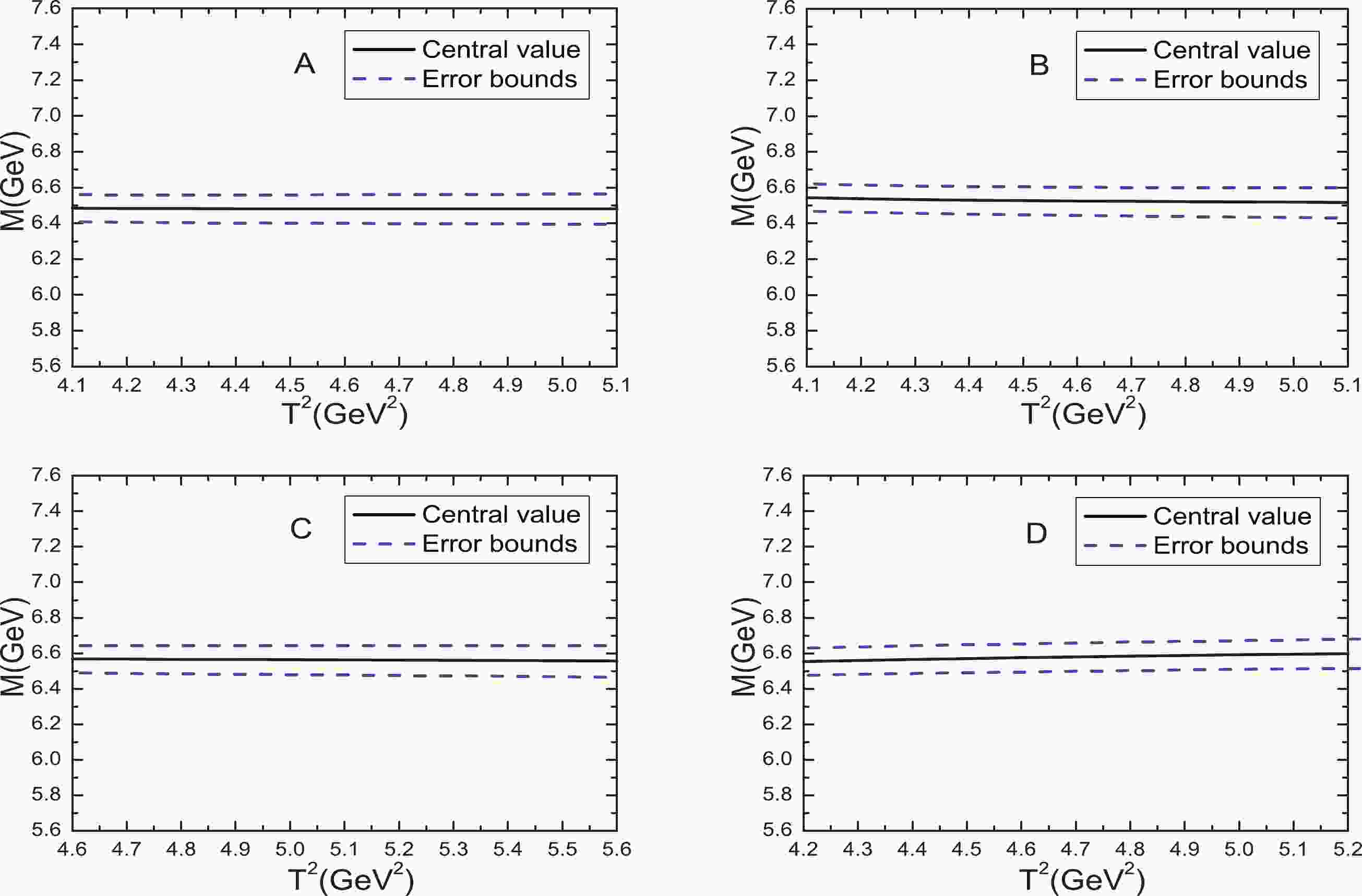
Now, let us take into account all uncertainties of the input parameters, and obtain the values of the masses and pole residues of the first radial excited states, which are also shown explicitly in Table 1 and Fig. 1. The predicted masses and pole residues are rather stable with variation of the Borel parameters; the uncertainties that originate from the Borel parameters in the Borel windows are very small, in other words, Borel platforms appear. Now that the three criteria are all satisfied, we expect to make reliable or sensible predictions.

Figure 1

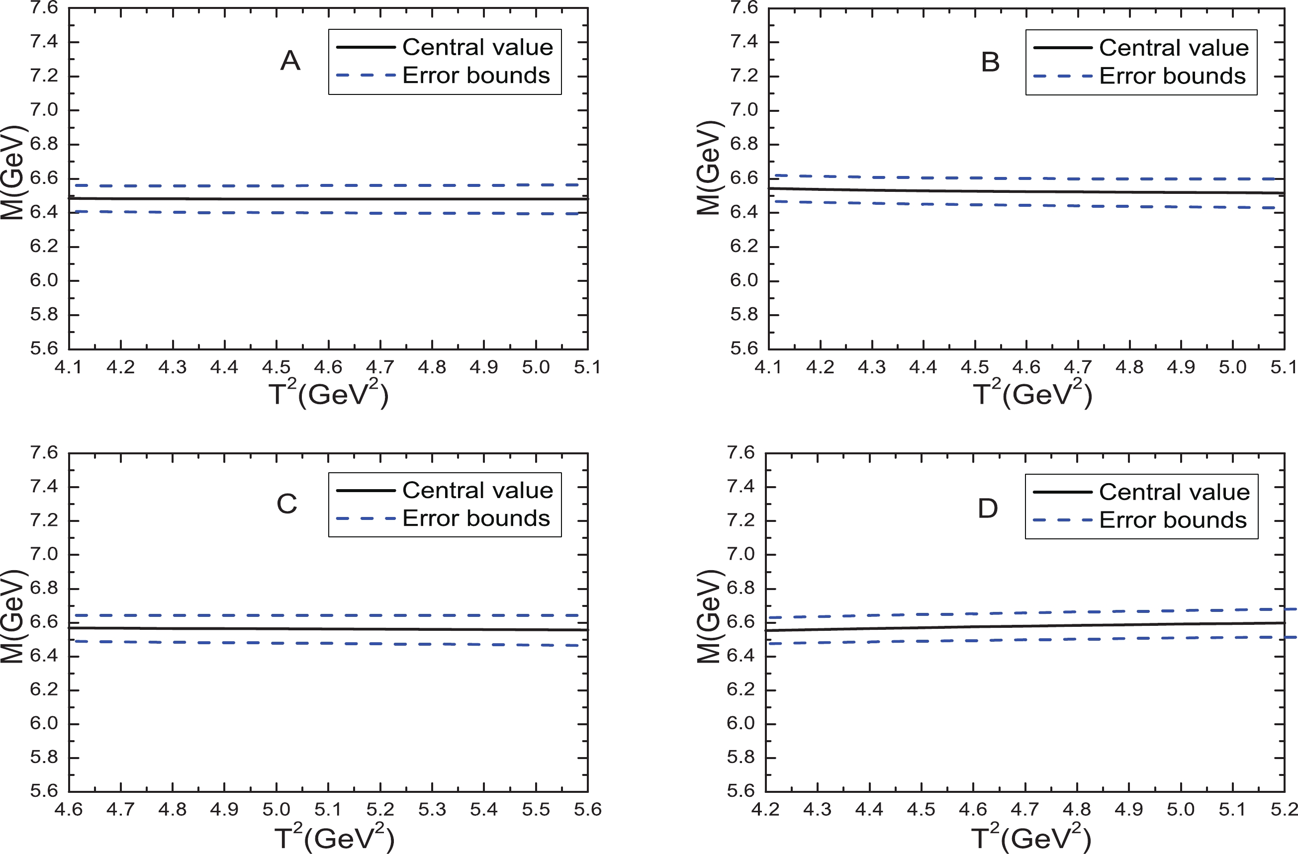
Figure 1. (color online) Masses of the first radial excited states of the tetraquark states with variations of the Borel parameters

$T^2$ , where A, B, C, and D denote the scalar, axialvector, vector, and tensor tetraquark states, respectively.

DownLoad: Full-Size Img PowerPoint

In Table 2, we present the masses of the ground states and the first radial excited states from the QCD sum rules [7, 8]. The masses of the ground states, the first radial excited states, the third radial excited states, etc., satisfy the Regge trajectories,

Table 2

Table 2. Masses of the

$cc\bar{c}\bar{c}$ tetraquark states with the radial quantum numbers

$n = 1$ ,

$2$ ,

$3$ , and

$4$ .

$J^{PC}$	$M_{1}/{\rm{GeV} }$ [7, 8]	$M_{2}/{\rm{GeV} }$	$M_{3}/{\rm{GeV} }$	$M_{ 4}/{\rm{GeV} }$
$0^{++}$	$5.99\pm0.08$	$6.48\pm0.08$	$6.94\pm0.08$	$7.36\pm0.08$
$1^{+-}$	$6.05\pm0.08$	$6.52\pm0.08$	$6.96\pm0.08$	$6.37\pm0.08$
$2^{++}$	$6.09\pm0.08$	$6.56\pm0.08$	$7.00\pm0.08$	$7.41\pm0.08$
$1^{--}$	$6.11\pm0.08$	$6.58\pm0.09$	$7.02\pm0.09$	$7.43\pm0.09$

DownLoad: CSV

Show Table

$M_n^2 = \alpha (n-1)+\alpha_0\, ,$

(30)

where $\alpha$ and $\alpha_0$ are constants. We take the masses of the ground states and the first radial excited states shown in Table 2 as input parameters to fit the parameters $\alpha$ and $\alpha_0$ , and obtain the masses of the second radial excited states, which are also shown in Table 2. From the Table, we can see that the mass gap $M_3-M_1 = 0.91\sim0.95\,{\rm{GeV}}$ , which is consistent with the mass gap $m_{\psi^{\prime\prime}}-m_{J/\psi} =$ 0.94 GeV. Furthermore, from Table 1, we can see that the continuum threshold parameters $\sqrt{s_0^\prime}\leqslant \overline{M}_3$ , where $\overline{M}_3$ represents the central values of the masses of the second radial excited states.

From Table 2, we can see that the predicted masses $M = 6.48\pm0.08\,{\rm{GeV}}$ , $6.52\pm0.08\,{\rm{GeV}}$ , $6.56\pm0.08\,{\rm{GeV}}$ , and $6.58\pm0.09\,{\rm{GeV}}$ for the first radial excited states of the scalar, axialvector, vector, and tensor $cc\bar{c}\bar{c}$ tetraquark states are consistent with the broad structure above the threshold ranging from 6.2 to 6.8 GeV in the di- $J/\psi$ mass spectrum [22, 23], while the predicted masses $M = 6.94\pm0.08\,{\rm{GeV}}$ and $6.96\pm0.08\,{\rm{GeV}}$ for the second radial excited states of the scalar and axialvector $cc\bar{c}\bar{c}$ tetraquark states are consistent with the narrow structure at approximately 6.9 GeV in the di- $J/\psi$ mass spectrum [22, 23]. The present predictions support assigning the broad structure from 6.2 to 6.8 GeV in the di- $J/\psi$ mass spectrum to be the first radial excited state of the scalar, axialvector, vector, or tensor $cc\bar{c}\bar{c}$ tetraquark state, and assigning the narrow structure at approximately 6.9 GeV in the di- $J/\psi$ mass spectrum to be the second radial excited state of the scalar or axialvector $cc\bar{c}\bar{c}$ tetraquark state.

In Table 2, we also present the third radial excited states of the $cc\bar{c}\bar{c}$ tetraquark states. From the Table, we can see that they lie above the vague structures near 7.2 GeV in the LHCb data [22, 23].

4. Conclusion

1. Introduction
2. QCD sum rules for the first radial excited ${{cc}\bar{ c}\bar{ c}}$ tetraquark states
3. Numerical results and discussion
4. Conclusion

In this article, we construct the scalar and tensor currents to study the first radial excited states of the scalar, axialvector, vector, and tensor diquark-antidiquark-type $cc\bar{c}\bar{c}$ tetraquark states with the QCD sum rules and obtain the masses and pole residues. Then, we use the Regge trajectories to obtain the masses of the second radial excited states. The present predictions support assigning the broad structure from 6.2 to 6.8 GeV in the di- $J/\psi$ mass spectrum to be the first radial excited state of the scalar, axialvector, vector, or tensor $cc\bar{c}\bar{c}$ tetraquark state, and assigning the narrow structure at approximately 6.9 GeV in the di- $J/\psi$ mass spectrum to be the second radial excited state of the scalar or axialvector $cc\bar{c}\bar{c}$ tetraquark state.

References

[1]	R. J. Lloyd and J. P. Vary, Phys. Rev. D, 70: 014009 (2004)
[2]	N. Barnea, J. Vijande, and A. Valcarce, Phys. Rev. D, 73: 054004 (2006)
[3]	A. V. Berezhnoy, A. V. Luchinsky, and A. A. Novoselov, Phys. Rev. D, 86: 034004 (2012)
[4]	W. Heupel, G. Eichmann, and C. S. Fischer, Phys. Lett. B, 718: 545 (2012)
[5]	Y. Bai, S. Lu, and J. Osborne, arXiv: 1612.00012
[6]	J. M. Richard, A. Valcarce, and J. Vijande, Phys. Rev. D, 95: 054019 (2017)
[7]	Z. G. Wang, Eur. Phys. J. C, 77: 432 (2017)
[8]	Z. G. Wang and Z. Y. Di, Acta Phys. Polon. B, 50: 1335 (2019)
[9]	M. Karliner, J. L. Rosner, and S. Nussinov, Phys. Rev. D, 95: 034011 (2017)
[10]	W. Chen, H. X. Chen, X. Liu et al., Phys. Lett. B, 773: 247 (2017)
[11]	M. N. Anwar, J. Ferretti, F. K. Guo et al., Eur. Phys. J. C, 78: 647 (2018)
[12]	A. Esposito and A. D. Polosa, Eur. Phys. J. C, 78: 782 (2018)
[13]	J. Wu, Y. R. Liu, K. Chen et al., Phys. Rev. D, 97: 094015 (2018)
[14]	C. Hughes, E. Eichten, and C. T. H. Davies, Phys. Rev. D, 97: 054505 (2018)
[15]	V. R. Debastiani and F. S. Navarra, Chin. Phys. C, 43: 013105 (2019)
[16]	M. S. Liu, Q. F. Lu, X. H. Zhong et al., Phys. Rev. D, 100: 016006 (2019)
[17]	X. Chen, arXiv: 2001.06755
[18]	M. A. Bedolla, J. Ferretti, C. D. Roberts et al., arXiv: 1911.00960
[19]	C. Deng, H. Chen, and J. Ping, arXiv: 2003.05154
[20]	P. Lundhammar and T. Ohlsson, arXiv: 2006.09393
[21]	M. S. liu, F. X. Liu, X. H. Zhong et al., arXiv: 2006.11952
[22]	Liupan An [On behalf of the LHCb Collaboration], Latest results on exotic hadrons at LHCb, https://indico.cern.ch/event/900972/
[23]	R. Aaij et al., arXiv: 2006.16957
[24]	M. A. Shifman, A. I. Vainshtein, and V. I. Zakharov, Nucl. Phys. B, 147: 385 (1979)
[25]	M. A. Shifman, A. I. Vainshtein, and V. I. Zakharov, Nucl. Phys. B, 147: 448 (1979)
[26]	L. J. Reinders, H. Rubinstein, and S. Yazaki, Phys. Rept., 127: 1 (1985) doi: 10.1016/0370-1573(85)90065-1
[27]	M. S. Maior de Sousa and R. Rodrigues da Silva, Braz. J. Phys., 46: 730 (2016) doi: 10.1007/s13538-016-0449-9
[28]	Z. G. Wang, Commun. Theor. Phys., 63: 325 (2015) doi: 10.1088/0253-6102/63/3/325
[29]	Z. G. Wang, Chin. Phys. C, 44: 063105 (2020)
[30]	P. Colangelo and A. Khodjamirian, hep-ph/0010175
[31]	M. Tanabashi et al., Phys. Rev. D, 98: 030001 (2018)

References

[1]	R. J. Lloyd and J. P. Vary, Phys. Rev. D, 70: 014009 (2004)
[2]	N. Barnea, J. Vijande, and A. Valcarce, Phys. Rev. D, 73: 054004 (2006)
[3]	A. V. Berezhnoy, A. V. Luchinsky, and A. A. Novoselov, Phys. Rev. D, 86: 034004 (2012)
[4]	W. Heupel, G. Eichmann, and C. S. Fischer, Phys. Lett. B, 718: 545 (2012)
[5]	Y. Bai, S. Lu, and J. Osborne, arXiv: 1612.00012
[6]	J. M. Richard, A. Valcarce, and J. Vijande, Phys. Rev. D, 95: 054019 (2017)
[7]	Z. G. Wang, Eur. Phys. J. C, 77: 432 (2017)
[8]	Z. G. Wang and Z. Y. Di, Acta Phys. Polon. B, 50: 1335 (2019)
[9]	M. Karliner, J. L. Rosner, and S. Nussinov, Phys. Rev. D, 95: 034011 (2017)
[10]	W. Chen, H. X. Chen, X. Liu et al., Phys. Lett. B, 773: 247 (2017)
[11]	M. N. Anwar, J. Ferretti, F. K. Guo et al., Eur. Phys. J. C, 78: 647 (2018)
[12]	A. Esposito and A. D. Polosa, Eur. Phys. J. C, 78: 782 (2018)
[13]	J. Wu, Y. R. Liu, K. Chen et al., Phys. Rev. D, 97: 094015 (2018)
[14]	C. Hughes, E. Eichten, and C. T. H. Davies, Phys. Rev. D, 97: 054505 (2018)
[15]	V. R. Debastiani and F. S. Navarra, Chin. Phys. C, 43: 013105 (2019)
[16]	M. S. Liu, Q. F. Lu, X. H. Zhong et al., Phys. Rev. D, 100: 016006 (2019)
[17]	X. Chen, arXiv: 2001.06755
[18]	M. A. Bedolla, J. Ferretti, C. D. Roberts et al., arXiv: 1911.00960
[19]	C. Deng, H. Chen, and J. Ping, arXiv: 2003.05154
[20]	P. Lundhammar and T. Ohlsson, arXiv: 2006.09393
[21]	M. S. liu, F. X. Liu, X. H. Zhong et al., arXiv: 2006.11952
[22]	Liupan An [On behalf of the LHCb Collaboration], Latest results on exotic hadrons at LHCb, https://indico.cern.ch/event/900972/
[23]	R. Aaij et al., arXiv: 2006.16957
[24]	M. A. Shifman, A. I. Vainshtein, and V. I. Zakharov, Nucl. Phys. B, 147: 385 (1979)
[25]	M. A. Shifman, A. I. Vainshtein, and V. I. Zakharov, Nucl. Phys. B, 147: 448 (1979)
[26]	L. J. Reinders, H. Rubinstein, and S. Yazaki, Phys. Rept., 127: 1 (1985) doi: 10.1016/0370-1573(85)90065-1
[27]	M. S. Maior de Sousa and R. Rodrigues da Silva, Braz. J. Phys., 46: 730 (2016) doi: 10.1007/s13538-016-0449-9
[28]	Z. G. Wang, Commun. Theor. Phys., 63: 325 (2015) doi: 10.1088/0253-6102/63/3/325
[29]	Z. G. Wang, Chin. Phys. C, 44: 063105 (2020)
[30]	P. Colangelo and A. Khodjamirian, hep-ph/0010175
[31]	M. Tanabashi et al., Phys. Rev. D, 98: 030001 (2018)

[1]	Xiao-Song Yang , Zhi-Gang Wang . Strong decays of the fully-charm tetraquark states with explicit P-waves via the QCD sum rules. Chinese Physics C, 2025, 49(7): 1-10.
[2]	Xiu-Wu Wang , Zhi-Gang Wang . Strong decays of the P_c(4312) and its isospin cousin via the QCD sum rules. Chinese Physics C, 2024, 48(5): 053102. doi: 10.1088/1674-1137/ad2442
[3]	Zhi-Gang Wang . B_c meson and its scalar cousin with QCD sum rules. Chinese Physics C, 2024, 48(10): 103104. doi: 10.1088/1674-1137/ad5a71
[4]	Zhi-Gang Wang . Ground states and first radial excitations of vector tetraquark states with explicit P-waves via QCD sum rules. Chinese Physics C, 2024, 48(10): 103103. doi: 10.1088/1674-1137/ad5ae5
[5]	Bing-Dong Wan , Hong-Tai Xu . 0^{– –} hidden-heavy tetraquark states via QCD sum rules. Chinese Physics C, 2024, 48(9): 093103. doi: 10.1088/1674-1137/ad53b7
[6]	Ze-Sheng Chen , Zhuo-Ran Huang , Hong-Ying Jin , T.G. Steele , Zhu-Feng Zhang . Mixing of X and Y states from QCD sum rules analysis. Chinese Physics C, 2022, 46(6): 063102. doi: 10.1088/1674-1137/ac531a
[7]	Ren-Hua Wu , Yu-Sheng Zuo , Ce Meng , Yan-Qing Ma , Kuang-Ta Chao . NLO effects for Ω_QQQ baryons in QCD Sum Rules. Chinese Physics C, 2021, 45(9): 093103. doi: 10.1088/1674-1137/ac0b3c
[8]	Zhi-Gang Wang , Hui-Juan Wang . Analysis of the 1S and 2S states of Λ_Q and Ξ_Q with QCD sum rules. Chinese Physics C, 2021, 45(1): 013109. doi: 10.1088/1674-1137/abc1d3
[9]	Zhi-Gang Wang , Qi Xin . Analysis of hidden-charm pentaquark molecular states with and without strangeness via the QCD sum rules. Chinese Physics C, 2021, 45(12): 123105. doi: 10.1088/1674-1137/ac2a1d
[10]	Zhi-Gang Wang , Xu Wang . Analysis of the strong decays of P_c(4312) as a pentaquark molecular state with QCD sum rules. Chinese Physics C, 2020, 44(10): 103102. doi: 10.1088/1674-1137/ababf7
[11]	Jia-Bing Xiang , Hua-Xing Chen , Wei Chen , Xiao-Bo Li , Xing-Qun Yao , Shi-Lin Zhu . Revisiting hidden-charm pentaquarks from QCD sum rules. Chinese Physics C, 2019, 43(3): 034104. doi: 10.1088/1674-1137/43/3/034104
[12]	Xiao-Hui Hu , Yue-Long Shen , Wei Wang , Zhen-Xing Zhao . Weak decays of doubly heavy baryons: “decay constants”. Chinese Physics C, 2018, 42(12): 123102. doi: 10.1088/1674-1137/42/12/123102
[13]	Guo-Liang Yu , Zhi-Gang Wang , Zhen-Yu Li . Analysis of the strong coupling form factors of ∑_bNB and∑_cND in QCD sum rules. Chinese Physics C, 2017, 41(8): 083104. doi: 10.1088/1674-1137/41/8/083104
[14]	Qi-Nan Wang , Zhu-Feng Zhang , T. G. Steele , Hong-Ying Jin , Zhuo-Ran Huang . A comprehensive revisit of the ρ meson with improved Monte-Carlo based QCD sum rules. Chinese Physics C, 2017, 41(7): 074107. doi: 10.1088/1674-1137/41/7/074107
[15]	SUN Yan-Jun , WANG Zhi-Gang , HUANG Tao . B → A transitions in the light-cone QCD sum rules with the chiral current. Chinese Physics C, 2012, 36(11): 1046-1054. doi: 10.1088/1674-1137/36/11/003
[16]	LI Jing-Wu , XUE Dan-Qing , XU Qing-Qiang , WU Xiang-Yao . D⁺ → η^(')l⁺ν_l semileptonic decays in light-cone sum rules. Chinese Physics C, 2011, 35(6): 519-524. doi: 10.1088/1674-1137/35/6/001
[17]	ZHANG Jian-Rong , HUANG Ming-Qiu . Heavy flavor baryon spectra via QCD sum rules. Chinese Physics C, 2009, 33(12): 1385-1388. doi: 10.1088/1674-1137/33/12/061
[18]	ZHANG Ai-Lin . Light four-quark states and QCD sum rule. Chinese Physics C, 2009, 33(6): 494-496. doi: 10.1088/1674-1137/33/6/017
[19]	Lu Wentao , Liu Jueping . Quantum Chromodynamics Sum Rules for the 0⁺⁺ Three-Gluon Scalar Glueball. Chinese Physics C, 1996, 20(S3): 261-268.
[20]	Ding Yibing , Zhou Lei , Zhao Guangda , Qin Danhua . Sum Rules in Quantum Mechanics and the Electric Dipole Transitions of the ψ (3770). Chinese Physics C, 1991, 15(S4): 373-383.

Access

Cited by

1.	Bai, X.-W., Huang, Y., Sang, W.-L. Light quark fragmentation into an S-wave fully charmed tetraquark[J]. Physical Review D, 2025, 111(5): 054006. doi: 10.1103/PhysRevD.111.054006
2.	Liu, W.-Y., Chen, H.-X. Hadronic Molecules with Four Charm or Beauty Quarks[J]. Universe, 2025, 11(2): 36. doi: 10.3390/universe11020036
3.	Wang, Z.-G., Yang, X.-S. The two-body strong decays of the fully-charm tetraquark states[J]. AAPPS Bulletin, 2024, 34(1): 5. doi: 10.1007/s43673-023-00112-4
4.	Zhang, H.-F., Mo, X.-M., Yan, Y.-P. Hadronic decay of exotic mesons consisting of four charm quarks[J]. Physical Review D, 2024, 110(9): 096021. doi: 10.1103/PhysRevD.110.096021
5.	Mistry, R., Majethiya, A. Spectroscopic study of exotic fully-heavy tetraquark states QQQ̄Q̄ (Q∈c,b)[J]. Chinese Journal of Physics, 2024. doi: 10.1016/j.cjph.2024.08.040
6.	Feng, F., Huang, Y., Jia, Y. et al. Photoproduction of fully charmed tetraquark at electron-ion colliders[J]. Physical Review D, 2024, 110(5): 054007. doi: 10.1103/PhysRevD.110.054007
7.	Bai, X.-W., Feng, F., Gan, C.-M. et al. Producing fully-charmed tetraquarks via charm quark fragmentation in colliders[J]. Journal of High Energy Physics, 2024, 2024(9): 2. doi: 10.1007/JHEP09(2024)002
8.	Lin, Y.-Y., Wang, J.-Y., Zhang, A. Mass spectrum of fully charmed [cc][c¯c¯] tetraquarks[J]. European Physical Journal Plus, 2024, 139(8): 707. doi: 10.1140/epjp/s13360-024-05480-w
9.	Tang, C.-M., Duan, C.-G., Tang, L. Fully charmed tetraquark states in 8[cc¯]⊗8[cc¯] color structure via QCD sum rules[J]. European Physical Journal C, 2024, 84(7): 743. doi: 10.1140/epjc/s10052-024-13102-z
10.	Chen, Z.-Z., Chen, X.-L., Yang, P.-F. et al. P -wave fully charm and fully bottom tetraquark states[J]. Physical Review D, 2024, 109(9): 094011. doi: 10.1103/PhysRevD.109.094011
11.	Liu, M.-S., Liu, F.-X., Zhong, X.-H. et al. Fully heavy tetraquark states and their evidences in LHC observations[J]. Physical Review D, 2024, 109(7): 076017. doi: 10.1103/PhysRevD.109.076017
12.	Sang, W.-L., Wang, T., Zhang, Y.-D. et al. Electromagnetic and hadronic decay of fully heavy tetraquarks[J]. Physical Review D, 2024, 109(5): 056016. doi: 10.1103/PhysRevD.109.056016
13.	Ortega, P.G., Entem, D.R., Fernández, F. Exploring Tψψ tetraquark candidates in a coupled-channels formalism[J]. Physical Review D, 2023, 108(9): 094023. doi: 10.1103/PhysRevD.108.094023
14.	Agaev, S.S., Azizi, K., Barsbay, B. et al. Exploring fully heavy scalar tetraquarks QQQ‾Q‾[J]. Physics Letters, Section B: Nuclear, Elementary Particle and High-Energy Physics, 2023. doi: 10.1016/j.physletb.2023.138089
15.	Feng, F., Huang, Y., Jia, Y. et al. Inclusive production of fully charmed tetraquarks at the LHC[J]. Physical Review D, 2023, 108(5): L051501. doi: 10.1103/PhysRevD.108.L051501
16.	Li, Q., Chang, C.-H., Wang, T. et al. Strong decays of PψN(4312)+ to J/ψ(ηc)p and D¯ (∗)Λ c within the Bethe-Salpeter framework[J]. Journal of High Energy Physics, 2023, 2023(6): 189. doi: 10.1007/JHEP06(2023)189
17.	Dong, W.-C., Wang, Z.-G. Going in quest of potential tetraquark interpretations for the newly observed Tψψ states in light of the diquark-antidiquark scenarios[J]. Physical Review D, 2023, 107(7): 074010. doi: 10.1103/PhysRevD.107.074010
18.	Chen, H.-X., Chen, W., Liu, X. et al. An updated review of the new hadron states[J]. Reports on Progress in Physics, 2023, 86(2): 026201. doi: 10.1088/1361-6633/aca3b6
19.	Feng, F., Huang, Y., Jia, Y. et al. Fragmentation production of fully-charmed tetraquarks at the LHC[J]. Physical Review D, 2022, 106(11): 114029. doi: 10.1103/PhysRevD.106.114029
20.	Faustov, R.N., Galkin, V.O., Savchenko, E.M. Fully Heavy Tetraquark Spectroscopy in the Relativistic Quark Model[J]. Symmetry, 2022, 14(12): 2504. doi: 10.3390/sym14122504
21.	Wang, Z.-G.. Analysis of the X(6600), X(6900), X(7300) and related tetraquark states with the QCD sum rules[J]. Nuclear Physics B, 2022. doi: 10.1016/j.nuclphysb.2022.115983
22.	Mutuk, H.. Spectrum of ccb¯b¯, bcc¯c¯, and bcb¯b¯ tetraquark states in the dynamical diquark model[J]. Physics Letters, Section B: Nuclear, Elementary Particle and High-Energy Physics, 2022. doi: 10.1016/j.physletb.2022.137404
23.	Chen, H.-X., Yan, Y.-X., Chen, W. Decay behaviors of the fully bottom and fully charm tetraquark states[J]. Physical Review D, 2022, 106(9): 094019. doi: 10.1103/PhysRevD.106.094019
24.	Chen, W., Wang, Q.-N., Yang, Z.-Y. et al. Searching for fully-heavy tetraquark states in QCD moment sum rules[J]. Nuclear and Particle Physics Proceedings, 2022. doi: 10.1016/j.nuclphysbps.2022.09.016
25.	Wu, R.-H., Zuo, Y.-S., Wang, C.-Y. et al. NLO results with operator mixing for fully heavy tetraquarks in QCD sum rules[J]. Journal of High Energy Physics, 2022, 2022(11): 23. doi: 10.1007/JHEP11(2022)023
26.	Wang, Z.-G.. Fully heavy hexaquark states via the QCD sum rules[J]. International Journal of Modern Physics A, 2022, 37(26): 2250166. doi: 10.1142/S0217751X22501664
27.	Wang, J.-Z., Liu, X. Improved understanding of the peaking phenomenon existing in the new di- J/ψ invariant mass spectrum from the CMS Collaboration[J]. Physical Review D, 2022, 106(5): 054015. doi: 10.1103/PhysRevD.106.054015
28.	Wang, Z.-G., Xin, Q. Analysis of the bottom-charm baryon states with QCD sum rules[J]. International Journal of Modern Physics A, 2022, 37(11-12): 2250074. doi: 10.1142/S0217751X22500749
29.	Zhuang, Z., Zhang, Y., Ma, Y. et al. Lineshape of the compact fully heavy tetraquark[J]. Physical Review D, 2022, 105(5): 054026. doi: 10.1103/PhysRevD.105.054026
30.	Yan, Y., Wu, Y., Hu, X. et al. Fully heavy pentaquarks in quark models[J]. Physical Review D, 2022, 105(1): 014027. doi: 10.1103/PhysRevD.105.014027
31.	Dong, X.-K., Baru, V., Guo, F.-K. et al. Is the existence of a J/ψJ/ψ bound state plausible?[J]. Science Bulletin, 2021, 66(24): 2462-2470. doi: 10.1016/j.scib.2021.09.009
32.	Wang, Z.-G.. Analysis of the triply heavy baryon states with the QCD sum rules[J]. AAPPS Bulletin, 2021, 31(1): 5. doi: 10.1007/s43673-021-00006-3
33.	Wang, Q.-N., Yang, Z.-Y., Chen, W. Exotic fully heavy Q Q ¯ Q Q ¯ tetraquark states in 8 [Q Q ¯]- 8 [Q Q ¯] color configuration EXOTIC FULLY HEAVY Q Q ¯ Q Q ¯ ⋯ WANG QI-NAN, YANG ZI-YAN, and CHEN WEI[J]. Physical Review D, 2021, 104(11): 114037. doi: 10.1103/PhysRevD.104.114037
34.	Liu, F.-X., Liu, M.-S., Zhong, X.-H. et al. Higher mass spectra of the fully-charmed and fully-bottom tetraquarks[J]. Physical Review D, 2021, 104(11): 116029. doi: 10.1103/PhysRevD.104.116029
35.	Lü, Q.-F., Chen, D.-Y., Dong, Y.-B. et al. Triply-heavy tetraquarks in an extended relativized quark model[J]. Physical Review D, 2021, 104(5): 054026. doi: 10.1103/PhysRevD.104.054026
36.	Liang, Z.-R., Wu, X.-Y., Yao, D.-L. Hunting for states in the recent LHCb di- J /ψ invariant mass spectrum[J]. Physical Review D, 2021, 104(3): 034034. doi: 10.1103/PhysRevD.104.034034
37.	Nefediev, A.V.. X(6200) as a compact tetraquark in the QCD string model[J]. European Physical Journal C, 2021, 81(8): 692. doi: 10.1140/epjc/s10052-021-09511-z
38.	Wang, Q.-N., Yang, Z.-Y., Chen, W. et al. Mass spectra for the and tetraquark states[J]. Physical Review D, 2021, 104(1): 014020. doi: 10.1103/PhysRevD.104.014020
39.	Li, Q., Chang, C.-H., Wang, G.-L. et al. Mass spectra and wave functions of tetraquarks[J]. Physical Review D, 2021, 104(1): 014018. doi: 10.1103/PhysRevD.104.014018
40.	Yang, G., Ping, J., Segovia, J. Exotic resonances of fully-heavy tetraquarks in a lattice-QCD insipired quark model[J]. Physical Review D, 2021, 104(1): 014006. doi: 10.1103/PhysRevD.104.014006
41.	Wan, B.-D., Qiao, C.-F. Gluonic tetracharm configuration of X(6900)[J]. Physics Letters, Section B: Nuclear, Elementary Particle and High-Energy Physics, 2021. doi: 10.1016/j.physletb.2021.136339
42.	Gonçalves, V.P., Moreira, B.D. Fully - heavy tetraquark production by γγ interactions in hadronic collisions at the LHC[J]. Physics Letters, Section B: Nuclear, Elementary Particle and High-Energy Physics, 2021. doi: 10.1016/j.physletb.2021.136249
43.	Wang, J.-Z., Liu, X., Matsuki, T. Fully-heavy structures in the invariant mass spectrum of J/ψψ(3686), J/ψψ(3770), ψ(3686)ψ(3686), and J/ψϒ(1S) at hadron colliders[J]. Physics Letters, Section B: Nuclear, Elementary Particle and High-Energy Physics, 2021. doi: 10.1016/j.physletb.2021.136209
44.	Zhukova, V.I., Nefediev, A.V., Pakhlov, P.N. et al. Super-factory of bottomed hadrons Belle II[J]. Physics-Uspekhi, 2021, 64(5): 468-494. doi: 10.3367/UFNe.2020.10.038847
45.	Ke, H.-W., Han, X., Liu, X.-H. et al. Tetraquark state X(6900) and the interaction between diquark and antidiquark[J]. European Physical Journal C, 2021, 81(5): 427. doi: 10.1140/epjc/s10052-021-09229-y
46.	Wang, J.-Z., Chen, D.-Y., Liu, X. et al. Producing fully charm structures in the J /ψ -pair invariant mass spectrum[J]. Physical Review D, 2021, 103(7): L071503. doi: 10.1103/PhysRevD.103.L071503
47.	Dong, X.-K., Baru, V., Guo, F.-K. et al. Coupled-Channel Interpretation of the LHCb Double- J /ψ Spectrum and Hints of a New State near the J /ψJ /ψ Threshold[J]. Physical Review Letters, 2021, 126(13): 132001. doi: 10.1103/PhysRevLett.126.132001
48.	Guo, Z.-H., Oller, J.A. Insights into the inner structures of the fully charmed tetraquark state X (6900)[J]. Physical Review D, 2021, 103(3): 034024. doi: 10.1103/PhysRevD.103.034024
49.	Liu, F.-X., Liu, M.-S., Zhong, X.-H. et al. Fully strange tetraquark ss s ¯ s ¯ spectrum and possible experimental evidence FULLY-STRANGE TETRAQUARK SS S ¯ S ¯ ... FENG-XIAO LIU et al.[J]. Physical Review D, 2021, 103(1): 016016. doi: 10.1103/PhysRevD.103.016016
50.	Wang, Z.-G.. Revisit the tetraquark candidates in the J/ψ J/ψ mass spectrum[J]. International Journal of Modern Physics A, 2021, 36(2): 2150014. doi: 10.1142/S0217751X21500147
51.	Zhang, J.-R.. 0+ fully-charmed tetraquark states[J]. Physical Review D, 2021, 103(1): 014018. doi: 10.1103/PhysRevD.103.014018
52.	Maciuła, R., Schäfer, W., Szczurek, A. On the mechanism of T4c(6900) tetraquark production[J]. Physics Letters, Section B: Nuclear, Elementary Particle and High-Energy Physics, 2021. doi: 10.1016/j.physletb.2020.136010
53.	Karliner, M., Rosner, J.L. Interpretation of structure in the di- J /ψ spectrum[J]. Physical Review D, 2020, 102(11): 114039. doi: 10.1103/PhysRevD.102.114039
54.	Wang, X.-Y., Lin, Q.-Y., Xu, H. et al. Discovery potential for the LHCb fully charm tetraquark X (6900) state via p ¯ p annihilation reaction DISCOVERY POTENTIAL for the LHCB FULLY-CHARM ... WANG, LIN, XU, XIE, HUANG, and CHEN[J]. Physical Review D, 2020, 102(11): 116014. doi: 10.1103/PhysRevD.102.116014
55.	Yang, G., Ping, J., Segovia, J. Tetra-and penta-quark structures in the constituent quark model[J]. Symmetry, 2020, 12(11): 1-79. doi: 10.3390/sym12111869

Figures(1) / Tables(2)

Get Citation

Zhi-Gang Wang. Tetraquark candidates in the LHCb's di-J/ψ mass spectrum[J]. Chinese Physics C. doi: 10.1088/1674-1137/abb080

Zhi-Gang Wang. Tetraquark candidates in the LHCb's di-J/ψ mass spectrum[J]. Chinese Physics C. doi: 10.1088/1674-1137/abb080 shu

RIS(for EndNote,Reference Manager,ProCite)

BibTex

Txt

Milestone

Received: 2020-06-24

Article Metric

Article Views(1997)
PDF Downloads(45)
Cited by(55)

Policy on re-use

To reuse of subscription content published by CPC, the users need to request permission from CPC, unless the content was published under an Open Access license which automatically permits that type of reuse.

通讯作者: 陈斌, bchen63@163.com

1.
沈阳化工大学材料科学与工程学院沈阳 110142

HTML

1. Introduction

The charmonium-like and bottomonium-like states are good subjects for studying exotic states and understanding strong interactions. If they are genuine tetraquark states, there are two heavy valence quarks and two light valence quarks; therefore, the dynamics is complex compared with that of tetraquark configurations, which consist of four heavy valence quarks. The attractive interactions between the two heavy quarks (or antiquarks) should dominate over short distances and favor the formation of genuine diquark-antidiquark-type tetraquark states, rather than the loosely bound tetraquark molecular states, because the light mesons cannot be exchanged between the two heavy quarkonia to provide attraction at the leading order. In recent years, the full-heavy tetraquark states have attracted much attention and have been studied extensively [1-21].

Recently, the LHCb collaboration reported their preliminary results on the observations of $cc\bar{c}\bar{c}$ tetraquark candidates in the di- $J/\psi$ invariant mass spectrum at $p_T> 5.2\,{\rm{GeV}}$ [22, 23]. They observed a broad structure above the threshold ranging from 6.2 to 6.8 GeV and a narrow structure at approximately 6.9 GeV with a significance of greater than $5\sigma$ ; they also observed some vague structures near 7.2 GeV. The masses of the full-heavy tetraquark states from the phenomenological quark models lie either above or below the di- $J/\psi$ or di- $\Upsilon$ threshold, and vary over a large range [1-21]. This is the first time that clear structures in the di- $J/\psi$ mass spectrum have been observed experimentally and may be evidence for genuine $cc\bar{c}\bar{c}$ tetraquark states. The observation of evidence for the $cc\bar{c}\bar{c}$ tetraquark states provides important experimental constraints on the theoretical models, sheds light on the nature of the exotic states, and plays an important role in establishing the tetraquark states.

In Refs. [7, 8], we study the mass spectrum of the ground states of the scalar, axialvector, vector, and tensor full-heavy diquark-antidiquark-type tetraquark states with the QCD sum rules, showing that the predicted tetraquark masses lie blow the di- $J/\psi$ or di- $\Upsilon$ threshold. In the present work, we extend our previous work to study the mass spectrum of the first radial excited states of the scalar, axialvector, vector, and tensor diquark-antidiquark-type $cc\bar{c}\bar{c}$ tetraquark states with the QCD sum rules; then, we take the masses of the ground states and the first radial excited states as the input parameters, resort to the Regge trajectories to obtain the masses of the second radial excited states, and make possible assignments of LHCb's new structures.

The article is arranged as follows: we derive the QCD sum rules for the masses and pole residues of the first radial excited states of the $cc\bar{c}\bar{c}$ tetraquark states in Sec. 2; in Sec. 3, we present the numerical results and use the Regge trajectories to obtain the masses of the second radial excited states; Sec. 4 is reserved for our conclusions.

2. QCD sum rules for the first radial excited ${{cc}\bar{ c}\bar{ c}}$ tetraquark states

4. Conclusion

In this article, we construct the scalar and tensor currents to study the first radial excited states of the scalar, axialvector, vector, and tensor diquark-antidiquark-type $cc\bar{c}\bar{c}$ tetraquark states with the QCD sum rules and obtain the masses and pole residues. Then, we use the Regge trajectories to obtain the masses of the second radial excited states. The present predictions support assigning the broad structure from 6.2 to 6.8 GeV in the di- $J/\psi$ mass spectrum to be the first radial excited state of the scalar, axialvector, vector, or tensor $cc\bar{c}\bar{c}$ tetraquark state, and assigning the narrow structure at approximately 6.9 GeV in the di- $J/\psi$ mass spectrum to be the second radial excited state of the scalar or axialvector $cc\bar{c}\bar{c}$ tetraquark state.

Reference (31)

Tetraquark candidates in LHCb's di-J/ψ mass spectrum

Abstract：

1. Introduction

1. Introduction
2. QCD sum rules for the first radial excited ${{cc}\bar{ c}\bar{ c}}$ tetraquark states
3. Numerical results and discussion
4. Conclusion

2. QCD sum rules for the first radial excited ${{cc}\bar{ c}\bar{ c}}$ tetraquark states

1. Introduction
2. QCD sum rules for the first radial excited ${{cc}\bar{ c}\bar{ c}}$ tetraquark states
3. Numerical results and discussion
4. Conclusion

3. Numerical results and discussion

1. Introduction
2. QCD sum rules for the first radial excited ${{cc}\bar{ c}\bar{ c}}$ tetraquark states
3. Numerical results and discussion
4. Conclusion

Table 1

Figure 1

Table 2

4. Conclusion

1. Introduction
2. QCD sum rules for the first radial excited ${{cc}\bar{ c}\bar{ c}}$ tetraquark states
3. Numerical results and discussion
4. Conclusion

References

References

Access

Cited by

Article Metrics

Metrics

通讯作者: 陈斌, bchen63@163.com

Email This Article

Tetraquark candidates in LHCb's di-J/ψ mass spectrum

Corresponding author: Zhi-Gang Wang, zgwang@aliyun.com

HTML

目录

Tetraquark candidates in LHCb's di-J/ψ mass spectrum

Abstract：

1. Introduction 1. Introduction 2. QCD sum rules for the first radial excited ccˉcˉc {{cc}\bar{ c}\bar{ c}} tetraquark states 3. Numerical results and discussion 4. Conclusion

2. QCD sum rules for the first radial excited ccˉcˉc {{cc}\bar{ c}\bar{ c}} tetraquark states 1. Introduction 2. QCD sum rules for the first radial excited ccˉcˉc {{cc}\bar{ c}\bar{ c}} tetraquark states 3. Numerical results and discussion 4. Conclusion

3. Numerical results and discussion 1. Introduction 2. QCD sum rules for the first radial excited ccˉcˉc {{cc}\bar{ c}\bar{ c}} tetraquark states 3. Numerical results and discussion 4. Conclusion

Table 1

Figure 1

Table 2

4. Conclusion 1. Introduction 2. QCD sum rules for the first radial excited ccˉcˉc {{cc}\bar{ c}\bar{ c}} tetraquark states 3. Numerical results and discussion 4. Conclusion

References

References

Access

Cited by

Article Metrics

Metrics

通讯作者: 陈斌, bchen63@163.com

Email This Article

Tetraquark candidates in LHCb's di-J/ψ mass spectrum

Corresponding author: Zhi-Gang Wang, zgwang@aliyun.com

HTML

目录

1. Introduction

1. Introduction
2. QCD sum rules for the first radial excited ${{cc}\bar{ c}\bar{ c}}$ tetraquark states
3. Numerical results and discussion
4. Conclusion

2. QCD sum rules for the first radial excited ${{cc}\bar{ c}\bar{ c}}$ tetraquark states

1. Introduction
2. QCD sum rules for the first radial excited ${{cc}\bar{ c}\bar{ c}}$ tetraquark states
3. Numerical results and discussion
4. Conclusion

3. Numerical results and discussion

1. Introduction
2. QCD sum rules for the first radial excited ${{cc}\bar{ c}\bar{ c}}$ tetraquark states
3. Numerical results and discussion
4. Conclusion

4. Conclusion

1. Introduction
2. QCD sum rules for the first radial excited ${{cc}\bar{ c}\bar{ c}}$ tetraquark states
3. Numerical results and discussion
4. Conclusion