


 Abstract
 HTML
HTML Reference
 Related
 PDF
PDF


-
Very recently, the BESIII Collaboration announced a new structure near the
$ D_{s}^{-} D^{* 0} $ and$ D_{s}^{*-} D^{0} $ thresholds in the$ K^+ $ recoil-mass spectra in$ e^{+} e^{-} \rightarrow K^{+}\left(D_{s}^{-} D^{* 0}+D_{s}^{*-} D^{0}\right) $ [1]. The pole mass and width of this$ Z_{cs}(3985)^- $ resonance were measured as$ \left(3982.5_{-2.6}^{+1.8} \pm 2.1\right) {\rm{MeV}} $ and$ \left(12.8_{-4.4}^{+5.3} \pm 3.0\right) {\rm{MeV}} $ , respectively. Decaying into$ D_{s}^{-} D^{* 0} $ and$ D_{s}^{*-} D^{0} $ in the S-wave, the spin-parity of$ Z_{cs}(3985)^- $ is assumed to favor$ J^P = 1^+ $ and the quark content$ c\bar cs\bar u $ [1]. It will be the first candidate for the hidden-charm four-quark state with strangeness.In previous theoretical investigations of the hidden-charm four-quark states with strangeness, the compact tetraquark configuration
$ sc\bar{q}\bar{c} $ has been studied in the color-magnetic interaction method [2] and QCD sum rules [3-10]. In Ref. [11], the authors investigated charged charmonium-like structures with hidden-charm and open-strange channels using the initial single chiral particle emission mechanism. Their results suggested the existence of enhancement structures near the thresholds of$ \bar{D}^{(*)}D_{s}^{(*)} $ . In Ref. [12], an axial-vector hidden-charm$ D^{*-} D_{s}^{+}-D^{-} D_{s}^{*+} $ molecular state was also predicted to exist. Possible$ D\bar{D}_{s0}^{*}(2317) $ and$ D^{*}\bar{D}_{s1}^{*}(2460) $ molecules were studied in Ref. [13], in which the results disfavor the existence of such states.A hadronic molecule is composed of two color-singlet hadrons by exchanging light mesons. This is a very useful configuration to study the nature of some exotic XYZ states and pentaquark states [14-19]. Because
$ Z_{cs}(3985)^- $ lies very close to the mass thresholds of$ D_{s}^{-} D^{* 0} $ and$ D_{s}^{*-} D^{0} $ , it is naturally studied in a molecular picture [20-27], as a partner state of$ Z_c(3900) $ discovered by BESIII [28]. It is also explained as a compound mixture of four different four-quark configurations [29], or a reflection structure of the charmed-strange meson$ D_{s2}^\ast(2573) $ [30]. In addition, the production mechanisms of the hidden-charm four-quark states with strangeness have been studied in Refs. [31, 32]. In Ref. [4], the authors studied the decay width of the$ D_s\bar D^\ast/D_s^\ast\bar D $ by calculating the three-point correlation functions in QCD sum rules. Their result for the total width suffers from a large uncertainty, although its central value is consistent with the experimental result of$ Z_{cs}(3985)^- $ . Such large uncertainty for the total width originates from the square of the form factors, which is inherent and difficult to be reduced using the method of three-point QCD sum rules. We also refer to the works [33-39] for recent studies on$ Z_{cs}(3985) $ using other methods. In this work, we shall study the exotic$ \bar{D}_s^{(*)}D^{(*)} $ molecular states and$ sc\bar q\bar c $ tetraquark states with$ J^P = 0^+, 1^+, 2^+ $ using the method of QCD sum rules [40-42].The paper is organized as follows. In Sec. II, we construct the interpolating currents for the
$ \bar{D}_s^{(*)}D^{(*)} $ molecular systems and$ sc\bar q\bar c $ tetraquark systems with$ J^{P} = 0^{+},1^{+} $ , and$ 2^{+} $ . In Sec. III, we calculate the correlation functions and spectral densities for these interpolating currents. We extract the masses for the$ \bar{D}_s^{(*)}D^{(*)} $ molecular states and$ sc\bar q\bar c $ tetraquark states by performing the QCD sum rule analyses in Sec. IV. The last section presents a summary and discussion. -
The color structures of a molecular field
$ [q \bar{Q}][Q \bar{q}] $ and a tetraquark field$ [q Q][\bar Q \bar{q}] $ can be written via the SU(3) symmetry,$\begin{aligned}[b] (\mathbf{3} \!\otimes\! \overline{\mathbf{3}})_{[q \bar{Q}]} \!\otimes\!(\mathbf{3} \!\otimes\! \overline{\mathbf{3}})_{[Q \bar{q}]} & = \!(\mathbf{1} \!\oplus\! \mathbf{8})_{[q \bar{Q}]} \!\otimes\!(\mathbf{1} \!\oplus\! \mathbf{8})_{[Q \bar{q}]} \\ &=\! (\mathbf{1} \!\otimes\! \mathbf{1}) \!\oplus\!(\mathbf{1} \!\otimes\! \mathbf{8}) \!\oplus\!(\mathbf{8} \!\otimes\! \mathbf{1}) \!\oplus\!(\mathbf{8} \!\otimes\! \mathbf{8}) \\ &=\! \mathbf{1} \!\oplus\! \mathbf{8} \!\oplus\! \mathbf{8} \!\oplus\!(\mathbf{1} \!\oplus\! \mathbf{8} \!\oplus\! \mathbf{8} \!\oplus\! \mathbf{1 0} \!\oplus\! \overline{\mathbf{1 0}} \!\oplus\! \mathbf{27})\, ,\\ (\mathbf{3} \!\otimes\! {\mathbf{3}})_{[q Q]} \!\otimes\!(\overline{\mathbf{3}} \!\otimes\! \overline{\mathbf{3}})_{[\bar Q \bar{q}]} &=\! (\mathbf{6} \!\oplus\! \overline{\mathbf{3}})_{[q Q]} \!\otimes\!(\mathbf{3} \!\oplus\! \overline{\mathbf{6}})_{[\bar Q \bar{q}]} \\ &=\! (\mathbf{6} \!\otimes\! \overline{\mathbf{6}}) \!\oplus\!(\overline{\mathbf{3}} \!\otimes\! \mathbf{3}) \!\oplus\! (\mathbf{6} \!\otimes\! \mathbf{3}) \!\oplus\!(\overline{\mathbf{3}} \!\otimes\! \overline{\mathbf{6}}) \\ &=\! (\mathbf{1} \!\oplus\! \mathbf{8} \!\oplus\! \mathbf{27}) \!\oplus\!(\mathbf{1} \!\oplus \!\mathbf{8}) \!\oplus\! (\mathbf{8}\! \oplus\! \mathbf{1 0}) \!\oplus\! (\mathbf{8} \!\oplus\! \overline{\mathbf{1 0}})\, , \end{aligned} $

(1) in which the color singlet structures come from the
$\left({\bf 1}_{[q \bar{Q}]} \otimes $ $ {\bf 1}_{[Q \bar{q}]}\right)$ and$\left(\mathbf{8}_{[q \bar{Q}]} \otimes \mathbf{8}_{[Q \bar{q}]}\right)$ terms for the molecular field and from the$ \left(\mathbf{6}_{[q Q]} \otimes \overline{\mathbf{6}}_{[\bar Q \bar{q}]}\right) $ and$ \left(\overline{\mathbf{3}}_{[q Q]} \otimes \mathbf{3}_{[\bar Q \bar{q}]}\right) $ terms for the tetraquark field. In this work, we shall consider the molecular and tetraquark interpolating currents with color structures$ \left(\mathbf{1}_{[q \bar{Q}]} \otimes \mathbf{1}_{[Q \bar{q}]}\right) $ and$ \left(\overline{\mathbf{3}}_{[q Q]} \otimes \mathbf{3}_{[\bar Q \bar{q}]}\right) $ , respectively. To study the lowest lying molecular and tetraquark states, we use only S-wave mesonic and diquark fields to construct the molecular and tetraquark currents with the angular momentum$ L = 0 $ between two mesonic fields and also between two diquark fields. Finally, we obtain the$ \bar{D}_s^{(*)}D^{(*)} $ molecular interpolating currents as$ \begin{aligned}[b] &J_{1} = (\bar{c}_{a} \gamma_{5} s_{a})(\bar{q}_{b} \gamma_{5} c_{b} )\, , \qquad\quad J^P = 0^+\, , \\ &J_{2} = (\bar{c}_{a} \gamma_{\mu} s_{a})(\bar{q}_{b} \gamma^{\mu} c_{b} )\, , \qquad\quad J^P = 0^+\, ,\\ &J_{1\mu} = (\bar{c}_{a} \gamma_{\mu} s_{a})(\bar{q}_{b}\gamma_{5} c_{b} )\, ,\qquad\;\; J^P = 1^+\, ,\\ &J_{2\mu} = (\bar{c}_{a} \gamma_{5} s_{a})(\bar{q}_{b}\gamma_{\mu} c_{b} )\, ,\qquad\;\; J^P = 1^+ \, ,\\ &J_{3\mu} = (\bar{c}_{a} \gamma^{\alpha} s_{a})( \bar{q}_{b}\sigma_{\alpha\mu} \gamma_{5}c_{b} )\, ,\quad J^P = 1^+\, ,\\ &J_{4\mu} = (\bar{c}_{a} \sigma_{\alpha\mu}\gamma_{5} s_{a})( \bar{q}_{b} \gamma^{\alpha} c_{b} )\, , \quad J^P = 1^+\, ,\\ &J_{\mu\nu} = (\bar{c}_{a} \gamma_{\mu} s_{a})( \bar{q}_{b}\gamma_{\nu}c_{b} )\, ,\qquad\;\; J^P = 2^+\, , \end{aligned}$

(2) and the
$ sc\bar q\bar c $ tetraquark interpolating currents as$ \begin{aligned}[b] &\eta_{1} = s_{a}^{T} C \gamma_{5} c_{b}\left(\bar{q}_{a} \gamma_{5} C \bar{c}_{b}^{T}-\bar{q}_{b} \gamma_{5} C \bar{c}_{a}^{T}\right)\, , \qquad\qquad J^P = 0^+\, , \\ &\eta_{2} = s_{a}^{T} C \gamma_{\mu} c_{b}\left(\bar{q}_{a} \gamma^{\mu} C \bar{c}_{b}^{T}-\bar{q}_{b} \gamma^{\mu} C \bar{c}_{a}^{T}\right)\, , \qquad\quad\;\;\;\; J^P = 0^+\, ,\\ &\eta_{1\mu} = s_{a}^{T} C \gamma_{\mu} c_{b}\left(\bar{q}_{a} \gamma_{5} C \bar{c}_{b}^{T}-\bar{q}_{b} \gamma_{5} C \bar{c}_{a}^{T}\right)\, ,\qquad\quad\;\;\; J^P = 1^+\, ,\\ &\eta_{2\mu} = s_{a}^{T} C \gamma_{5} c_{b}\left(\bar{q}_{a} \gamma^{\mu} C \bar{c}_{b}^{T}-\bar{q}_{b} \gamma^{\mu} C \bar{c}_{a}^{T}\right)\, ,\qquad\quad\;\;\; J^P = 1^+ \, ,\\ &\eta_{3\mu} = s_{a}^{T} C \gamma^{\alpha} c_{b}\left(\bar{q}_{a} \sigma_{\alpha\mu} \gamma_{5} C \bar{c}_{b}^{T}-\bar{q}_{b} \sigma_{\alpha\mu} \gamma_{5} C \bar{c}_{a}^{T}\right)\, ,\,\, \; J^P = 1^+\, ,\\ &\eta_{4\mu} = s_{a}^{T} C \sigma_{\alpha\mu}\gamma_{5} c_{b}\left(\bar{q}_{a} \gamma^{\alpha} C \bar{c}_{b}^{T}-\bar{q}_{b} \gamma^{\alpha} C \bar{c}_{a}^{T}\right)\, ,\quad\;\;\;\, J^P = 1^+ \, ,\\ &\eta_{\mu\nu} = s_{a}^{T} C \gamma_{\mu} c_{b}\left(\bar{q}_{a} \gamma^{\nu} C \bar{c}_{b}^{T}-\bar{q}_{b} \gamma^{\nu} C \bar{c}_{a}^{T}\right)\, ,\qquad\quad\;\;\; J^P = 2^+\, , \end{aligned} $

(3) in which
$ a $ ,$ b $ denote color indices and$ q $ is an up or down quark. The mesonic field$ \bar{q}_{a}\sigma_{\alpha\mu}\gamma_{5}q_{a} $ in$ J_{3\mu} $ and$ J_{4\mu} $ can couple to both the vector channel$ J^{P} = 1^{-} $ ($ \bar{q}_{a}\sigma_{i j}\gamma_{5}q_{a} $ ) and axial-vector channel$ J^{P} = 1^{+} $ ($ \bar{q}_{a}\sigma_{0 i}\gamma_{5}q_{a} $ ). We pick out its S-wave vector component by multiplicating a vector mesonic field$ \bar{q}\gamma_{\alpha}q $ , so that the molecular operators carry positive parity. A similar situation occurs for the tetraquark currents$ \eta_{3\mu} $ and$ \eta_{4\mu} $ . The molecular currents in Eq. (2) are not independent of the diquark-antidiquark currents in Eq. (3). Actually, a molecular current can be rewritten in terms of a sum over diquark-antidiquark currents via Fierz transformation with some suppression factors. In this work, we shall establish both the mass spectra for these two different configurations. Using the interpolating currents in Eqs. (2) and (3), we shall study the masses for the$ \bar{D}_s^{(*)}D^{(*)} $ molecular states and$ sc\bar q\bar c $ tetraquark states in the following sections. -
In this section, we study the two-point correlation functions of the scalar, axial-vector, and tensor interpolating currents above. For the scalar currents, the correlation function is
$ \begin{array}{l} \Pi\left(p^{2}\right) = {\rm i} \int {\rm d}^{4} x {\rm e}^{{\rm i} p \cdot x}\left\langle 0\left|T\left[J(x) J^{\dagger}(0)\right]\right| 0\right\rangle\, , \end{array} $

(4) and that for the axial-vector current is
$ \begin{array}{l} \Pi_{\mu \nu}\left(p^{2}\right) = {\rm i} \int {\rm d}^{4} x {\rm e}^{{\rm i} p \cdot x}\left\langle 0\left|T\left[J_{\mu}(x) J_{\nu}^{\dagger}(0)\right]\right| 0\right\rangle\, . \end{array} $

(5) The correlation function
$ \Pi_{\mu\nu} (p^{2}) $ in Eq. (5) can be rewitten as$ \Pi_{\mu \nu}\left(p^{2}\right) = \left(\frac{p_{\mu} p_{\nu}}{p^{2}}-g_{\mu \nu}\right) \Pi_{1}\left(p^{2}\right)+\frac{p_{\mu} p_{\nu}}{p^{2}}\Pi_{0}\left(p^{2}\right)\, , $

(6) where
$ \Pi_{0}\left(p^{2}\right) $ and$ \Pi_{1}\left(p^{2}\right) $ are the scalar and vector current polarization functions corresponding to the spin-0 and spin-1 intermediate states, respectively. The correlation function for the tensor current$ J_{\mu\nu}(x) $ is$ \begin{array}{l} \Pi_{\mu \nu,\;\rho \sigma}\left(p^{2}\right) = {\rm i} \int {\rm d}^{4} x {\rm e}^{{\rm i} p \cdot x}\left\langle 0\left|T\left[J_{\mu\nu}(x) J_{\rho\sigma}^{\dagger}(0)\right]\right| 0\right\rangle\, , \end{array} $

(7) which can be expressed as
$\Pi_{\mu \nu,\;\rho\sigma} \left(p^{2}\right) = \left(\eta_{\mu\rho}\eta_{\nu\sigma}+\eta_{\mu\sigma}\eta_{\nu\rho}-\frac{2}{3}\eta_{\mu\nu}\eta_{\rho\sigma}\right) \Pi_{2}\left(p^{2}\right)+\cdots \, , $

(8) where
$\eta_{\mu\nu} = \frac{p_{\mu} p_{\nu}}{p^{2}}-g_{\mu \nu}, $

(9) and
$ \Pi_{2}\left(p^{2}\right) $ is the tensor current polarization functions related to the spin-2 intermediate states;$ {\text{“}}\cdots{\text{”}} $ represents other spin-0 or spin-1 states.At the hadronic level, the correlation function can be described via the dispersion relation
$ \Pi\left(p^{2}\right) = \frac{\left(p^{2}\right)^{N}}{\pi} \int_{4m_{c}^{2}}^{\infty} \frac{{\rm{Im}} \Pi(s)}{s^{N}\left(s-p^{2}-{\rm i} \epsilon\right)} {\rm d} s+\sum\limits_{n = 0}^{N-1} b_{n}\left(p^{2}\right)^{n}\, , $

(10) where
$ b_n $ is the subtraction constant. In QCD sum rules, the imaginary part of the correlation function is defined as the spectral function$\begin{aligned}[b] \rho (s) =& \frac{1}{\pi} \text{Im}\Pi(s) = f_{H}^{2}\delta(s-m_{H}^{2})\\ &+\text{QCD continuum and higher states}\, , \end{aligned}$

(11) in which the “pole plus continuum parametrization” is used. The parameters
$ f_{H} $ and$ m_{H} $ are the coupling constant and mass of the lowest-lying hadronic resonance$ H $ , respectively$ \begin{aligned}[b] &\left\langle 0|J| H\right\rangle = f_{H}\, , \\& \left\langle 0\left|J_{\mu}\right| H\right\rangle = f_{H} \epsilon_{\mu}\, , \\& \left\langle 0\left|J_{\mu\nu}\right| H\right\rangle = f_{H} \epsilon_{\mu\nu} \end{aligned} $

(12) with the polarization vector
$ \epsilon_{\mu} $ and polarization tensor$ \epsilon_{\mu\nu} $ .We can calculate the correlation function
$ \Pi(p^{2}) $ and spectral density$ \rho(s) $ by means of operator product expansion (OPE) at the quark-gluon level. To evaluate the Wilson coefficients, we adopt the propagator of a light quark in coordinate space and the propagator of a heavy quark in momentum space$ \begin{aligned}[b] {\rm i} S_{q}^{a b}(x) =& \frac{{\rm i} \delta^{a b}}{2 \pi^{2} x^{4}} \hat{x} +\frac{{\rm i}}{32 \pi^{2}} \frac{\lambda_{a b}^{n}}{2} g_{s} G_{\mu \nu}^{n} \frac{1}{x^{2}}\left(\sigma^{\mu \nu} \hat{x}+\hat{x} \sigma^{\mu \nu}\right) \\ &-\frac{\delta^{a b} x^{2}}{12}\left\langle\bar{q} g_{s} \sigma \cdot G q\right\rangle -\frac{m_{q} \delta^{a b}}{4 \pi^{2} x^{2}} \\ &+\frac{{\rm i} \delta^{a b} m_{q}(\bar{q} q)}{48} \hat{x} -\frac{{\rm i} m_{q}\left\langle\bar{q} g_{s} \sigma \cdot G q\right) \delta^{a b} x^{2} \hat{x}}{1152}\, , \\ {\rm i} S_{Q}^{a b}(p) = & \frac{{\rm i} \delta^{a b}}{\hat{p}-m_{Q}} +\frac{{\rm i}}{4} g_{s} \frac{\lambda_{a b}^{n}}{2} G_{\mu \nu}^{n} \frac{\sigma^{\mu \nu}\left(\hat{p}+m_{Q}\right)+\left(\hat{p}+m_{Q}\right) \sigma^{\mu \nu}}{12} \\ &+\frac{{\rm i} \delta^{a b}}{12}\left\langle g_{s}^{2} G G\right\rangle m_{Q} \frac{p^{2}+m_{Q} \hat{p}}{(p^{2}-m_{Q}^{2})^{4}}\, , \end{aligned} $

(13) where
$ q $ is the$ u $ ,$ d $ , or$ s $ quark, and$ Q $ represents the$ c $ or$ b $ quark. The superscripts$ a, b $ denote the color indices, and$ \hat{x} = x^{\mu}\gamma_{\mu},\; \hat{p} = p^{\mu}\gamma_{\mu} $ . In this work, we calculate the Wilson coefficients up to dimension eight condensates at the leading order in$ \alpha_s $ . In Ref. [43], the NLO perturbative corrections to the correlation functions for the$ sc\bar q\bar c $ tetraquark systems have been studied, and their results show that such contributions are numerically small. The spectral densities for the interpolating currents in Eqs. (2) and (3) are evaluated and listed in appendix A. The tetraquark currents$ \eta_{1}(x) $ ,$ \eta_{2}(x) $ ,$ \eta_{1\mu}(x) $ , and$ \eta_{2\mu}(x) $ are the same as$ \eta_{2}(x) $ ,$ \eta_{4}(x) $ ,$ \eta_{2\mu}(x) $ , and$ \eta_{4\mu}(x) $ for the$ sc\bar q\bar b $ systems in Ref. [44], by replacing the bottom quark with the charm quark$ b\to c $ . Thus, we do not list the spectral densities for these four tetraquark currents in appendix A. To improve the convergence of the OPE series and suppress the contributions from the continuum and higher states region, the Borel transformation is applied to the correlation function at both the hadron and the quark-gluon levels. The QCD sum rules are then established as$ {\cal{L}}_{k}\left(s_{0}, M_{\rm B}^{2}\right) = f_{H}^{2} m_{H}^{2 k} {\rm e}^{-m_{H}^{2} / M_{\rm B}^{2}} = \int_{4m_{c}^{2}}^{s_{0}} {\rm d} s {\rm e}^{-s / M_{\rm B}^{2}} \rho(s) s^{k}\, , $

(14) in which
$ M_{\rm B} $ represents the Borel mass introduced by the Borel transformation, and$ s_0 $ is the continuum threshold. The mass of the lowest-lying hadron can be thus extracted as$ \begin{array}{l} m_{H}\left(s_{0}, M_{\rm B}^{2}\right) = \sqrt{\frac{{\cal{L}}_{1}\left(s_{0}, M_{\rm B}^{2}\right)}{{\cal{L}}_{0}\left(s_{0}, M_{\rm B}^{2}\right)}}\, , \end{array} $

(15) which is the function of the two parameters
$ M_{\rm B}^2 $ and$ s_0 $ . We shall discuss in detail how to obtain suitable parameter working regions in QCD sum rule analyses in the next section. -
In this section, we perform the QCD sum rule analyses for the
$ \bar{D}_s^{(*)}D^{(*)} $ molecular and$ sc\bar q\bar c $ tetraquark systems using the interpolating currents in Eqs. (2) and (3). We use the values of quark masses and various QCD condensates as follows [45-53]$ \begin{aligned}[b] m_{u}(2 \;{\rm{GeV}}) = &\, (2.2_{-0.4}^{+0.5} ) \;{\rm{MeV}}\ , \\ m_{d}(2 \;{\rm{GeV}}) = &\, (4.7_{-0.3}^{+0.5}) \;{\rm{MeV}}\, ,\\ m_{q}(2\; {\rm{GeV}}) = &\, (3.5_{-0.2}^{+0.5}) \;{\rm{MeV}}\, ,\\ m_{s}(2 \;{\rm{GeV}}) = &\, (95_{-3}^{+9}) \;{\rm{MeV}}\, ,\\ m_{c}\left(m_{c}\right) = &\, (1.275 _{-0.035}^{+0.025}) \;{\rm{GeV}}\, , \\ m_{b}\left(m_{b}\right) = &\, (4.18 _{-0.03}^{+0.04}) \;{\rm{GeV}}\, , \\ \langle\bar{q} q\rangle = &\, -(0.24 \pm 0.03)^{3} \;{\rm{GeV}}^{3}\, , \\ \left\langle\bar{q} g_{s} \sigma \cdot G q\right\rangle = &\, - M_{0}^{2}\langle\bar{q} q\rangle\, ,\\ M_{0}^{2} = &\, (0.8 \pm 0.2) \;{\rm{GeV}}^{2}\, , \\ \langle\bar{s} s\rangle /\langle\bar{q} q\rangle = &\, 0.8 \pm 0.1\, , \\ \left\langle g_{s}^{2} G G\right\rangle = &\, (0.48\pm0.14) \;{\rm{GeV}}^{4}\, , \end{aligned} $

(16) where the
$ u,d,s $ quark masses are the current quark masses obtained in the$ \overline{MS} $ scheme at the scale$ \mu = 2 $ GeV. We use the running mass in the$ \overline{MS} $ scheme for the charm quark, which is different from the value of the pole quark mass. Various reports show that the use of the$ \overline{MS} $ mass of the charm quark can lead to very good predictions for the masses of XYZ states in the framework of QCD sum rules [15, 54].To establish a stable mass sum rule, one should find appropriate parameter working regions first, i.e, the continuum threshold
$ s_{0} $ and the Borel mass$ M_{\rm B}^{2} $ . The threshold$ s_{0} $ can be determined via the minimized variation of the hadronic mass$ m_{H} $ with the Borel mass$ M_{\rm B}^{2} $ . The lower bound on the Borel mass$ M_{\rm B}^{2} $ can be fixed by requiring a reasonable OPE convergence, while its upper bound is determined through a sufficient pole contribution. The pole contribution is defined as$ {\rm{PC}}\left(s_{0}, M_{\rm B}^{2}\right) = \frac{{\cal{L}}_{0}\left(s_{0}, M_{\rm B}^{2}\right)}{{\cal{L}}_{0}\left(\infty, M_{\rm B}^{2}\right)}\, , $

(17) where
$ {\cal{L}}_{0} $ has been defined in Eq. (14).We use the
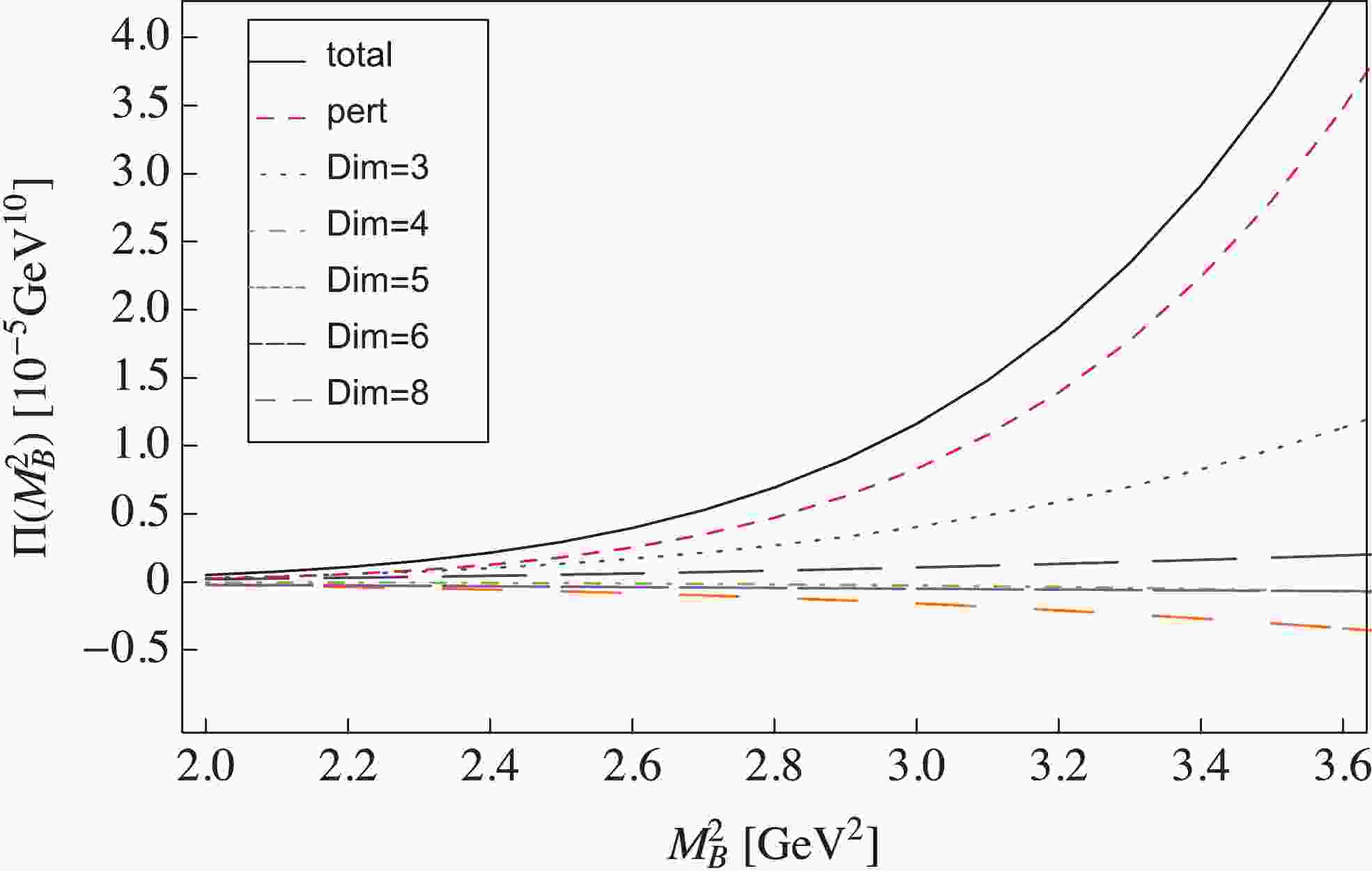
$ \bar{D}_s^\ast D^\ast $ molecular current$ J_{2}(x) $ with$ J^{P} = 0^+ $ as an example to show the details of the numerical analysis. For this current, the dominant non-perturbative contribution to the correlation function comes from the quark condensate$ \langle\bar{q}q\rangle $ and$ \langle\bar{s}s\rangle $ . In Fig. 1, we show the contributions of the perturbative term and various condensate terms to the correlation function. It is clear that the Borel mass$ M_{\rm B}^{2} $ should be large enough to ensure the convergence of the OPE series. Here, we require the highest dimension condensate contribution to be less than 10%,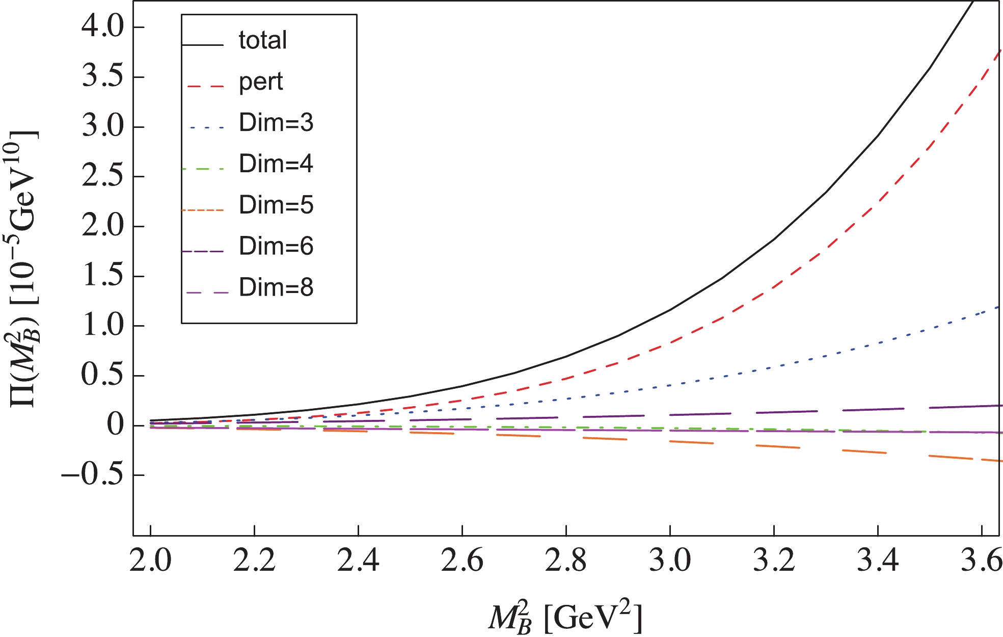
Figure 1. (color online) OPE convergence for the
$ \bar{D}_s^\ast D^\ast $ molecular current$ J_{2}(x) $ with$J^{P} = 0^+ .$ $ {\frac{\Pi^{\langle\bar{q}q\rangle \langle\bar{q}g_{s}\sigma\cdot G q\rangle}(M_{\rm B}^{2},\infty)}{\Pi(M_{\rm B}^{2},\infty)}<10\% } \, , $

(18) which results in
$M_{\rm B}^{2}\geqslant 2.6\;\text{GeV}^{2}$ .As mentioned above, the variation of the output hadron mass
$ m_{H} $ with$ M_{\rm B}^{2} $ should be minimized to obtain the optimized value of the continuum threshold$ s_0 $ . We show the variations of$ m_{H} $ with$ s_{0} $ and$ M_{\rm B}^{2} $ in Fig. 2, from which the dependence of$ m_{H} $ on$ M_{\rm B}^{2} $ can be minimized at$ s_{0}\approx 20.5\;\text{GeV}^{2} $ . Requiring the pole contribution to be larger than 30%, the upper bound on$ M_{\rm B}^{2} $ can then be determined to be$ 3.4\; \text{GeV}^{2} $ . The working region of the Borel parameter for the scalar$ \bar{D}_s^\ast D^\ast $ molecular current$ J_{2}(x) $ is thus$2.6\leqslant M_{\rm B}^{2}\leqslant 3.4\;\text{GeV}^{2}$ . As shown in Fig. 2, the mass sum rules are established to be very stable in these parameter regions, and the hadron mass for the$ \bar{D}_s^\ast D^\ast $ molecule with$ J^{P} = 0^{+} $ can be obtained as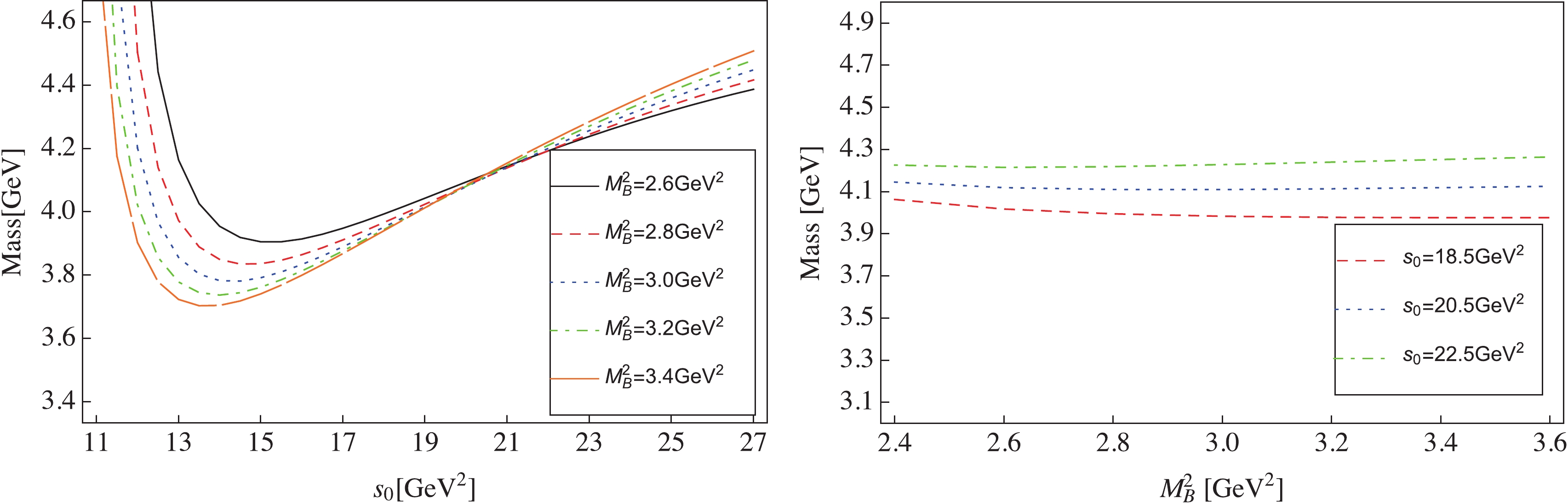
Figure 2. (color online) Variations of
$ m_{H} $ with$ s_{0} $ and$M_{\rm B}^{2}$ corresponding to the current$ J_{2}(x) $ in the$ \bar{D}_s^\ast D^\ast $ system with$J^{P} = 0^{+}.$ $ m_{\bar{D}_s^\ast D^\ast, \, 0^+} = 4.11\pm0.14\; \text{GeV}\, , $

(19) in which the error comes from the uncertainties of the continuum threshold
$ s_{0} $ , Borel mass$ M_{\rm B} $ , the various condensates, and quark masses. After performing similar analyses, we obtain the numerical results for all the other interpolating currents in Eqs. (2) and (3) and present them in Table 1.System Current $ J^{P} $ 

$ s_{0} $ /

$\text{GeV} ^{2} $ 

$ M_{B}^{2} $ /

$ \text{GeV}^{2} $ 

$ m_{H} $ /GeV

PC (%) $ \bar{D}_sD $ 

$ J_{1} $ 

$ 0^{+} $ 

18.0 ± 2.0 1.6 ~ 3.6 3.74 ± 0.13 52.5 $ \bar{D}_s^\ast D^\ast $ 

$ J_{2} $ 

$ 0^{+} $ 

20.5 ± 2.0 2.6 ~ 3.4 4.11 ± 0.14 42.4 $ \bar{D}_s^{*}D $ 

$ J_{1\mu} $ 

$ 1^{+} $ 

20.7 ± 2.0 2.1 ~ 2.5 3.99 ± 0.12 68.2 $ \bar{D}_sD^{*} $ 

$ J_{2\mu} $ 

$ 1^{+} $ 

20.5 ± 2.0 2.1 ~ 2.5 3.97 ± 0.11 67.7 $ \bar{D}_s^\ast D^\ast $ 

$ J_{3\mu} $ 

$ 1^{+} $ 

21.5 ± 2.0 2.8 ~ 3.6 4.22 ± 0.14 40.1 $ \bar{D}_s^\ast D^\ast $ 

$ J_{4\mu} $ 

$ 1^{+} $ 

21.5 ± 2.0 2.8 ~ 3.6 4.22 ± 0.14 40.0 $ \bar{D}_s^\ast D^\ast $ 

$ J_{\mu\nu} $ 

$ 2^{+} $ 

23.0 ± 2.0 2.8 ~ 4.3 4.34 ± 0.13 48.7 $ \mathbf{0}_{[sc]} \oplus \mathbf{0}_{[\bar q \bar{c}]} $ (spin-spin)

$ \eta_{1} $ 

$ 0^{+} $ 

18.0 ± 2.0 2.1 ~ 3.1 3.84 ± 0.15 46.3 $ \mathbf{1}_{[sc]} \oplus \mathbf{1}_{[\bar q \bar{c}]} $ 

$ \eta_{2} $ 

$ 0^{+} $ 

20.0 ± 2.0 2.6 ~ 3.2 4.13 ± 0.17 35.6 $ \mathbf{1}_{[sc]} \oplus \mathbf{0}_{[\bar q \bar{c}]} $ 

$ \eta_{1\mu} $ 

$ 1^{+} $ 

19.0 ± 2.0 2.5 ~ 3.3 3.98 ± 0.16 41.0 $ \mathbf{0}_{[sc]} \oplus \mathbf{1}_{[\bar q \bar{c}]} $ 

$ \eta_{2\mu} $ 

$ 1^{+} $ 

19.0 ± 2.0 2.5 ~ 3.3 3.97 ± 0.15 41.6 $ \mathbf{1}_{[sc]} \oplus \mathbf{1}_{[\bar q \bar{c}]} $ 

$ \eta_{3\mu} $ 

$ 1^{+} $ 

22.0 ± 2.0 2.9 ~ 3.6 4.28 ± 0.14 40.9 $ \mathbf{1}_{[sc]} \oplus \mathbf{1}_{[\bar q \bar{c}]} $ 

$ \eta_{4\mu} $ 

$ 1^{+} $ 

22.0 ± 2.0 2.9 ~ 3.6 4.28 ± 0.14 41.1 $ \mathbf{1}_{[sc]} \oplus \mathbf{1}_{[\bar q \bar{c}]} $ 

$ \eta_{\mu\nu} $ 

$ 2^{+} $ 

23.0 ± 2.0 2.8 ~ 4.3 4.33 ± 0.13 46.4 Table 1. Numerical results for the
$ \bar{D}_s^{(\ast)} D^{(\ast)} $ molecular and diquark-antiquark$ sc\bar q\bar c $ tetraquark systems.In Table 1, the mass of the scalar
$ \bar{D}_sD $ molecular state is predicted to be slightly below the open-charm threshold$ T_{\bar{D}_sD} = 3.84 $ GeV, implying that it can only decay into the hidden-charm channel$ \eta_c K $ . The scalar$ \bar{D}_s^{*} D^{*} $ state is predicted to be very close to$ T_{\bar{D}_s^{*} D^{*}} = 4.12 $ GeV; however, it can decay into$ \bar{D}_sD $ and$ \eta_c K $ final states kinematically in the S-wave. The masses for the$ \bar{D}_{s}^{*} D^{*} $ molecular states with$ J^P = 1^{+}, 2^{+} $ are significantly above the corresponding open-charm thresholds.The masses obtained from the axial-vector molecular currents
$ J_{1\mu} $ and$ J_{2\mu} $ are$ m_{\bar{D}_s^{*}D, \, 1^+} = (3.99 \pm 0.12) $ GeV and$ m_{\bar{D}_{s}D^{*}, \, 1^+} = (3.97 \pm 0.11) $ GeV, which are almost degenerate with each other. One may wonder whether these two currents$ J_{1\mu} $ and$ J_{2\mu} $ could couple to the same physical molecular state or not. In QCD sum rules, this can be specified by studying the following off-diagonal correlation function$ \begin{array}{l} \Pi_{12\mu \nu}^M\left(p^{2}\right) = {\rm i} \int {\rm d}^{4} x {\rm e}^{{\rm i} p \cdot x}\left\langle 0\left|T\left[J_{1\mu}(x) J_{2\nu}^{\dagger}(0)\right]\right| 0\right\rangle\, . \end{array} $

(20) Our calculation shows that this off-diagonal correlation function
$ \Pi_{12\mu \nu}^M\left(p^{2}\right) = 0 $ at the leading order of$ \alpha_s $ for the axial-vector molecular currents$ J_{1\mu} $ and$ J_{2\mu} $ , including the perturbative term and all contributions from various non-perturbative condensates. According to Ref. [43], the NLO perturbative correction is numerically small; thus,$ \Pi_{12\mu \nu}^M\left(p^{2}\right) $ is still negligible compared with the diagonal correlators$ \Pi_{11\mu \nu}^M\left(p^{2}\right) $ and$ \Pi_{22\mu \nu}^M\left(p^{2}\right) $ at the next leading order of$ \alpha_s $ . This result implies that$ J_{1\mu} $ and$ J_{2\mu} $ may couple to different physical states.We also study the
$ sc\bar q\bar c $ tetraquark systems with$ J^P = 0^+, 1^+, 2^+ $ . In Fig. 3, we show the variations of the tetraquark mass with$ s_{0} $ and$ M_{\rm B}^{2} $ for the current$ \eta_{1\mu}(x) $ with$ J^{P} = 1^{+} $ ; the mass sum rules are very stable and reliable in the chosen parameter regions. Regarding the interpolating currents in Eq. (3), we collect the numerical results for these$ sc\bar q\bar c $ tetraquark systems in Table 1. It is shown that the mass spectra for the$ sc\bar q\bar c $ tetraquarks are very similar to the$ \bar{D}_s^{(\ast)} D^{(\ast)} $ molecular states. For the axial-vector$ sc\bar q\bar c $ tetraquark systems, the extracted masses from$ \eta_{1\mu}(x) $ and$ \eta_{2\mu}(x) $ are almost the same as the$ \bar{D}_s^{*}D $ and$ \bar{D}_sD^{*} $ molecular states, which are consistent with the mass of$ Z_{cs}(3985)^- $ from BESIII [1]. It is interesting to examine the off-diagonal correlation function for$ \eta_{1\mu}(x) $ and$ \eta_{2\mu}(x) $ 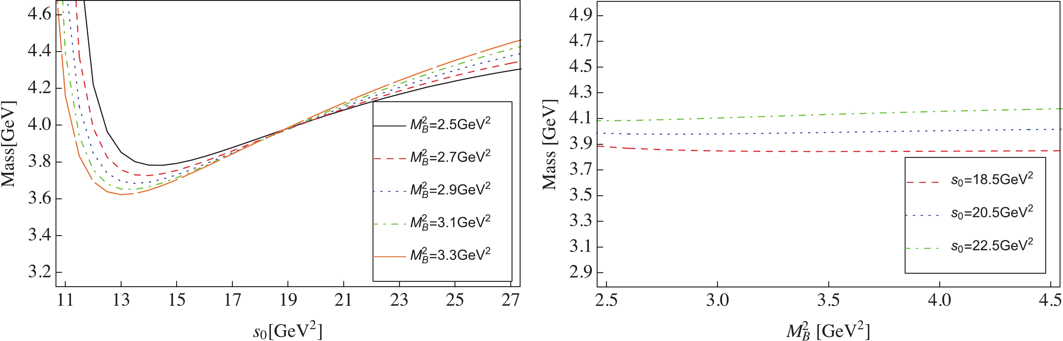
Figure 3. (color online) Variations of
$ m_{H} $ with$ s_{0} $ and$M_{\rm B}^{2}$ for the current$ \eta_{1\mu}(x) $ in the$ sc\bar q\bar c $ tetraquark system with$J^{P} = 1^{+}.$ $ \begin{array}{l} \Pi_{12\mu \nu}^T\left(p^{2}\right) = {\rm i} \int {\rm d}^{4} x {\rm e}^{{\rm i} p \cdot x}\left\langle 0\left|T\left[J_{1\mu}(x) J_{2\nu}^{\dagger}(0)\right]\right| 0\right\rangle\, . \end{array} $

(21) The calculation indicates that the perturbative term and the quark condensate terms in
$ \Pi_{12\mu \nu}^T\left(p^{2}\right) $ are equal to zero, This off-diagonal correlation function$ \Pi_{12\mu \nu}^T\left(p^{2}\right) $ is very small, suggesting that the currents$ \eta_{1\mu}(x) $ and$ \eta_{2\mu}(x) $ cannot strongly couple to the same physical state. -
To study the hidden-charm four-quark systems with strangeness, we have calculated the mass spectra for the
$ \bar{D}_s^{(*)}D^{(*)} $ molecular states and$ sc\bar q\bar c $ tetraquark states with$ J^P = 0^+, 1^+, 2^+ $ in the framework of QCD sum rules. We construct the corresponding molecular and tetraquark interpolating currents and calculate their two-point correlation functions and spectral densities up to dimension eight condensates at the leading order of$ \alpha_s $ . The quark condensates are found to be the most important non-perturbative contribution to the correlation functions for both molecular and tetraquark systems.One may wonder if the two-meson scattering states can contribute to the correlation functions in our calculations. In general, the interpolating currents can couple to all structures with the same quantum numbers, including resonances, two-meson scattering states, and continuum. Thus, these structures will give contributions to the correlation functions. However, it has been demonstrated that the two-meson scattering states cannot saturate the QCD sum rules, while only exotic four-quark states can saturate the QCD sum rules. Moreover, the contributions from the two-meson scattering states to the correlation functions are numerically negligible [43, 55].
Our results show that the masses of the axial-vector
$ \bar{D}_sD^{*} $ ,$ \bar{D}_s^{*}D $ molecular states and the$ sc\bar q\bar c $ tetraquark states from$ \eta_{1\mu} $ ,$ \eta_{2\mu} $ are calculated in good agreement with the mass of$ Z_{cs}(3985)^- $ . In the present calculations, it is difficult to distinguish the nature of$ Z_{cs}(3985)^- $ from the molecular and diquark-antidiquark configurations. In both the molecular and diquark-antidiquark pictures, our results suggest that there may exist two almost degenerate states, as the strange partners of$ X(3872) $ and$ Z_c(3900) $ . We propose to carefully examine$ Z_{cs}(3985) $ in future experiments to verify this. One can search for more hidden-charm four-quark states with strangeness in not only the open-charm$ \bar{D}_s^{(*)}D^{(*)} $ channels but also the hidden-charm channels$ \eta_c K/K^\ast $ ,$ J/\psi K/K^\ast $ .Note added: Since we finished this work, the LHCb Collaboration has reported two new charged resonances,
$ Z_{cs}(4000)^+ $ and$ Z_{cs}(4220)^+ $ , in the$ J/\psi K^+ $ final states [56]. Their masses and decay widths are measured to be$ M_{Z_{cs}(4000)^+} = 4003\pm6^{+4}_{-14} $ MeV and$ \Gamma_{Z_{cs}(4000)^+} = 131\pm15\pm26 $ MeV, and$ M_{Z_{cs}(4220)^+} = 4216\pm24^{+43}_{-30} $ MeV and$ \Gamma_{Z_{cs}(4220)^+} = 233\pm52^{+97}_{-73} $ MeV, respectively, while their spin-parity quantum numbers are identified to prefer$ J^P = 1^+ $ . These masses and spin-parity are consistent with the axial-vector$ \bar{D}_sD^{*} $ ($ \bar{D}_s^{*}D $ ),$ \bar{D}^{*}_sD^{*} $ molecular states and$ \mathbf{1}_{[sc]} \oplus \mathbf{0}_{[\bar q \bar{c}]} $ ($ \mathbf{0}_{[sc]} \oplus \mathbf{1}_{[\bar q \bar{c}]} $ ),$ \mathbf{1}_{[sc]} \oplus \mathbf{1}_{[\bar q \bar{c}]} $ ($ \mathbf{1}_{[sc]} \oplus \mathbf{1}_{[\bar q \bar{c}]} $ ) tetraquark states that we have predicted in Table 1.According to the observation of the LHCb, the decay width of
$ Z_{cs}(4000) $ is much larger than that of$ Z_{cs}(3985) $ observed by BESIII [1]. LHCb found no evidence that$ Z_{cs}(4000) $ and$ Z_{cs}(3985) $ are the same state, although their masses are very close to each other. If this is true, they may be identified as the strange partners of$ X(3872) $ and$ Z_c(3900) $ with$ J^{PC} = 1^{++} $ and$ J^{PC} = 1^{+-} $ , respectively. We propose to carefully examine$ Z_{cs}(4000) $ and$ Z_{cs}(3985) $ in future experiments to verify this. -
In this appendix, we list the spectral densities for the
$ \bar{D}_s^{(*)}D^{(*)} $ and$ sc\bar q\bar c $ systems with$ J^{P} = 0^{+} $ ,$ 1^{+} $ , and$ 2^{+} $ . The spectral density includes the perturbative term, quark condensate, gluon condensate, quark-gluon mixed condensate, four-quark condensate, and dimension eight condensate$ \rho(s) = \rho^{0}(s)+\rho^{3}(s)+\rho^{4}(s)+\rho^{5}(s)+\rho^{6}(s)+\rho^{8}(s)\, , \tag{A1}$

(22) in which the superscripts stand for the dimension of various condensates.
1. Spectral densities for
$ J_{1} $ :$ \rho_{J_{1}}^{0a}(s) = \frac{3} {2048 \pi^{6}}\int_{\alpha_{\rm min}}^{\alpha_{\rm max}} {\rm d} \alpha \int_{\beta_{\rm min}}^{\beta_{\rm max}} {\rm d} \beta \frac{(1-\alpha-\beta)^{2}} { \alpha^{3} \beta^{3}}(m_{c}^{2}(\alpha+\beta)-\alpha \beta s)^{3}(m_{c}^{2}(\alpha+\beta)-3 \alpha \beta s)\, , $ 
$ \rho_{J_{1}}^{0b}(s) = - \frac{3m_{c}} {1024 \pi^{6}}\int_{\alpha_{\rm min}}^{\alpha_{\rm max}} {\rm d} \alpha \int_{\beta_{\rm min}}^{\beta_{\rm max}} {\rm d} \beta (1-\alpha-\beta)^{2}(m_{c}^{2}(\alpha+\beta)-\alpha \beta s)^{2}(2m_{c}^{2}(\alpha+\beta)-5 \alpha \beta s) \left(\frac{m_{s}}{\alpha^{2} \beta^{3}}+\frac{m_{q}}{\alpha^{3} \beta^{2}}\right)\, , $

$ \rho_{J_{1}}^{3a}(s) \!=\! - \frac{3\langle\bar{s}s\rangle}{128\pi^{4} } \!\!\int_{\alpha_{\rm min}}^{\alpha_{\rm max}} {\rm d} \alpha \!\!\int_{\beta_{\rm min}}^{\beta_{\rm max}} {\rm d} \beta (m_{c}^{2}(\alpha+\beta)-\alpha \beta s)\left[\frac{2(1-\alpha-\beta)(m_{c}^{2}(\alpha+\beta)-2\alpha \beta s)m_{c}} { \alpha \beta^{2}} -\frac{2m_{c}^{2}m_{q}+(m_{c}^{2}(\alpha+\beta)-2\alpha \beta s)m_{s}}{\alpha\beta}\right]\, , $

$ \rho_{J_{1}}^{3b}(s) = - \frac{3\langle\bar{q}q\rangle}{128\pi^{4} } \int_{\alpha_{\rm min}}^{\alpha_{\rm max}} {\rm d} \alpha \int_{\beta_{\rm min}}^{\beta_{\rm max}} {\rm d} \beta (m_{c}^{2}(\alpha+\beta)-\alpha \beta s)\left[\frac{2(1-\alpha-\beta)(m_{c}^{2}(\alpha+\beta)-2\alpha \beta s)m_{c}} { \alpha^{2} \beta} -\frac{2m_{c}^{2}m_{s}+(m_{c}^{2}(\alpha+\beta)-2\alpha \beta s)m_{q}}{\alpha\beta}\right]\, ,$

$ \rho_{J_{1}}^{4a}(s) = \frac{\langle g_{s}^{2} G G\rangle m_{c}^{2} }{4096 \pi^{6}}\int_{\alpha_{\rm min}}^{\alpha_{\rm max}} {\rm d} \alpha \int_{\beta_{\rm min}}^{\beta_{\rm max}} {\rm d} \beta (1-\alpha-\beta)^{2} (2m_{c}^{2}(\alpha+ \beta)-3 \alpha \beta s)\left(\frac{1}{\alpha^{3}}+\frac{1}{\beta^{3}}\right)\, , $

$ \rho_{J_{1}}^{4b}(s) = \frac{3\langle g_{s}^{2} G G\rangle m_{c}^{2} }{2048 \pi^{6}}\int_{\alpha_{\rm min}}^{\alpha_{\rm max}} {\rm d} \alpha \int_{\beta_{\rm min}}^{\beta_{\rm max}} {\rm d} \beta (1-\alpha-\beta) (m_{c}^{2}(\alpha+ \beta)-\alpha \beta s)(m_{c}^{2}(\alpha+ \beta)-2\alpha \beta s)\left(\frac{1}{\alpha^{2}\beta}+\frac{1}{\alpha\beta^{2}}\right)\, , $

$ \rho_{J_{1}}^{5a}(s) = \frac{3 \langle\bar{s} g_{s}\sigma\cdot G s\rangle m_{c}}{256 \pi^{4}} \int_{\alpha_{\rm min}}^{\alpha_{\rm max}} {\rm d} \alpha \int_{\beta_{\rm min}}^{\beta_{\rm max}} {\rm d} \beta \left[(2 m_{c}^{2}(\alpha+\beta)-3 s \alpha \beta) \left(\frac{1}{\beta}-\frac{2(1-\alpha-\beta)}{\beta^{2}}\right)+\frac{2m_{c}m_{q}}{\beta}\right]\, , $

$ \rho_{J_{1}}^{5b}(s) = \frac{3 \langle\bar{q} g_{s}\sigma\cdot G q\rangle m_{c}}{256 \pi^{4}} \int_{\alpha_{\rm min}}^{\alpha_{\rm max}} {\rm d} \alpha \int_{\beta_{\rm min}}^{\beta_{\rm max}} {\rm d} \beta \left[(2 m_{c}^{2}(\alpha+\beta)-3 s \alpha \beta) \left(\frac{1}{\alpha}-\frac{2(1-\alpha-\beta)}{\alpha^{2}}\right)+\frac{2m_{c}m_{s}}{\alpha}\right]\, ,$

$ \rho_{J_{1}}^{5c}(s) = \frac{\langle\bar{q} g_{s}\sigma\cdot G q\rangle}{512 \pi^{4}}\left(\left(s-2 m_{c}^{2}\right) m_{q}-6 m_{c}^{2} m_{s}\right) \sqrt{1-\frac{4 m_{c}^{2}}{s}} +\frac{\langle\bar{s} g_{s}\sigma\cdot G s\rangle}{512 \pi^{4}}\left(\left(s-2 m_{c}^{2}\right) m_{s}-6 m_{c}^{2} m_{q}\right) \sqrt{1-\frac{4 m_{c}^{2}}{s}}\, , $

$ \rho_{J_{1}}^{6a}(s) = \frac{\langle\bar{s}s\rangle\langle\bar{q}q\rangle }{32 \pi^{2}}(2m_{c}^{2}+m_{c}m_{q}+m_{c}m_{s}) \sqrt{1-\frac{4 m_{c}^{2}}{s}}\, , $

$ \Pi_{J_{1}}^{6b}\left(M_{\rm B}^{2}\right) = -\frac{\langle\bar{s}s\rangle\langle\bar{q}q\rangle m_{c}^{3}}{32 \pi^{2}} \int_{0}^{1} {\rm d} \alpha\Big(\frac{m_{q}}{1-\alpha}+\frac{m_{s}}{\alpha}\Big) {\rm e}^{\frac{-m_{c}^{2}} { \alpha(1-\alpha) M_{\rm B}^{2}}}\, , $

$ \Pi_{J_{1}}^{8}\left(M_{\rm B}^{2}\right) = \frac{ m_{c}^{4}}{64 \pi^{2}} \int_{0}^{1} {\rm d} \alpha\left(\frac{ \langle\bar{s}s\rangle \langle\bar{q}g_{s}\sigma\cdot Gq\rangle+\langle\bar{q}q\rangle \langle\bar{s}g_{s}\sigma\cdot Gs\rangle}{(1-\alpha)^{2}M_{\rm B}^{2}} -\frac{2 \langle\bar{s}s\rangle \langle\bar{q}g_{s}\sigma\cdot Gq\rangle}{(1-\alpha)m_{c}^{2}}-\frac{ 2\langle\bar{q}q\rangle \langle\bar{s}g_{s}\sigma\cdot Gs\rangle}{\alpha m_{c}^{2}}\right) {\rm e}^{\frac{-m_{c}^{2}} { \alpha(1-\alpha) M_{\rm B}^{2}}}\, , $

where
$ \alpha_{\rm min } = \frac{1}{2}-\frac{1}{2}\sqrt{1-\frac{4 m_{c}^{2}}{s}},\; \; \; \alpha_{\rm max } = \frac{1}{2}+\frac{1}{2}\sqrt{1-\frac{4 m_{c}^{2}}{s}},\; \; \; \beta_{\rm min} = \frac{\alpha m_{c}^{2}}{\alpha s-m_{c}^{2}},\; \; \; \; \beta_{\rm max} = 1-\alpha \, , $

2. Spectral densities for
$ J_{2} $ :$ \rho_{J_{2}}^{0a}(s) = \frac{3} {512 \pi^{6}}\int_{\alpha_{\rm min}}^{\alpha_{\rm max}} {\rm d} \alpha \int_{\beta_{\rm min}}^{\beta_{\rm max}} {\rm d} \beta \frac{(1-\alpha-\beta)^{2}} { \alpha^{3} \beta^{3}}(m_{c}^{2}(\alpha+\beta)-\alpha \beta s)^{3}(m_{c}^{2}(\alpha+\beta)-3 \alpha \beta s)\, , $

$ \rho_{J_{2}}^{0b}(s) = - \frac{3m_{c}} {512 \pi^{6}}\int_{\alpha_{\rm min}}^{\alpha_{\rm max}} {\rm d} \alpha \int_{\beta_{\rm min}}^{\beta_{\rm max}} {\rm d} \beta (1-\alpha-\beta)^{2}(m_{c}^{2}(\alpha+\beta)-\alpha \beta s)^{2}(2m_{c}^{2}(\alpha+\beta)-5 \alpha \beta s) \left(\frac{m_{s}}{\alpha^{2} \beta^{3}}+\frac{m_{q}}{\alpha^{3} \beta^{2}}\right)\, , $

$ \rho_{J_{2}}^{3a}(s) = - \frac{3\langle\bar{s}s\rangle}{64\pi^{4} } \int_{\alpha_{\rm min}}^{\alpha_{\rm max}} {\rm d} \alpha \int_{\beta_{\rm min}}^{\beta_{\rm max}} {\rm d} \beta (m_{c}^{2}(\alpha+\beta)-\alpha \beta s)\left[\frac{2(1-\alpha-\beta)(m_{c}^{2}(\alpha+\beta)-2\alpha \beta s)m_{c}} { \alpha \beta^{2}} -\frac{4m_{c}^{2}m_{q}+(m_{c}^{2}(\alpha+\beta)+2\alpha \beta s)m_{s}}{\alpha\beta}\right]\, , $

$ \rho_{J_{2}}^{3b}(s) = - \frac{3\langle\bar{q}q\rangle}{64\pi^{4} } \int_{\alpha_{\rm min}}^{\alpha_{\rm max}} {\rm d} \alpha \int_{\beta_{\rm min}}^{\beta_{\rm max}} {\rm d} \beta (m_{c}^{2}(\alpha+\beta)-\alpha \beta s)\left[\frac{2(1-\alpha-\beta)(m_{c}^{2}(\alpha+\beta)-2\alpha \beta s)m_{c}} { \alpha^{2} \beta} -\frac{4m_{c}^{2}m_{s}+(m_{c}^{2}(\alpha+\beta)+2\alpha \beta s)m_{q}}{\alpha\beta}\right]\, , $

$ \rho_{J_{2}}^{4}(s) = \frac{\langle g_{s}^{2} G G\rangle m_{c}^{2} }{1024 \pi^{6}}\int_{\alpha_{\rm min}}^{\alpha_{\rm max}} {\rm d} \alpha \int_{\beta_{\rm min}}^{\beta_{\rm max}} {\rm d} \beta (1-\alpha-\beta)^{2} (2m_{c}^{2}(\alpha+ \beta)-3 \alpha \beta s)\left(\frac{1}{\alpha^{3}}+\frac{1}{\beta^{3}}\right)\, , $

$ \rho_{J_{2}}^{5a}(s) = \frac{3 \langle\bar{s} g_{s}\sigma\cdot G s\rangle m_{c}}{128 \pi^{4}} \int_{\alpha_{\rm min}}^{\alpha_{\rm max}} {\rm d} \alpha \int_{\beta_{\rm min}}^{\beta_{\rm max}} {\rm d} \beta \frac{2 m_{c}^{2}(\alpha+\beta)-3 s \alpha \beta}{\beta} +\frac{3 \langle\bar{q} g_{s}\sigma\cdot G q\rangle m_{c}}{128 \pi^{4}} \int_{\alpha_{\rm min}}^{\alpha_{\rm max}} {\rm d} \alpha \int_{\beta_{\rm min}}^{\beta_{\rm max}} {\rm d} \beta \frac{2 m_{c}^{2}(\alpha+\beta)-3 s \alpha \beta }{\alpha}\, , $

$ \rho_{J_{2}}^{5b}(s) = \frac{\langle\bar{q} g_{s}\sigma\cdot G q\rangle}{128 \pi^{4}}\left(\left(s-2 m_{c}^{2}\right) m_{q}-6 m_{c}^{2} m_{s}\right) \sqrt{1-\frac{4 m_{c}^{2}}{s}} +\frac{\langle\bar{s} g_{s}\sigma\cdot G s\rangle}{128 \pi^{4}}\left(\left(s-2 m_{c}^{2}\right) m_{s}-6 m_{c}^{2} m_{q}\right) \sqrt{1-\frac{4 m_{c}^{2}}{s}}\, , $

$ \rho_{J_{2}}^{6a}(s) = \frac{\langle\bar{s}s\rangle\langle\bar{q}q\rangle }{16 \pi^{2}}(4m_{c}^{2}+m_{c}m_{q}+m_{c}m_{s}) \sqrt{1-\frac{4 m_{c}^{2}}{s}}\, , $

$ \Pi_{J_{2}}^{6b}\left(M_{\rm B}^{2}\right) = \frac{\langle\bar{s}s\rangle\langle\bar{q}q\rangle m_{c}^{3}}{16 \pi^{2}} \int_{0}^{1} {\rm d} \alpha\left(\frac{m_{q}}{1-\alpha}+\frac{m_{s}}{\alpha}\right) {\rm e}^{\frac{-m_{c}^{2}} { \alpha(1-\alpha) M_{\rm B}^{2}}}\, , $

$ \Pi_{J_{2}}^{8}\left(M_{\rm B}^{2}\right) = \frac{ m_{c}^{4}}{16 \pi^{2}} \int_{0}^{1} {\rm d} \alpha \frac{ \langle\bar{s}s\rangle \langle\bar{q}g_{s}\sigma\cdot Gq\rangle+\langle\bar{q}q\rangle \langle\bar{s}g_{s}\sigma\cdot Gs\rangle}{(1-\alpha)^{2}M_{\rm B}^{2}} {\rm e}^{\frac{-m_{c}^{2}} { \alpha(1-\alpha) M_{\rm B}^{2}}}\, , $

3. Spectral densities for
$ J_{1\mu} $ :$ \rho_{J_{1\mu}}^{0a}(s) = \frac{3} {4096 \pi^{6}}\int_{\alpha_{\rm min}}^{\alpha_{\rm max}} {\rm d} \alpha \int_{\beta_{\rm min}}^{\beta_{\rm max}} {\rm d} \beta \frac{(1-\alpha-\beta)^{2}} { \alpha^{3} \beta^{3}}(m_{c}^{2}(\alpha+\beta)-\alpha \beta s)^{3}(m_{c}^{2}(\alpha+\beta)-5 \alpha \beta s)\, , $

$ \rho_{J_{1\mu}}^{0b}(s) = - \frac{3m_{c}} {1024 \pi^{6}}\int_{\alpha_{\rm min}}^{\alpha_{\rm max}} {\rm d} \alpha \int_{\beta_{\rm min}}^{\beta_{\rm max}} {\rm d} \beta (1-\alpha-\beta)^{2}(m_{c}^{2}(\alpha+\beta)-\alpha \beta s)^{2} \left(\frac{(2m_{c}^{2}(\alpha+\beta)-5 \alpha \beta s)m_{s}}{\alpha^{3} \beta^{2}}+\frac{(m_{c}^{2}(\alpha+\beta)-4\alpha \beta s)m_{q}}{\alpha^{2} \beta^{3}}\right)\, , $

$ \rho_{J_{1\mu}}^{3a}(s) = - \frac{3\langle\bar{s}s\rangle}{256\pi^{4} } \int_{\alpha_{\rm min}}^{\alpha_{\rm max}} {\rm d} \alpha \int_{\beta_{\rm min}}^{\beta_{\rm max}} {\rm d} \beta (m_{c}^{2}(\alpha+\beta)-\alpha \beta s)\left[\frac{4(1-\alpha-\beta)(m_{c}^{2}(\alpha+\beta)-2\alpha \beta s)m_{c}} { \alpha^{2} \beta} -\frac{4m_{c}^{2}m_{q}+(m_{c}^{2}(\alpha+\beta)-3\alpha \beta s)m_{s}}{\alpha\beta}\right]\, , $

$ \rho_{J_{1\mu}}^{3b}(s) = - \frac{3\langle\bar{q}q\rangle}{256\pi^{4} } \int_{\alpha_{\rm min}}^{\alpha_{\rm max}} {\rm d} \alpha \int_{\beta_{\rm min}}^{\beta_{\rm max}} {\rm d} \beta (m_{c}^{2}(\alpha+\beta)-\alpha \beta s)\left[\frac{2(1-\alpha-\beta)(m_{c}^{2}(\alpha+\beta)-3\alpha \beta s)m_{c}} { \alpha \beta^{2}} -\frac{4m_{c}^{2}m_{s}+(m_{c}^{2}(\alpha+\beta)-3\alpha \beta s)m_{q}}{\alpha\beta}\right]\, , $

$ \rho_{J_{1\mu}}^{4a}(s) = \frac{\langle g_{s}^{2} G G\rangle m_{c}^{2} }{4096 \pi^{6}}\int_{\alpha_{\rm min}}^{\alpha_{\rm max}} {\rm d} \alpha \int_{\beta_{\rm min}}^{\beta_{\rm max}} {\rm d} \beta (1-\alpha-\beta)^{2} (m_{c}^{2}(\alpha+ \beta)-2 \alpha \beta s)\Big(\frac{1}{\alpha^{3}}+\frac{1}{\beta^{3}}\Big)\, , $

$ \rho_{J_{1\mu}}^{4b}(s) = \frac{\langle g_{s}^{2} G G\rangle m_{c}^{2} }{4096 \pi^{6}}\int_{\alpha_{\rm min}}^{\alpha_{\rm max}} {\rm d} \alpha \int_{\beta_{\rm min}}^{\beta_{\rm max}} {\rm d} \beta (1-\alpha-\beta) (m_{c}^{2}(\alpha+ \beta)-\alpha \beta s)\left(\frac{3(m_{c}^{2}(\alpha+ \beta)-3\alpha \beta s)}{\alpha\beta^{2}} -\frac{(3m_{c}^{2}(\alpha+ \beta)-5\alpha \beta s)}{\alpha^{2}\beta}\right)\, , $

$ \rho_{J_{1\mu}}^{5a}(s) = \frac{3 \langle\bar{s} g_{s}\sigma\cdot G s\rangle m_{c}}{256 \pi^{4}} \int_{\alpha_{\rm min}}^{\alpha_{\rm max}} {\rm d} \alpha \int_{\beta_{\rm min}}^{\beta_{\rm max}} {\rm d} \beta \frac{2m_{c}^{2}(\alpha+\beta)-3 \alpha \beta s} {\alpha}\, , $

$ \rho_{J_{1\mu}}^{5b}(s) = \frac{3 \langle\bar{q} g_{s}\sigma\cdot G q\rangle m_{c}}{256 \pi^{4}} \int_{\alpha_{\rm min}}^{\alpha_{\rm max}} {\rm d} \alpha \int_{\beta_{\rm min}}^{\beta_{\rm max}} {\rm d} \beta \left[( m_{c}^{2}(\alpha+\beta)-2 \alpha \beta s ) \left(\frac{1}{\beta}-\frac{2(1-\alpha-\beta)}{\beta^{2}}\right)+\frac{2m_{c}m_{s}}{\beta}\right]\, , $

$ \rho_{J_{1\mu}}^{5c}(s) = \frac{\langle\bar{s} g_{s}\sigma\cdot G s\rangle}{768\pi^{4}}\left(\left(s- m_{c}^{2}\right) m_{s}-9 m_{c}^{2} m_{q}\right) \sqrt{1-\frac{4 m_{c}^{2}}{s}} +\frac{\langle\bar{q} g_{s}\sigma\cdot G q\rangle}{768 \pi^{4}}\left(\left(s- m_{c}^{2}\right) m_{q}-9 m_{c}^{2} m_{s}\right) \sqrt{1-\frac{4 m_{c}^{2}}{s}}\, , $

$ \rho_{J_{1\mu}}^{6a}(s) = \frac{\langle\bar{s}s\rangle\langle\bar{q}q\rangle }{64 \pi^{2}}(4m_{c}^{2}+2m_{c}m_{q}+m_{c}m_{s}) \sqrt{1-\frac{4 m_{c}^{2}}{s}}\, , $

$ \Pi_{J_{1\mu}}^{6b}\left(M_{\rm B}^{2}\right) = -\frac{\langle\bar{s}s\rangle\langle\bar{q}q\rangle m_{c}^{3}}{32 \pi^{2}} \int_{0}^{1} {\rm d} \alpha\left(\frac{m_{s}}{1-\alpha}+\frac{m_{q}}{\alpha}\right) {\rm e}^{\frac{-m_{c}^{2}} { \alpha(1-\alpha) M_{\rm B}^{2}}}\, , $

$ \Pi_{J_{1\mu}}^{8}\left(M_{\rm B}^{2}\right) = \frac{ m_{c}^{4}}{64 \pi^{2}} \int_{0}^{1} {\rm d} \alpha\left(\frac{ \langle\bar{q}q\rangle \langle\bar{s}g_{s}\sigma\cdot Gs\rangle+\langle\bar{s}s\rangle \langle\bar{q}g_{s}\sigma\cdot Gq\rangle}{(1-\alpha)^{2}M_{\rm B}^{2}} -\frac{2 \langle\bar{s}s\rangle \langle\bar{q}g_{s}\sigma\cdot Gq\rangle}{(1-\alpha)m_{c}^{2}}\right) {\rm e}^{\frac{-m_{c}^{2}} { \alpha(1-\alpha) M_{\rm B}^{2}}}\, , $

4. Spectral densities for
$ J_{2\mu} $ :$ \rho_{J_{2\mu}}^{0a}(s) = \frac{3} {4096 \pi^{6}}\int_{\alpha_{\rm min}}^{\alpha_{\rm max}} {\rm d} \alpha \int_{\beta_{\rm min}}^{\beta_{\rm max}} {\rm d} \beta \frac{(1-\alpha-\beta)^{2}} { \alpha^{3} \beta^{3}}(m_{c}^{2}(\alpha+\beta)-\alpha \beta s)^{3}(m_{c}^{2}(\alpha+\beta)-5 \alpha \beta s)\, , $

$ \rho_{J_{2\mu}}^{0b}(s) = - \frac{3m_{c}} {1024 \pi^{6}}\int_{\alpha_{\rm min}}^{\alpha_{\rm max}} {\rm d} \alpha \int_{\beta_{\rm min}}^{\beta_{\rm max}} {\rm d} \beta (1-\alpha-\beta)^{2}(m_{c}^{2}(\alpha+\beta)-\alpha \beta s)^{2} \Big(\frac{(2m_{c}^{2}(\alpha+\beta)-5 \alpha \beta s)m_{q}}{\alpha^{2} \beta^{3}} +\frac{(m_{c}^{2}(\alpha+\beta)-4\alpha \beta s)m_{s}}{\alpha^{3} \beta^{2}}\Big)\, , $

$ \rho_{J_{2\mu}}^{3a}(s) = - \frac{3\langle\bar{q}q\rangle}{256\pi^{4} } \int_{\alpha_{\rm min}}^{\alpha_{\rm max}} {\rm d} \alpha \int_{\beta_{\rm min}}^{\beta_{\rm max}} {\rm d} \beta (m_{c}^{2}(\alpha+\beta)-\alpha \beta s)\left[\frac{4(1-\alpha-\beta)(m_{c}^{2}(\alpha+\beta)-2\alpha \beta s)m_{c}} { \alpha\beta^{2} } -\frac{4m_{c}^{2}m_{s}+(m_{c}^{2}(\alpha+\beta)-3\alpha \beta s)m_{q}}{\alpha\beta}\right]\, , $

$ \rho_{J_{2\mu}}^{3b}(s) = - \frac{3\langle\bar{s}s\rangle}{256\pi^{4} } \int_{\alpha_{\rm min}}^{\alpha_{\rm max}} {\rm d} \alpha \int_{\beta_{\rm min}}^{\beta_{\rm max}} {\rm d} \beta (m_{c}^{2}(\alpha+\beta)-\alpha \beta s)\left[\frac{2(1-\alpha-\beta)(m_{c}^{2}(\alpha+\beta)-3\alpha \beta s)m_{c}} { \alpha ^{2} \beta} -\frac{4m_{c}^{2}m_{q}+(m_{c}^{2}(\alpha+\beta)-3\alpha \beta s)m_{s}}{\alpha\beta}\right]\, , $

$ \rho_{J_{2\mu}}^{4a}(s) = \frac{\langle g_{s}^{2} G G\rangle m_{c}^{2} }{4096 \pi^{6}}\int_{\alpha_{\rm min}}^{\alpha_{\rm max}} {\rm d} \alpha \int_{\beta_{\rm min}}^{\beta_{\rm max}} {\rm d} \beta (1-\alpha-\beta)^{2} (m_{c}^{2}(\alpha+ \beta)-2 \alpha \beta s)\left(\frac{1}{\alpha^{3}}+\frac{1}{\beta^{3}}\right)\, , $

$ \rho_{J_{2\mu}}^{4b}(s) = \frac{\langle g_{s}^{2} G G\rangle m_{c}^{2} }{4096 \pi^{6}}\int_{\alpha_{\rm min}}^{\alpha_{\rm max}} {\rm d} \alpha \int_{\beta_{\rm min}}^{\beta_{\rm max}} {\rm d} \beta (1-\alpha-\beta) (m_{c}^{2}(\alpha+ \beta)-\alpha \beta s)\left(\frac{3(m_{c}^{2}(\alpha+ \beta)-3\alpha \beta s)}{\alpha^{2} \beta} -\frac{(3m_{c}^{2}(\alpha+ \beta)-5\alpha \beta s)}{\alpha\beta^{2} }\right)\, , $

$ \rho_{J_{2\mu}}^{5a}(s) = \frac{3 \langle\bar{q} g_{s}\sigma\cdot G q\rangle m_{c}}{256 \pi^{4}} \int_{\alpha_{\rm min}}^{\alpha_{\rm max}} {\rm d} \alpha \int_{\beta_{\rm min}}^{\beta_{\rm max}} {\rm d} \beta \frac{2m_{c}^{2}(\alpha+\beta)-3 \alpha \beta s} {\beta}\, , $

$ \rho_{J_{2\mu}}^{5b}(s) = \frac{3 \langle\bar{s} g_{s}\sigma\cdot G s\rangle m_{c}}{256 \pi^{4}} \int_{\alpha_{\rm min}}^{\alpha_{\rm max}} {\rm d} \alpha \int_{\beta_{\rm min}}^{\beta_{\rm max}} {\rm d} \beta \left[( m_{c}^{2}(\alpha+\beta)-2 \alpha \beta s ) \left(\frac{1}{\alpha}-\frac{2(1-\alpha-\beta)}{\alpha^{2}}\right)+\frac{2m_{c}m_{q}}{\alpha}\right]\, , $

$ \rho_{J_{2\mu}}^{5c}(s) = \frac{\langle\bar{s} g_{s}\sigma\cdot G s\rangle}{768\pi^{4}}\left(\left(s- m_{c}^{2}\right) m_{s}-9 m_{c}^{2} m_{q}\right) \sqrt{1-\frac{4 m_{c}^{2}}{s}} +\frac{\langle\bar{q} g_{s}\sigma\cdot G q\rangle}{768 \pi^{4}}\left(\left(s- m_{c}^{2}\right) m_{q}-9 m_{c}^{2} m_{s}\right) \sqrt{1-\frac{4 m_{c}^{2}}{s}}\, , $

$ \rho_{J_{2\mu}}^{6a}(s) = \frac{\langle\bar{s}s\rangle\langle\bar{q}q\rangle }{64 \pi^{2}}(4m_{c}^{2}+2m_{c}m_{s}+m_{c}m_{q}) \sqrt{1-\frac{4 m_{c}^{2}}{s}}\, , $

$ \Pi_{J_{2\mu}}^{6b}\left(M_{\rm B}^{2}\right) = -\frac{\langle\bar{s}s\rangle\langle\bar{q}q\rangle m_{c}^{3}}{32 \pi^{2}} \int_{0}^{1} {\rm d} \alpha\left(\frac{m_{s}}{1-\alpha}+\frac{m_{q}}{\alpha}\right) {\rm e}^{\frac{-m_{c}^{2}} { \alpha(1-\alpha) M_{\rm B}^{2}}}\, , $

$ \Pi_{J_{2\mu}}^{8}\left(M_{\rm B}^{2}\right) = \frac{ m_{c}^{4}}{64 \pi^{2}} \int_{0}^{1} {\rm d} \alpha\left(\frac{ \langle\bar{q}q\rangle \langle\bar{s}g_{s}\sigma\cdot Gs\rangle+\langle\bar{s}s\rangle \langle\bar{q}g_{s}\sigma\cdot Gq\rangle}{(1-\alpha)^{2}M_{\rm B}^{2}} -\frac{2 \langle\bar{q}q\rangle \langle\bar{s}g_{s}\sigma\cdot Gs\rangle}{(1-\alpha)m_{c}^{2}}\right) {\rm e}^{\frac{-m_{c}^{2}} { \alpha(1-\alpha) M_{\rm B}^{2}}}\, , $

5. Spectral densities for
$ J_{3\mu} $ :$ \rho_{J_{3\mu}}^{0a}(s) = \frac{9} {4096 \pi^{6}}\int_{\alpha_{\rm min}}^{\alpha_{\rm max}} {\rm d} \alpha \int_{\beta_{\rm min}}^{\beta_{\rm max}} {\rm d} \beta \frac{(1-\alpha-\beta)^{2}} { \alpha^{3} \beta^{3}}(m_{c}^{2}(\alpha+\beta)-\alpha \beta s)^{3}(m_{c}^{2}(\alpha+\beta)-5 \alpha \beta s)\, , $

$\rho_{J_{3\mu}}^{0b}(s) = - \frac{9m_{c}} {1024 \pi^{6}}\int_{\alpha_{\rm min}}^{\alpha_{\rm max}} {\rm d} \alpha \int_{\beta_{\rm min}}^{\beta_{\rm max}} {\rm d} \beta (1-\alpha-\beta)^{2}(m_{c}^{2}(\alpha+\beta)-\alpha \beta s)^{2} \left(\frac{(m_{c}^{2}(\alpha+\beta)-2\alpha \beta s)m_{q}}{\alpha^{3} \beta^{2}}-\frac{ \alpha \beta sm_{s}}{\alpha^{2} \beta^{3}}\right)\, , $

$ \rho_{J_{3\mu}}^{3a}(s) = \frac{3\langle\bar{s}s\rangle}{256\pi^{4} } \int_{\alpha_{\rm min}}^{\alpha_{\rm max}} {\rm d} \alpha \int_{\beta_{\rm min}}^{\beta_{\rm max}} {\rm d} \beta (m_{c}^{2}(\alpha+\beta)-\alpha \beta s)\left[\frac{4(1-\alpha-\beta) s m_{c}} { \beta}+\frac{12m_{c}^{2}m_{q}+3(m_{c}^{2}(\alpha+\beta)-3\alpha \beta s)m_{s}}{\alpha\beta}\right]\, , $

$ \rho_{J_{3\mu}}^{3b}(s) \!=\! - \frac{3\langle\bar{q}q\rangle}{256\pi^{4} } \!\!\int_{\alpha_{\rm min}}^{\alpha_{\rm max}}\! {\rm d} \alpha \!\!\int_{\beta_{\rm min}}^{\beta_{\rm max}} \!{\rm d} \beta (m_{c}^{2}(\alpha\!+\!\beta)\!-\!\alpha \beta s)\left[\frac{2(1\!-\!\alpha-\beta)(3m_{c}^{2}(\alpha\!+\!\beta)\!-\!5\alpha \beta s)m_{c}} { \alpha^{2} \beta}\!-\!\frac{12m_{c}^{2}m_{s}\! +\! 3(m_{c}^{2}(\alpha\!+\!\beta)\!-\!3\alpha \beta s)m_{q}}{\alpha\beta}\right]\, , $

$ \rho_{J_{3\mu}}^{4a}(s) = \frac{3\langle g_{s}^{2} G G\rangle m_{c}^{2} }{4096 \pi^{6}}\int_{\alpha_{\rm min}}^{\alpha_{\rm max}} {\rm d} \alpha \int_{\beta_{\rm min}}^{\beta_{\rm max}} {\rm d} \beta (1-\alpha-\beta)^{2} (m_{c}^{2}(\alpha+ \beta)-2 \alpha \beta s)\left(\frac{1}{\alpha^{3}}+\frac{1}{\beta^{3}}\right)\, , $

$\rho_{J_{3\mu}}^{4b}(s) = \frac{\langle g_{s}^{2} G G\rangle }{4096 \pi^{6}}\int_{\alpha_{\rm min}}^{\alpha_{\rm max}} {\rm d} \alpha \int_{\beta_{\rm min}}^{\beta_{\rm max}} {\rm d} \beta (1-\alpha-\beta) (m_{c}^{2}(\alpha+ \beta)-\alpha \beta s)\left(\frac{3m_{c}^{2}(\alpha+ \beta)-5\alpha \beta s}{\alpha\beta^{2}} -\frac{3(m_{c}^{2}(\alpha+ \beta)-3\alpha \beta s)}{\alpha^{2}\beta}\right)\, , $

$ \rho_{J_{3\mu}}^{5a}(s) = -\frac{3 \langle\bar{s} g_{s}\sigma\cdot G s\rangle m_{c}}{256 \pi^{4}} \int_{\alpha_{\rm min}}^{\alpha_{\rm max}} {\rm d} \alpha \int_{\beta_{\rm min}}^{\beta_{\rm max}} {\rm d} \beta s \alpha \, , $

$ \rho_{J_{3\mu}}^{5b}(s) = \frac{ \langle\bar{q} g_{s}\sigma\cdot G q\rangle m_{c}}{256 \pi^{4}} \int_{\alpha_{\rm min}}^{\alpha_{\rm max}} {\rm d} \alpha \int_{\beta_{\rm min}}^{\beta_{\rm max}} {\rm d} \beta \left[(3 m_{c}^{2}(\alpha+\beta)-4 s \alpha \beta) \left(\frac{3}{\alpha}+\frac{2(1-\alpha-\beta)}{\alpha^{2}}\right)-\frac{6m_{c}m_{s}}{\alpha}\right]\, , $

$ \rho_{J_{3\mu}}^{5c}(s) = \frac{\langle\bar{q} g_{s}\sigma\cdot G q\rangle}{256\pi^{4}}\left(\left(s- m_{c}^{2}\right) m_{q}-9 m_{c}^{2} m_{s}\right) \sqrt{1-\frac{4 m_{c}^{2}}{s}} +\frac{\langle\bar{s} g_{s}\sigma\cdot G s\rangle}{256 \pi^{4}}\left(\left(s- m_{c}^{2}\right) m_{s}-9 m_{c}^{2} m_{q}\right) \sqrt{1-\frac{4 m_{c}^{2}}{s}}\, , $

$ \rho_{J_{3\mu}}^{6a}(s) = \frac{3\langle\bar{s}s\rangle\langle\bar{q}q\rangle }{64 \pi^{2}}(4m_{c}^{2}+m_{c}m_{s}) \sqrt{1-\frac{4 m_{c}^{2}}{s}}\, , $

$ \Pi_{J_{3\mu}}^{6b}\left(M_{\rm B}^{2}\right) = \frac{\langle\bar{s}s\rangle\langle\bar{q}q\rangle m_{c}^{3}}{32 \pi^{2}} \int_{0}^{1} {\rm d} \alpha\Big(\frac{m_{q}}{1-\alpha}+\frac{m_{s}}{\alpha}\Big) {\rm e}^{\frac{-m_{c}^{2}} { \alpha(1-\alpha) M_{\rm B}^{2}}}\, , $

$ \Pi_{J_{3\mu}}^{8}\left(M_{\rm B}^{2}\right) = \frac{ m_{c}^{4}}{64 \pi^{2}} \int_{0}^{1} {\rm d} \alpha\left(\frac{ 3(\langle\bar{s}s\rangle \langle\bar{q}g_{s}\sigma\cdot Gq\rangle+\langle\bar{q}q\rangle \langle\bar{s}g_{s}\sigma\cdot Gs\rangle)}{(1-\alpha)^{2}M_{\rm B}^{2}} +\frac{2 \langle\bar{s}s\rangle \langle\bar{q}g_{s}\sigma\cdot Gq\rangle}{(1-\alpha)m_{c}^{2}}\right) {\rm e}^{\frac{-m_{c}^{2}} { \alpha(1-\alpha) M_{\rm B}^{2}}}\, , $

6. Spectral densities for
$ J_{4\mu} $ :$ \rho_{J_{4\mu}}^{0a}(s) = \frac{9} {4096 \pi^{6}}\int_{\alpha_{\rm min}}^{\alpha_{\rm max}} {\rm d} \alpha \int_{\beta_{\rm min}}^{\beta_{\rm max}} {\rm d} \beta \frac{(1-\alpha-\beta)^{2}} { \alpha^{3} \beta^{3}}(m_{c}^{2}(\alpha+\beta)-\alpha \beta s)^{3}(m_{c}^{2}(\alpha+\beta)-5 \alpha \beta s)\, , $

$ \rho_{J_{4\mu}}^{0b}(s) = - \frac{9m_{c}} {1024 \pi^{6}}\int_{\alpha_{\rm min}}^{\alpha_{\rm max}} {\rm d} \alpha \int_{\beta_{\rm min}}^{\beta_{\rm max}} {\rm d} \beta (1-\alpha-\beta)^{2}(m_{c}^{2}(\alpha+\beta)-\alpha \beta s)^{2} \left(\frac{(m_{c}^{2}(\alpha+\beta)-2\alpha \beta s)m_{s}}{\alpha^{2} \beta^{3}}-\frac{ \alpha \beta sm_{q}}{\alpha^{3} \beta^{2}}\right)\, , $

$ \rho_{J_{4\mu}}^{3a}(s) = \frac{3\langle\bar{q}q\rangle}{256\pi^{4} } \int_{\alpha_{\rm min}}^{\alpha_{\rm max}} {\rm d} \alpha \int_{\beta_{\rm min}}^{\beta_{\rm max}} {\rm d} \beta (m_{c}^{2}(\alpha+\beta)-\alpha \beta s)\left[\frac{4(1-\alpha-\beta) s m_{c}} { \alpha}+\frac{12m_{c}^{2}m_{s}+3(m_{c}^{2}(\alpha+\beta)-3\alpha \beta s)m_{q}}{\alpha\beta}\right]\, , $

$ \rho_{J_{4\mu}}^{3b}(s) \!=\! - \frac{3\langle\bar{s}s\rangle}{256\pi^{4} } \!\int_{\alpha_{\rm min}}^{\alpha_{\rm max}} \!{\rm d} \alpha \!\int_{\beta_{\rm min}}^{\beta_{\rm max}} \!{\rm d} \beta (m_{c}^{2}(\alpha\!+\! \beta)\! -\! \alpha \beta s)\left[\frac{2(1\! -\! \alpha\! -\! \beta)(3m_{c}^{2}(\alpha\! +\! \beta)\! -\! 5\alpha \beta s)m_{c}} { \alpha \beta^{2}} \! -\! \frac{12m_{c}^{2}m_{q}\! +\! 3(m_{c}^{2}(\alpha\! +\! \beta)\! -\! 3\alpha \beta s)m_{s}}{\alpha\beta}\right]\, , $

$ \rho_{J_{4\mu}}^{4a}(s) = \frac{3\langle g_{s}^{2} G G\rangle m_{c}^{2} }{4096 \pi^{6}}\int_{\alpha_{\rm min}}^{\alpha_{\rm max}} {\rm d} \alpha \int_{\beta_{\rm min}}^{\beta_{\rm max}} {\rm d} \beta (1-\alpha-\beta)^{2} (m_{c}^{2}(\alpha+ \beta)-2 \alpha \beta s)\left(\frac{1}{\alpha^{3}}+\frac{1}{\beta^{3}}\right)\, , $

$\rho_{J_{4\mu}}^{4b}(s) = \frac{\langle g_{s}^{2} G G\rangle }{4096 \pi^{6}}\int_{\alpha_{\rm min}}^{\alpha_{\rm max}} {\rm d} \alpha \int_{\beta_{\rm min}}^{\beta_{\rm max}} {\rm d} \beta (1-\alpha-\beta) (m_{c}^{2}(\alpha+ \beta)-\alpha \beta s)\left(\frac{3m_{c}^{2}(\alpha+ \beta)-5\alpha \beta s}{\alpha^{2}\beta} -\frac{3(m_{c}^{2}(\alpha+ \beta)-3\alpha \beta s)}{\alpha\beta^{2}}\right)\, , $

$ \rho_{J_{4\mu}}^{5a}(s) = -\frac{3 \langle\bar{q} g_{s}\sigma\cdot G q\rangle m_{c}}{256 \pi^{4}} \int_{\alpha_{\rm min}}^{\alpha_{\rm max}} {\rm d} \alpha \int_{\beta_{\rm min}}^{\beta_{\rm max}} {\rm d} \beta s \beta \, , $

$ \rho_{J_{4\mu}}^{5b}(s) = \frac{ \langle\bar{s} g_{s}\sigma\cdot G s\rangle m_{c}}{256 \pi^{4}} \int_{\alpha_{\rm min}}^{\alpha_{\rm max}} {\rm d} \alpha \int_{\beta_{\rm min}}^{\beta_{\rm max}} {\rm d} \beta \left[(3 m_{c}^{2}(\alpha+\beta)-4 s \alpha \beta) \left(\frac{3}{\beta}+\frac{2(1-\alpha-\beta)}{\beta^{2}}\right)-\frac{6m_{c}m_{q}}{\beta}\right]\, , $

$ \rho_{J_{4\mu}}^{5c}(s) = \frac{\langle\bar{s} g_{s}\sigma\cdot G s\rangle}{256\pi^{4}}\left(\left(s- m_{c}^{2}\right) m_{s}-9 m_{c}^{2} m_{q}\right) \sqrt{1-\frac{4 m_{c}^{2}}{s}}+\frac{\langle\bar{q} g_{s}\sigma\cdot G q\rangle}{256 \pi^{4}}\left(\left(s- m_{c}^{2}\right) m_{q}-9 m_{c}^{2} m_{s}\right) \sqrt{1-\frac{4 m_{c}^{2}}{s}}\, , $

$ \rho_{J_{4\mu}}^{6a}(s) = \frac{3\langle\bar{s}s\rangle\langle\bar{q}q\rangle }{64 \pi^{2}}(4m_{c}^{2}+m_{c}m_{q}) \sqrt{1-\frac{4 m_{c}^{2}}{s}}\, , $

$ \Pi_{J_{4\mu}}^{6b}\left(M_{\rm B}^{2}\right) = \frac{\langle\bar{s}s\rangle\langle\bar{q}q\rangle m_{c}^{3}}{32 \pi^{2}} \int_{0}^{1} {\rm d} \alpha\Big(\frac{m_{s}}{1-\alpha}+\frac{m_{q}}{\alpha}\Big) {\rm e}^{\frac{-m_{c}^{2}} { \alpha(1-\alpha) M_{\rm B}^{2}}}\, , $

$ \Pi_{J_{4\mu}}^{8}\left(M_{\rm B}^{2}\right) = \frac{ m_{c}^{4}}{64 \pi^{2}} \int_{0}^{1} {\rm d} \alpha\Big(\frac{ 3(\langle\bar{s}s\rangle \langle\bar{q}g_{s}\sigma\cdot Gq\rangle+\langle\bar{q}q\rangle \langle\bar{s}g_{s}\sigma\cdot Gs\rangle)}{(1-\alpha)^{2}M_{\rm B}^{2}} +\frac{2 \langle\bar{q}q\rangle \langle\bar{s}g_{s}\sigma\cdot Gs\rangle}{(1-\alpha)m_{c}^{2}}\Big) {\rm e}^{\frac{-m_{c}^{2}} { \alpha(1-\alpha) M_{\rm B}^{2}}}\, , $

7. Spectral densities for
$ J_{\mu\nu} $ :$ \rho_{J_{\mu\nu}}^{0a}(s) = -\frac{5} {1024 \pi^{6}}\int_{\alpha_{\rm min}}^{\alpha_{\rm max}} {\rm d} \alpha \int_{\beta_{\rm min}}^{\beta_{\rm max}} {\rm d} \beta \frac{(1-\alpha-\beta)^{2}} { \alpha^{3} \beta^{3}}(m_{c}^{2}(\alpha+\beta)-\alpha \beta s)^{3}\left((\alpha+\beta+2)(m_{c}^{2}(\alpha+\beta)-\alpha \beta s) -3(m_{c}^{2}(\alpha+\beta)-3 \alpha \beta s)\right)\, $

$ \rho_{J_{\mu\nu}}^{0b}(s) = - \frac{15m_{c}} {512 \pi^{6}}\int_{\alpha_{\rm min}}^{\alpha_{\rm max}} {\rm d} \alpha \int_{\beta_{\rm min}}^{\beta_{\rm max}} {\rm d} \beta (1-\alpha-\beta)^{2}(m_{c}^{2}(\alpha+\beta)-\alpha \beta s)^{2}(m_{c}^{2}(\alpha+\beta)-4 \alpha \beta s) \left(\frac{m_{s}}{\alpha^{2} \beta^{3}}+\frac{m_{q}}{\alpha^{3} \beta^{2}}\right)\, , $

$ \begin{aligned}[b] \rho_{J_{\mu\nu}}^{3a}(s) = &- \frac{15\langle\bar{s}s\rangle}{64\pi^{4} } \int_{\alpha_{\rm min}}^{\alpha_{\rm max}} {\rm d} \alpha \int_{\beta_{\rm min}}^{\beta_{\rm max}} {\rm d} \beta (m_{c}^{2}(\alpha+\beta)-\alpha \beta s)\left[\frac{(1-\alpha-\beta)(m_{c}^{2}(\alpha+\beta)-3\alpha \beta s)m_{c}} { \alpha \beta^{2}} \right. \\ &\left.-\frac{2m_{c}^{2}m_{q}-\alpha \beta s m_{s}+(1-\alpha-\beta)(m_{c}^{2}(\alpha+\beta)-s\alpha\beta)m_{s}}{\alpha\beta}\right]\, ,\end{aligned} $

$ \begin{aligned}[b] \rho_{J_{\mu\nu}}^{3b}(s) = & - \frac{15\langle\bar{q}q\rangle}{64\pi^{4} } \int_{\alpha_{\rm min}}^{\alpha_{\rm max}} {\rm d} \alpha \int_{\beta_{\rm min}}^{\beta_{\rm max}} {\rm d} \beta (m_{c}^{2}(\alpha+\beta)-\alpha \beta s)\left[\frac{(1-\alpha-\beta)(m_{c}^{2}(\alpha+\beta)-3\alpha \beta s)m_{c}} { \alpha \beta^{2}}\right.\\ &\left. -\frac{2m_{c}^{2}m_{s}-\alpha \beta s m_{q}+(1-\alpha-\beta)(m_{c}^{2}(\alpha+\beta)-s\alpha\beta)m_{q}}{\alpha\beta}\right]\, , \end{aligned} $

$ \rho_{J_{\mu\nu}}^{4a}(s) = \frac{5 \langle g_{s}^{2} G G\rangle m_{c}^{2} }{1024 \pi^{6}}\int_{\alpha_{\rm min}}^{\alpha_{\rm max}} {\rm d} \alpha \int_{\beta_{\rm min}}^{\beta_{\rm max}} {\rm d} \beta (1-\alpha-\beta)^{2}\left[ (1-\alpha-\beta)(m_{c}^{2}(\alpha+ \beta)- \alpha \beta s)\left(\frac{1}{3\alpha^{3}}+\frac{1}{3\beta^{3}}\right) -\left(\frac{\beta s}{2\alpha^{2}}+\frac{\alpha s}{2\beta^{2}}\right)\right]\, , $

$ \begin{aligned}[b] \rho_{J_{\mu\nu}}^{4b}(s) =& \frac{5\langle g_{s}^{2} G G\rangle m_{c}^{2} }{2048 \pi^{6}}\int_{\alpha_{\rm min}}^{\alpha_{\rm max}} {\rm d} \alpha \int_{\beta_{\rm min}}^{\beta_{\rm max}} {\rm d} \beta (1-\alpha-\beta)(m_{c}^{2}(\alpha+ \beta)-\alpha \beta s)\left(\frac{1}{\alpha^{2}\beta}+\frac{1}{\alpha\beta^{2}}\right)\\ &\times\left((1-\alpha-\beta)(m_{c}^{2}(\alpha+ \beta)- \alpha \beta s)-4(m_{c}^{2}(\alpha+ \beta)-2 \alpha \beta s)\right)\, , \end{aligned} $

$ \begin{aligned}[b] \rho_{J_{\mu\nu}}^{5a}(s) = &\frac{5 \langle\bar{s} g_{s}\sigma\cdot G s\rangle m_{c}}{128 \pi^{4}} \int_{\alpha_{\rm min}}^{\alpha_{\rm max}} {\rm d} \alpha \int_{\beta_{\rm min}}^{\beta_{\rm max}} {\rm d} \beta \frac{3( m_{c}^{2}(\alpha+\beta)-2 \alpha \beta s)m_{c}+2( 2m_{c}^{2}(\alpha+\beta)-3 \alpha \beta s)m_{s}}{\beta}\, ,\\ &+\frac{5 \langle\bar{q} g_{s}\sigma\cdot G q\rangle m_{c}}{128 \pi^{4}} \int_{\alpha_{\rm min}}^{\alpha_{\rm max}} {\rm d} \alpha \int_{\beta_{\rm min}}^{\beta_{\rm max}} {\rm d} \beta \frac{3( m_{c}^{2}(\alpha+\beta)-2 \alpha \beta s)m_{c}+2( 2m_{c}^{2}(\alpha+\beta)-3 \alpha \beta s)m_{q}}{\alpha}\, , \end{aligned} $

$ \rho_{J_{\mu\nu}}^{5b}(s) = \frac{5\langle\bar{q} g_{s}\sigma\cdot G q\rangle}{256 \pi^{4}}\left(\left(s-2 m_{c}^{2}\right) m_{q}-30 m_{c}^{2} m_{s}\right) \sqrt{1-\frac{4 m_{c}^{2}}{s}} +\frac{5\langle\bar{s} g_{s}\sigma\cdot G s\rangle}{256 \pi^{4}}\left(\left(s-2 m_{c}^{2}\right) m_{s}-30 m_{c}^{2} m_{q}\right) \sqrt{1-\frac{4 m_{c}^{2}}{s}}\, , $

$ \rho_{J_{\mu\nu}}^{6a}(s) = \frac{5\langle\bar{s}s\rangle\langle\bar{q}q\rangle }{32 \pi^{2}}(4m_{c}^{2}+m_{c}m_{q}+m_{c}m_{s}) \sqrt{1-\frac{4 m_{c}^{2}}{s}}\, , $

$ \Pi_{J_{\mu\nu}}^{6b}\left(M_{\rm B}^{2}\right) = \frac{5\langle\bar{s}s\rangle\langle\bar{q}q\rangle m_{c}^{3}}{16 \pi^{2}} \int_{0}^{1} {\rm{d}} \alpha\Big(\frac{m_{q}}{1-\alpha}+\frac{m_{s}}{\alpha}\Big) {\rm e}^{\frac{-m_{c}^{2}} { \alpha(1-\alpha) M_{\rm B}^{2}}}\, , $

$ \Pi_{J_{\mu\nu}}^{8}\left(M_{\rm B}^{2}\right) = \frac{ 5m_{c}^{4}}{32 \pi^{2}} \int_{0}^{1} {\rm d} \alpha \frac{ \langle\bar{s}s\rangle \langle\bar{q}g_{s}\sigma\cdot Gq\rangle+\langle\bar{q}q\rangle \langle\bar{s}g_{s}\sigma\cdot Gs\rangle}{(1-\alpha)^{2}M_{\rm B}^{2}} {\rm e}^{\frac{-m_{c}^{2}} { \alpha(1-\alpha) M_{\rm B}^{2}}}\, , $

8. Spectral densities for
$ \eta_{3\mu} $ :$ \rho_{\eta_{3\mu}}^{0a}(s) = \frac{3} {1024 \pi^{6}}\int_{\alpha_{\rm min}}^{\alpha_{\rm max}} {\rm d} \alpha \int_{\beta_{\rm min}}^{\beta_{\rm max}} {\rm d} \beta \frac{(1-\alpha-\beta)^{2}} { \alpha^{3} \beta^{3}}(m_{c}^{2}(\alpha+\beta)-\alpha \beta s)^{3}(m_{c}^{2}(\alpha+\beta)-5 \alpha \beta s)\, , $

$ \rho_{\eta_{3\mu}}^{0b}(s) = - \frac{3m_{c}} {256 \pi^{6}}\int_{\alpha_{\rm min}}^{\alpha_{\rm max}} {\rm d} \alpha \int_{\beta_{\rm min}}^{\beta_{\rm max}} {\rm d} \beta (1-\alpha-\beta)^{2}(m_{c}^{2}(\alpha+\beta)-\alpha \beta s)^{2} \left(\frac{(m_{c}^{2}(\alpha+\beta)-2\alpha \beta s)m_{s}}{\alpha^{3} \beta^{2}}-\frac{ \alpha \beta sm_{q}}{\alpha^{2} \beta^{3}}\right)\, , $

$ \rho_{\eta_{3\mu}}^{3a}(s) = \frac{\langle\bar{q}q\rangle}{64\pi^{4} } \int_{\alpha_{\rm min}}^{\alpha_{\rm max}} {\rm d} \alpha \int_{\beta_{\rm min}}^{\beta_{\rm max}} {\rm d} \beta (m_{c}^{2}(\alpha+\beta)-\alpha \beta s)\left[\frac{4(1-\alpha-\beta) s m_{c}} { \beta}+\frac{12m_{c}^{2}m_{s}+3(m_{c}^{2}(\alpha+\beta)-3\alpha \beta s)m_{q}}{\alpha\beta}\right]\, ,$

$ \rho_{\eta_{3\mu}}^{3b}(s) \!=\! - \frac{\langle\bar{s}s\rangle}{64\pi^{4} } \int_{\alpha_{\rm min}}^{\alpha_{\rm max}} {\rm d} \alpha \int_{\beta_{\rm min}}^{\beta_{\rm max}} {\rm d} \beta (m_{c}^{2}(\alpha\!+\!\beta)\!-\!\alpha \beta s)\left[\frac{2(1-\alpha\!-\!\beta)(3m_{c}^{2}(\alpha\!+\!\beta)\!-\!5\alpha \beta s)m_{c}} { \alpha^{2} \beta} \!-\!\frac{12m_{c}^{2}m_{q}\!+\!3(m_{c}^{2}(\alpha\!+\!\beta)\!-\!3\alpha \beta s)m_{s}}{\alpha\beta}\right]\, , $

$ \rho_{\eta_{3\mu}}^{4a}(s) = \frac{\langle g_{s}^{2} G G\rangle m_{c}^{2} }{1024 \pi^{6}}\int_{\alpha_{\rm min}}^{\alpha_{\rm max}} {\rm d} \alpha \int_{\beta_{\rm min}}^{\beta_{\rm max}} {\rm d} \beta (1-\alpha-\beta)^{2} (m_{c}^{2}(\alpha+ \beta)-2 \alpha \beta s)\left(\frac{1}{\alpha^{3}}+\frac{1}{\beta^{3}}\right)\, , $

$ \rho_{\eta_{3\mu}}^{4b}(s) = \frac{\langle g_{s}^{2} G G\rangle }{1024 \pi^{6}}\int_{\alpha_{\rm min}}^{\alpha_{\rm max}} {\rm d} \alpha \int_{\beta_{\rm min}}^{\beta_{\rm max}} {\rm d} \beta (m_{c}^{2}(\alpha+ \beta)-\alpha \beta s)s \left(3+\frac{4(1-\alpha-\beta)}{\beta}-\frac{3(1-\alpha-\beta)^{2}}{4\beta^{2}}\right)\, , $

$ \rho_{\eta_{3\mu}}^{5a}(s) = \frac{ \langle\bar{q}g_{s}\sigma\cdot Gq\rangle m_{c}}{192 \pi^{4}} \int_{\alpha_{\rm min}}^{\alpha_{\rm max}} {\rm d} \alpha \int_{\beta_{\rm min}}^{\beta_{\rm max}} {\rm d} \beta (3 m_{c}^{2}(\alpha+\beta)-4 s \alpha \beta) \left(\frac{1-\alpha+2\beta}{\alpha\beta}\right)\, , $

$ \rho_{\eta_{3\mu}}^{5b}(s) = -\frac{ \langle\bar{s}g_{s}\sigma\cdot Gs\rangle m_{c}}{384 \pi^{4}} \int_{\alpha_{\rm min}}^{\alpha_{\rm max}} {\rm d} \alpha \int_{\beta_{\rm min}}^{\beta_{\rm max}} {\rm d} \beta \left(1+5\alpha-\beta\right)\, , $

$ \rho_{\eta_{3\mu}}^{5c}(s) = \frac{\langle\bar{s}g_{s}\sigma\cdot Gs\rangle}{256\pi^{4}}\left(\left(s- m_{c}^{2}\right) m_{s}-9 m_{c}^{2} m_{q}\right) \sqrt{1-\frac{4 m_{c}^{2}}{s}} +\frac{\langle\bar{q} g_{s}\sigma\cdot Gq\rangle}{256 \pi^{4}}\left(\left(s- m_{c}^{2}\right) m_{q}-9 m_{c}^{2} m_{s}\right) \sqrt{1-\frac{4 m_{c}^{2}}{s}}\, , $

$ \rho_{\eta_{3\mu}}^{6a}(s) = \frac{3\langle\bar{q}q\rangle\langle\bar{s}s\rangle }{16 \pi^{2}}(4m_{c}^{2}+m_{c}m_{q}) \sqrt{1-\frac{4 m_{c}^{2}}{s}}\, , $

$ \Pi_{\eta_{3\mu}}^{6b}\left(M_{\rm B}^{2}\right) = \frac{\langle\bar{q}q\rangle\langle\bar{s}s\rangle m_{c}^{3}}{24 \pi^{2}} \int_{0}^{1} {\rm d} \alpha\Big(\frac{m_{s}}{1-\alpha}+\frac{m_{q}}{\alpha}\Big) {\rm e}^{\frac{-m_{c}^{2}} { \alpha(1-\alpha) M_{\rm B}^{2}}}\, , $

$ \Pi_{\eta_{3\mu}}^{8}\left(M_{\rm B}^{2}\right) = \frac{ m_{c}^{4}}{96 \pi^{2}} \int_{0}^{1} {\rm d} \alpha\Big(\frac{ 6(\langle\bar{q}q\rangle \langle\bar{s}g_{s}\sigma\cdot Gs\rangle+\langle\bar{s}s\rangle \bar{q} g_{s}\sigma\cdot Gq\rangle)}{(1-\alpha)^{2}M_{\rm B}^{2}} +\frac{\langle\bar{q}q\rangle \langle\bar{s}g_{s}\sigma\cdot Gs\rangle+2\langle\bar{s}s\rangle \langle\bar{q} g_{s}\sigma\cdot Gq\rangle}{(1-\alpha)m_{c}^{2}}\Big) {\rm e}^{\frac{-m_{c}^{2}} { \alpha(1-\alpha) M_{\rm B}^{2}}}\, , $

9. Spectral densities for
$ \eta_{4\mu} $ :$ \rho_{J_{4\mu}}^{0a}(s) = \frac{3} {1024 \pi^{6}}\int_{\alpha_{\rm min}}^{\alpha_{\rm max}} {\rm d} \alpha \int_{\beta_{\rm min}}^{\beta_{\rm max}} {\rm d} \beta \frac{(1-\alpha-\beta)^{2}} { \alpha^{3} \beta^{3}}(m_{c}^{2}(\alpha+\beta)-\alpha \beta s)^{3}(m_{c}^{2}(\alpha+\beta)-5 \alpha \beta s)\, , $

$ \rho_{\eta_{4\mu}}^{0b}(s) = - \frac{3m_{c}} {256 \pi^{6}}\int_{\alpha_{\rm min}}^{\alpha_{\rm max}} {\rm d} \alpha \int_{\beta_{\rm min}}^{\beta_{\rm max}} {\rm d} \beta (1-\alpha-\beta)^{2}(m_{c}^{2}(\alpha+\beta)-\alpha \beta s)^{2} \left(\frac{(m_{c}^{2}(\alpha+\beta)-2\alpha \beta s)m_{q}}{\alpha^{3} \beta^{2}}-\frac{ \alpha \beta sm_{s}}{\alpha^{2} \beta^{3}}\right)\, , $

$ \rho_{\eta_{4\mu}}^{3a}(s) = \frac{\langle\bar{s}s\rangle}{64\pi^{4} } \int_{\alpha_{\rm min}}^{\alpha_{\rm max}} {\rm d} \alpha \int_{\beta_{\rm min}}^{\beta_{\rm max}} {\rm d} \beta (m_{c}^{2}(\alpha+\beta)-\alpha \beta s)\left[\frac{4(1-\alpha-\beta) s m_{c}} { \beta}+\frac{12m_{c}^{2}m_{q}+3(m_{c}^{2}(\alpha+\beta)-3\alpha \beta s)m_{s}}{\alpha\beta}\right]\, , $

$ \rho_{\eta_{4\mu}}^{3b}(s) \!=\! - \frac{\langle\bar{q}q\rangle}{64\pi^{4} } \int_{\alpha_{\rm min}}^{\alpha_{\rm max}} {\rm d} \alpha \int_{\beta_{\rm min}}^{\beta_{\rm max}} {\rm d} \beta (m_{c}^{2}(\alpha\! + \! \beta)\! - \!\alpha \beta s)\left[\frac{2(1\! -\! \alpha\! -\! \beta)(3m_{c}^{2}(\alpha\!+\!\beta)\!-\!5\alpha \beta s)m_{c}} { \alpha^{2} \beta} \!-\!\frac{12m_{c}^{2}m_{s}\!+\!3(m_{c}^{2}(\alpha\!+\!\beta)\!-\!3\alpha \beta s)m_{q}}{\alpha\beta}\right]\, , $

$ \rho_{\eta_{4\mu}}^{4a}(s) = \frac{\langle g_{s}^{2} G G\rangle m_{c}^{2} }{1024 \pi^{6}}\int_{\alpha_{\rm min}}^{\alpha_{\rm max}} {\rm d} \alpha \int_{\beta_{\rm min}}^{\beta_{\rm max}} {\rm d} \beta (1-\alpha-\beta)^{2} (m_{c}^{2}(\alpha+ \beta)-2 \alpha \beta s)\left(\frac{1}{\alpha^{3}}+\frac{1}{\beta^{3}}\right)\, , $

$ \rho_{\eta_{4\mu}}^{4b}(s) = \frac{\langle g_{s}^{2} G G\rangle }{1024 \pi^{6}}\int_{\alpha_{\rm min}}^{\alpha_{\rm max}} {\rm d} \alpha \int_{\beta_{\rm min}}^{\beta_{\rm max}} {\rm d} \beta (m_{c}^{2}(\alpha+ \beta)-\alpha \beta s)s \left(3+\frac{4(1-\alpha-\beta)}{\beta}-\frac{3(1-\alpha-\beta)^{2}}{4\beta^{2}}\right)\, , $

$ \ \rho_{\eta_{4\mu}}^{5a}(s) = \frac{ \langle\bar{s}g_{s}\sigma\cdot Gs\rangle m_{c}}{192 \pi^{4}} \int_{\alpha_{\rm min}}^{\alpha_{\rm max}} {\rm d} \alpha \int_{\beta_{\rm min}}^{\beta_{\rm max}} {\rm d} \beta (3 m_{c}^{2}(\alpha+\beta)-4 s \alpha \beta) \left(\frac{1-\alpha+2\beta}{\alpha\beta}\right)\, , $

$ \rho_{\eta_{4\mu}}^{5b}(s) = -\frac{ \langle\bar{q}g_{s}\sigma\cdot Gq\rangle m_{c}}{384 \pi^{4}} \int_{\alpha_{\rm min}}^{\alpha_{\rm max}} {\rm d} \alpha \int_{\beta_{\rm min}}^{\beta_{\rm max}} {\rm d} \beta \left(1+5\alpha-\beta\right)\, , $

$ \rho_{\eta_{4\mu}}^{5c}(s) = \frac{\langle\bar{s}g_{s}\sigma\cdot Gs\rangle}{256\pi^{4}}\left(\left(s- m_{c}^{2}\right) m_{s}-9 m_{c}^{2} m_{q}\right) \sqrt{1-\frac{4 m_{c}^{2}}{s}} +\frac{\langle\bar{q} g_{s}\sigma\cdot Gq\rangle}{256 \pi^{4}}\left(\left(s- m_{c}^{2}\right) m_{q}-9 m_{c}^{2} m_{s}\right) \sqrt{1-\frac{4 m_{c}^{2}}{s}}\, , $

$ \rho_{\eta_{4\mu}}^{6a}(s) = \frac{3\langle\bar{q}q\rangle\langle\bar{s}s\rangle }{16 \pi^{2}}(4m_{c}^{2}+m_{c}m_{s}) \sqrt{1-\frac{4 m_{c}^{2}}{s}}\, , $

$ \Pi_{\eta_{4\mu}}^{6b}\left(M_{\rm B}^{2}\right) = \frac{\langle\bar{q}q\rangle\langle\bar{s}s\rangle m_{c}^{3}}{24 \pi^{2}} \int_{0}^{1} {\rm d} \alpha\Big(\frac{m_{s}}{1-\alpha}+\frac{m_{q}}{\alpha}\Big) {\rm e}^{\frac{-m_{c}^{2}} { \alpha(1-\alpha) M_{\rm B}^{2}}}\, , $

$ \Pi_{\eta_{4\mu}}^{8}\left(M_{\rm B}^{2}\right) = \frac{ m_{c}^{4}}{96 \pi^{2}} \int_{0}^{1} {\rm d} \alpha\Big(\frac{ 6(\langle\bar{q}q\rangle \langle\bar{s}g_{s}\sigma\cdot Gs\rangle+\langle\bar{s}s\rangle \bar{q} g_{s}\sigma\cdot Gq\rangle)}{(1-\alpha)^{2}M_{\rm B}^{2}} +\frac{2\langle\bar{q}q\rangle \langle\bar{s}g_{s}\sigma\cdot Gs\rangle+\langle\bar{s}s\rangle \langle\bar{q} g_{s}\sigma\cdot Gq\rangle}{(1-\alpha)m_{c}^{2}}\Big) {\rm e}^{\frac{-m_{c}^{2}} { \alpha(1-\alpha) M_{\rm B}^{2}}}\, , $

10. Spectral densities for
$ \eta_{\mu\nu} $ :$ \rho_{\eta_{\mu\nu}}^{0a}(s) = -\frac{5} {768 \pi^{6}}\int_{\alpha_{\rm min}}^{\alpha_{\rm max}} {\rm d} \alpha \int_{\beta_{\rm min}}^{\beta_{\rm max}} {\rm d} \beta \frac{(1-\alpha-\beta)^{2}} { \alpha^{3} \beta^{3}}(m_{c}^{2}(\alpha+\beta)-\alpha \beta s)^{3}\left((\alpha+\beta+2)(m_{c}^{2}(\alpha+\beta)-\alpha \beta s) -3(m_{c}^{2}(\alpha+\beta)-3 \alpha \beta s)\right)\, $

$ \rho_{\eta_{\mu\nu}}^{0b}(s) = - \frac{15m_{c}} {384 \pi^{6}}\int_{\alpha_{\rm min}}^{\alpha_{\rm max}} {\rm d} \alpha \int_{\beta_{\rm min}}^{\beta_{\rm max}} {\rm d} \beta (1-\alpha-\beta)^{2}(m_{c}^{2}(\alpha+\beta)-\alpha \beta s)^{2}(m_{c}^{2}(\alpha+\beta)-4 \alpha \beta s) \left(\frac{m_{s}}{\alpha^{2} \beta^{3}}+\frac{m_{q}}{\alpha^{3} \beta^{2}}\right)\, , $

$ \begin{aligned}[b] \rho_{\eta_{\mu\nu}}^{3a}(s) = & - \frac{5\langle\bar{s}s\rangle}{16\pi^{4} } \int_{\alpha_{\rm min}}^{\alpha_{\rm max}} {\rm d} \alpha \int_{\beta_{\rm min}}^{\beta_{\rm max}} {\rm d} \beta (m_{c}^{2}(\alpha+\beta)-\alpha \beta s)\left[\frac{(1-\alpha-\beta)(m_{c}^{2}(\alpha+\beta)-3\alpha \beta s)m_{c}} { \alpha^{2} \beta}\right.\\ &\left.-\frac{2m_{c}^{2}m_{q}-\alpha \beta s m_{s}+(1-\alpha-\beta)(m_{c}^{2}(\alpha+\beta)-s\alpha\beta)m_{s}}{\alpha\beta}\right]\, , \end{aligned} $

$ \begin{aligned}[b] \rho_{\eta_{\mu\nu}}^{3b}(s) = & - \frac{5\langle\bar{q}q\rangle}{16\pi^{4} } \int_{\alpha_{\rm min}}^{\alpha_{\rm max}} {\rm d} \alpha \int_{\beta_{\rm min}}^{\beta_{\rm max}} {\rm d} \beta (m_{c}^{2}(\alpha+\beta)-\alpha \beta s)\left[\frac{(1-\alpha-\beta)(m_{c}^{2}(\alpha+\beta)-3\alpha \beta s)m_{c}} { \alpha \beta^{2}}\right.\\ &\left.-\frac{2m_{c}^{2}m_{s}-\alpha \beta s m_{q}+(1-\alpha-\beta)(m_{c}^{2}(\alpha+\beta)-s\alpha\beta)m_{q}}{\alpha\beta}\right]\, , \end{aligned} $

$ \rho_{\eta_{\mu\nu}}^{4a}(s) = \frac{5 \langle g_{s}^{2} G G\rangle m_{c}^{2} }{768 \pi^{6}}\int_{\alpha_{\rm min}}^{\alpha_{\rm max}} {\rm d} \alpha \int_{\beta_{\rm min}}^{\beta_{\rm max}} {\rm d} \beta (1-\alpha-\beta)^{2}\left[ (1-\alpha-\beta)(m_{c}^{2}(\alpha+ \beta)- \alpha \beta s)\left(\frac{1}{3\alpha^{3}}+\frac{1}{3\beta^{3}}\right) -\left(\frac{\beta s}{2\alpha^{2}}+\frac{\alpha s}{2\beta^{2}}\right)\right]\, , $

$ \begin{aligned}[b] \rho_{\eta_{\mu\nu}}^{4b}(s) =& \frac{5\langle g_{s}^{2} G G\rangle m_{c}^{2} }{12288 \pi^{6}}\int_{\alpha_{\rm min}}^{\alpha_{\rm max}} {\rm d} \alpha \int_{\beta_{\rm min}}^{\beta_{\rm max}} {\rm d} \beta (m_{c}^{2}(\alpha+ \beta)-\alpha \beta s)\left[(m_{c}^{2}(\alpha+ \beta)-3\alpha \beta s)\left(1+\frac{2(1-\alpha-\beta)^{2}}{\alpha\beta}\right) \right.\\ &\left.+\frac{4(m_{c}^{2}(\alpha+ \beta)-\alpha \beta s)(1-\alpha-\beta)(\alpha+\beta)}{\alpha\beta^{2}}\right]\, , \end{aligned} $

$ \begin{aligned}[b] \rho_{\eta_{\mu\nu}}^{5a}(s) =&\frac{5 \langle\bar{s} g_{s}\sigma\cdot G s\rangle m_{c}}{96 \pi^{4}} \int_{\alpha_{\rm min}}^{\alpha_{\rm max}} {\rm d} \alpha \int_{\beta_{\rm min}}^{\beta_{\rm max}} {\rm d} \beta \frac{3( m_{c}^{2}(\alpha+\beta)-2 \alpha \beta s)m_{c}+2( 2m_{c}^{2}(\alpha+\beta)-3 \alpha \beta s)m_{s}}{\beta}\, ,\\ &+\frac{5 \langle\bar{q} g_{s}\sigma\cdot G q\rangle m_{c}}{96 \pi^{4}} \int_{\alpha_{\rm min}}^{\alpha_{\rm max}} {\rm d} \alpha \int_{\beta_{\rm min}}^{\beta_{\rm max}} {\rm d} \beta \frac{3( m_{c}^{2}(\alpha+\beta)-2 \alpha \beta s)m_{c}+2( 2m_{c}^{2}(\alpha+\beta)-3 \alpha \beta s)m_{q}}{\alpha}\, , \end{aligned} $

$ \rho_{\eta_{\mu\nu}}^{5b}(s) = \frac{5\langle\bar{q} g_{s}\sigma\cdot G q\rangle}{192 \pi^{4}}\left(\left(s-2 m_{c}^{2}\right) m_{q}-30 m_{c}^{2} m_{s}\right) \sqrt{1-\frac{4 m_{c}^{2}}{s}} +\frac{5\langle\bar{s} g_{s}\sigma\cdot G s\rangle}{192 \pi^{4}}\left(\left(s-2 m_{c}^{2}\right) m_{s}-30 m_{c}^{2} m_{q}\right) \sqrt{1-\frac{4 m_{c}^{2}}{s}}\, ,$

$ \rho_{\eta_{\mu\nu}}^{5c}(s) = \frac{5 \left(\langle\bar{s} g_{s}\sigma\cdot G s\rangle+\langle\bar{q} g_{s}\sigma\cdot G q\rangle\right) m_{c}}{384 \pi^{4}} \int_{\alpha_{\rm min}}^{\alpha_{\rm max}} {\rm d} \alpha \int_{\beta_{\rm min}}^{\beta_{\rm max}} {\rm d} \beta \frac{7(m_{c}^{2}(\alpha+\beta)-6 \alpha \beta s)(\alpha+5(1-\alpha+\beta))}{\alpha\beta}\, , $

$ \rho_{\eta_{\mu\nu}}^{6a}(s) = \frac{5\langle\bar{s}s\rangle\langle\bar{q}q\rangle }{24 \pi^{2}}(4m_{c}^{2}+m_{c}m_{q}+m_{c}m_{s}) \sqrt{1-\frac{4 m_{c}^{2}}{s}}\, , $

$ \Pi_{\eta_{\mu\nu}}^{6b}\left(M_{\rm B}^{2}\right) = \frac{5\langle\bar{s}s\rangle\langle\bar{q}q\rangle m_{c}^{3}}{12 \pi^{2}} \int_{0}^{1} {\rm d} \alpha\Big(\frac{m_{q}}{1-\alpha}+\frac{m_{s}}{\alpha}\Big) {\rm e}^{\frac{-m_{c}^{2}} { \alpha(1-\alpha) M_{\rm B}^{2}}}\, , $

$ \Pi_{\eta_{\mu\nu}}^{8}\left(M_{\rm B}^{2}\right) = \frac{ 5m_{c}^{4}}{24 \pi^{2}} \int_{0}^{1} {\rm d} \alpha \left[\frac{ \langle\bar{s}s\rangle \langle\bar{q}g_{s}\sigma\cdot Gq\rangle+\langle\bar{q}q\rangle \langle\bar{s}g_{s}\sigma\cdot Gs\rangle}{(1-\alpha)^{2}M_{\rm B}^{2}}-\frac{\langle\bar{s}s\rangle \langle\bar{q}g_{s}\sigma\cdot Gq\rangle+\langle\bar{q}q\rangle \langle\bar{s}g_{s}\sigma\cdot Gs\rangle}{12\alpha}\right] {\rm e}^{\frac{-m_{c}^{2}} { \alpha(1-\alpha) M_{\rm B}^{2}}}\, , $

Exotic ${\bar{\boldsymbol D}_{\boldsymbol s}^{({\bf *})}{\boldsymbol D}^{({\bf *})}}$ molecular states and ${ {\boldsymbol{sc}}\bar {\boldsymbol q}\bar {\boldsymbol c} }$ tetraquark states with JP=0+, 1+, 2+
- Received Date: 2021-05-07
- Available Online: 2021-09-15
Abstract: We have calculated the mass spectra for the


 DownLoad: