


 Abstract
 HTML
HTML Reference
 Related
 PDF
PDF


-
After the discovery of cosmic microwave background (CMB) in 1965 [1], it became clear that our universe started in a very hot dense state referred to as ''Hot Big Bang'' [2] and has evolved in its current form. This is known as standard Big Bang theory of cosmology. After the discovery of late-time acceleration [3, 4] and observation by the galaxy rotation curve, it has been clear that there are other objects in our universe in addition to baryonic matter [5]. In the standard dark energy plus cold dark matter (ΛCDM) paradigm, which is probably the most successful theory about the current state of the universe, dark energy (responsible for late-time acceleration) is employed as a cosmological constant Λ, and the dark matter is set to be cold (nonradiative). Even though the ΛCDM model is very successful with phenomenological predictions and observational evidence, it has some severe problems. One of the main problems is the nature of dark energy. If we assume that the cosmological constant (Λ) is solely responsible for dark energy, calculations by quantum field theory (QFT) show a discrepancy on the order of
$ 10^{120} $ [6]. A natural manner to explain this is by introducing the scalar field (quintessence field) [7], which can explain the very low current value of the cosmological constant. The scalar field also appears quite naturally in the early inflation scenarios, which can naturally explain the horizon problem, flatness problem, etc.Even though the scalar field can explain both early inflation and late-time acceleration, the exact form or origin of the scalar field is unknown. There are many candidates for the origin of the inflation or quintessence fields. In this study, we consider the Dirac-Born-Infeld (DBI) model as the origin of the scalar field, which naturally stems from the string theory. We also carried out a dynamical system analysis in the flat Friedmann-Lemaıtre-Robertson-Walker (FLRW) background and provide phenomenological predictions (evolution graph of q, Ω, ω) based on a fixed point analysis.
The Einstein's general theory of relativity is not renormalizable in the context of quantum field theory. There have been several attempts to find a renormalizable theory of quantum gravity. The string theory offers such unification. Even in bosonic string theory, the quantization of the Polyakov action (conformal transformation of Nambu-Goto action) yields tachyon as a field, which soon decays via spontaneous symmetry breaking [8, 9]. For the first time, Mazumdar et al. [10] observed that the decay of non-BPS
$ D4 $ branes to stable$ D3 $ branes can lead to a tachyon field, which can act as an inflation field in the cosmological context. In 2002, a series of three papers by Sen [11−13] showed how, in the string theory, as well as in the string field theory, tachyons naturally occur. The effective field of such tachyons can be regarded as DBI scalar field [13].Soon after these proposals, Padmanabhan [14] and Gibbons [15] showed how these DBI-type fields could be used in the FLRW background to provide an inflation field-like behaviour. Alternative manners to obtain the DBI field from other forms of string theory have been reviewed by Gibbons [16]. A study on the DBI field in the late-time acceleration context has been carried out by Bhagla et al. [17], while Gorini et al. [18] proposed an alternative approach of visualizing the DBI field as a modified Chaplygin gas. Notably, the DBI field has been proposed as an alternative to dark matter by Padmanabhan [19], which shows that the DBI field could indeed affect the late-time cosmology.
Copeland [20] and Aguirregabiria [21] studied, for the first time, the DBI field in the dynamical system setting. In this study, we are closely following the treatment in [20]. Soon after that, Fang and Lu [22] considered a considerably more general type of potential beyond the inverse square potential. The study was later extended by Quiros et al. [23] to include considerably more general potentials. They also presented an exact treatment of the
$ \sinh(\phi) $ potential. Guo [24] has chosen an exponential potential for a dynamical system analysis. We used it here to obtain an autonomous dynamical system. Notably, Silverstein and Tong [25] demonstrated that, if a D3-brane is considered to move toward the horizon of the anti-de Sitter (AdS) space, a generalized DBI field can be obtained in a strong coupling limit (as opposed to a weak coupling limit with which the previous study has been performed). In the strong coupling limit, the DBI field has additional contributions from the movement of the D3-brane, and the Lagrangian becomes$\mathcal{L}_{\rm GDBI}= (\sqrt{1+f(\phi)\partial \phi^2}- 1)/{f(\phi)}-V(\phi)$ .The conventional concept of relativity, particularly the general relativity, which interprets gravity as the curvature of spacetime, may not provide a definitive solution to elucidate dark energy. This encourages the exploration of alternative theoretical frameworks in cosmology that can effectively address cosmic acceleration while remaining consistent with observational data. General relativity and its curvature-based extensions have been formulated and thoroughly examined [26, 27]. Recently, alternative theories of gravitation based on a flat spacetime geometry, relying solely on nonmetricity, have been established and extensively explored [28, 29]. The
$ f(Q) $ gravity, with its various astrophysical and cosmological implications, has been widely investigated [30−41]. In this article, we show that, even with the modified$ f(Q) $ gravity, we obtain a similar type of late-time accelerating behavior where q is$ -1 $ as expected from the de-Sitter-like expansion. Notably, in our investigation, the present value of the deceleration parameter is around$ -0.8 $ , which is quite consistent with the observed value of$ -0.55 $ .We initiate our exploration by introducing a set of dimensionless variables that encapsulate the complete evolution of the system's phase space. These variables facilitate the transformation of the system's dynamics into an autonomous structure, thereby enhancing our comprehension of the system's behavior. Several noteworthy findings within the context of modified gravity utilizing the dynamical system techniques have been reported [42−47]. In this study, we use both DBI scalar field (for the quintessence field) and
$ f(Q) $ gravity to discuss the late-time acceleration phase. We use the DBI field as a quintessence field to explain the late-time acceleration, which is reasonable as the inflationary field could indeed be responsible for late-time acceleration [48, 49]. In addition, on those energy scales, it is reasonable to expect that the$ f(Q) $ gravity would emerge as an effective field of higher-order correction to graviton-graviton interactions [50]. The general criterion for the DBI field to yield a de-Sitter-like later-time acceleration is defined by the theorem of Hao[51] and Chingangbam [52]. This manuscript is organized as follows. In section II, we present fundamentals of the$ f(Q) $ gravity formalism in the presence of a scalar field, whereas motion equations corresponding to flat space-time are presented in section III. In section IV, we invoke the phase-space variables and perform the complete dynamical system analysis for the exponential and power-law potentials under the$ f(Q) $ gravity formalism in the presence of the DBI scalar field. In section V, we present the outcomes of our investigation. -
The original version of the Einstein's equation using the Riemannian geometry was written using the Levi-Civita connection. However, it soon became apparent that the connection in the Riemannian manifold could be more general than just the Levi-Civita connection. A general connection can be broken down into three different parts: Levi-Civita, antisymmetric, and nonmetric. We refer to the review article by Heisenberg [53] for more details. In the most general form, the affine connection can be written in the following form [54]:
$ \Upsilon^\alpha_{\ \mu\nu}=\Gamma^\alpha_{\ \mu\nu}+K^\alpha_{\ \mu\nu}+L^\alpha_{\ \mu\nu}. $

(1) The first term,
$ \Gamma^\alpha_{\mu\nu} $ , denotes the Levi-Civita connection,$ \Gamma^\alpha_{\ \mu\nu}\equiv\frac{1}{2}g^{\alpha\lambda}(g_{\mu\lambda,\nu}+g_{\lambda\nu,\mu}-g_{\mu\nu,\lambda}). $

(2) The second term,
$ K^\alpha_{\ \mu\nu} $ , is a contortion tensor. The formula can be written in the form of a torsion tensor ($ T^\alpha_{\ \mu\nu}\equiv \Upsilon^\alpha_{\ \mu\nu}-\Upsilon^\alpha_{\ \nu\mu} $ ):$ K^\alpha_{\ \mu\nu}\equiv\frac{1}{2}(T^{\alpha}_{\ \mu\nu}+T_{\mu \ \nu}^{\ \alpha}+T_{\nu \ \mu}^{\ \alpha}). $

(3) The last term is known as distortion tensor. The formula in the form of nonmetricity tensor is
$ L^\alpha_{\ \mu\nu}\equiv\frac{1}{2}(Q^{\alpha}_{\ \mu\nu}-Q_{\mu \ \nu}^{\ \alpha}-Q_{\nu \ \mu}^{\ \alpha}). $

(4) The expression of the nonmetricity tensor is
$ Q_{\alpha\mu\nu}\equiv\nabla_\alpha g_{\mu\nu} = \partial_\alpha g_{\mu\nu}-\Upsilon^\beta_{\,\,\,\alpha \mu}g_{\beta \nu}-\Upsilon^\beta_{\,\,\,\alpha \nu}g_{\mu \beta}. $

(5) We define the superpotential tensor as
$ 4P^\lambda\:_{\mu\nu} = -Q^\lambda\:_{\mu\nu} + 2Q_{(\mu}\:^\lambda\:_{\nu)} + (Q^\lambda - \tilde{Q}^\lambda) g_{\mu\nu} - \delta^\lambda_{(\mu}Q_{\nu)}, $

(6) where
$ Q_\alpha = Q_\alpha\:^\mu\:_\mu $ and$ \tilde{Q}_\alpha = Q^\mu\:_{\alpha\mu} $ are nonmetricity vectors. If we contract the nonmetricity tensor with the superpotential tensor, we can obtain the nonmetricity scalar (Q):$ Q = -Q_{\lambda\mu\nu}P^{\lambda\mu\nu}. $

(7) The Riemann curvature tensor is
$ R^\alpha_{\: \beta\mu\nu} = 2\partial_{[\mu} \Upsilon^\alpha_{\: \nu]\beta} + 2\Upsilon^\alpha_{\: [\mu \mid \lambda \mid}\Upsilon^\lambda_{\nu]\beta}. $

(8) Using the affine connection (1), we obtain
$ R^\alpha_{\: \beta\mu\nu} = \mathring{R}^\alpha_{\: \beta\mu\nu} + \mathring{\nabla}_\mu X^\alpha_{\: \nu \beta} - \mathring{\nabla}_\nu X^\alpha_{\: \mu \beta} + X^\alpha_{\: \mu\rho} X^\rho_{\: \nu\beta} - X^\alpha_{\: \nu \rho} X^\rho_{\: \mu\beta}. $

(9) $ \mathring{R}^\alpha_{\: \beta\mu\nu} $ and$ \mathring{\nabla} $ are described in terms of the Levi-Civita connection (2).$ X^\alpha_{\ \mu\nu}=K^\alpha_{\ \mu\nu}+L^\alpha_{\ \mu\nu} $ . If we use the contraction on the Riemann curvature tensor using the torsion-free constraint$ T^\alpha_{\ \mu\nu}=0 $ in Eq. (9), we obtain$ R=\mathring{R}-Q + \mathring{\nabla}_\alpha \left(Q^\alpha-\tilde{Q}^\alpha \right). $

(10) $ \mathring{R} $ is the usual Ricci scalar evaluated regarding the Levi-Civita connection. We further use the teleparallel constraint, i.e.,$ R=0 $ . Using the teleparallel constraint, relation (10) becomes$ \mathring{R}=Q - \mathring{\nabla}_\alpha \left(Q^\alpha-\tilde{Q}^\alpha \right). $

(11) According to Eq. (11), the form of the Ricci scalar (using the Levi-Civita connection) differs from the nonmetricity scalar (Q) by a total derivative. Using the generalized Stoke's theorem, we can transform this total derivative into a boundary term. Thus, the Lagrangian density changes by a boundary term, and Q is equivalent to
$ \mathring{R} $ . Q provides a comparable description of GR. As we have set the torsion to zero, the theory is known as a symmetric teleparallel equivalent to GR (STEGR) [35].We propose a general form of STEGR theory in the presence of a scalar field using a general form of
$ f(Q) $ in the Lagrangian:$ \mathcal{S}=\int\frac{1}{2}\,f(Q)\sqrt{-g}\,{\rm{d}}^4x+\int \mathcal{L}_{\phi}\,\sqrt{-g}\,{\rm{d}}^4x\, , $

(12) where
$ g=\text{det}(g_{\mu\nu}) $ ,$ f(Q) $ is a function of nonmetricity scalar Q, and$ \mathcal{L}_{\phi} $ denotes the Lagrangian density of a scalar field ϕ [55]:$ \mathcal{L}_{\phi} = -\frac{1}{2} g^{\mu \nu} \partial_\mu \phi \partial_\nu \phi -V(\phi). $

(13) $ V(\phi) $ is the potential for the scalar field. By varying the above action (12) with respect to the metric, we obtain the following field equation:$ \begin{aligned}[b] & \frac{2}{\sqrt{-g}}\nabla_\lambda (\sqrt{-g}f_Q P^\lambda\:_{\mu\nu}) + \frac{1}{2}g_{\mu\nu}f\\ + & f_Q(P_{\mu\lambda\beta}Q_\nu\:^{\lambda\beta} - 2Q_{\lambda\beta\mu}P^{\lambda\beta}\:_\nu) = -T_{\mu\nu}^{\phi}. \end{aligned}$

(14) $ f_Q=\dfrac{{\rm d} f}{{\rm d} Q} $ and$ T_{\mu\nu}^{\phi} $ is the energy-momentum tensor of the scalar field:$ T_{\mu\nu}^{\phi}= \partial_\mu \phi \partial_\nu \phi -\frac{1}{2} g_{\mu \nu} g_{\alpha \beta} \partial^\alpha \phi \partial^\beta \phi - g_{\mu \nu} V(\phi). $

(15) The scalar field satisfies the Klein-Gordon equation, which can be obtained by varying the action (13) with respect to ϕ. The Klein-Gordon equation for the scalar field is
$ \square \phi - V,_\phi =0 . $

(16) $ \square $ denotes the d'Alembertian and$ V,_\phi = \dfrac{\partial V}{\partial \phi} $ .By varying the action (13) with respect to the connection (in the framework of Palatini formulation), we obtain
$ \nabla_\mu \nabla_\nu (\sqrt{-g}f_Q P^{\mu\nu}\:_\lambda) = 0. $

(17) -
In this article, we assume that our universe is homogeneous and isotropic, which is evident from the large galaxy survey [56]. An observation [5] suggests that the universe is also flat to a very good approximation. Thus, the line element of our interest is expressed by the FLRW metric. For a homogeneous and isotropic Riemannian manifold, the FLRW metric is a unique metric [57]. Thus, we consider the standard FLRW metric expressed by
$ {\rm d}s^2= -{\rm d}t^2 + a^2(t)[{\rm d}x^2+{\rm d}y^2+{\rm d}z^2] . $

(18) $ a(t) $ is the scale factor of the universe's expansion. In the teleparallel consideration, we employ the constraint corresponding to the flat geometry of a pure inertial connection. We use a gauge transformation expressed by$ \Lambda^\alpha_\mu $ [32] to obtain$ \Upsilon^\alpha_{\: \mu \nu} = (\Lambda^{-1})^\alpha_{\:\: \beta} \partial_{[ \mu}\Lambda^\beta_{\: \: \nu ]}. $

(19) We can also express the general affine connection as a general element of
$ GL(4,\mathbb{R}) $ can be characterized by transformation$ \Lambda^\alpha_{\: \: \mu}=\partial_\mu \zeta^\alpha $ , where$ \zeta^\alpha $ is an arbitrary vector field,$ \Upsilon^\alpha_{\: \mu \nu} = \frac{\partial x^\alpha}{\partial \zeta^\rho} \partial_\mu \partial_\nu \zeta^\rho . $

(20) Owing to gauge redundancy, we can eliminate the connection (20) via a suitable coordinate transformation. Such a coordinate transformation is often referred to as "gauge coincident". Using the coincident gauge, we can calculate the on-metricity scalar corresponding to the metric (18),
$ Q=6H^2 $ .The energy-momentum tensor for a perfect fluid distribution is
$ T_{\mu\nu}=(\rho+p)u_\mu u_\nu + pg_{\mu\nu}, $

(21) where we set
$ u^{\mu}=(-1,0,0,0) $ as the components of the four velocities. The comparison of Eqs. (21) and (15) shows that$ \rho=-\frac{1}{2}g_{\alpha \beta}\partial^\alpha \phi \partial^\beta \phi +V(\phi), $

(22) $ p=-\frac{1}{2}g_{\alpha \beta}\partial^\alpha \phi \partial^\beta \phi -V(\phi). $

(23) As GR does not depend on the coordinate choice, we obtain the following expressions for the pressure (
$ p_{\phi} $ ) and energy density ($ \rho_{\phi} $ ) for the scalar field:$ \rho_{\phi}=\frac{1}{2}\dot{\phi}^2+V(\phi) , $

(24) $ p_{\phi}=\frac{1}{2}\dot{\phi}^2-V(\phi),$

(25) while the corresponding equation of state parameter can be written as
$ \omega_{\phi}=\frac{p_{\phi}}{\rho_{\phi}}=\frac{\dfrac{1}{2}\dot{\phi}^2-V(\phi)}{\dfrac{1}{2}\dot{\phi}^2+V(\phi)}. $

(26) In the FLRW (18) background, the Klein-Gordon equation (Eq. (16)) has the following form:
$ \ddot{\phi}+3H\dot{\phi}+V_{,\phi}=0 . $

(27) According to the field equation (Eq. (14)) in the FLRW background, in the presence of a scalar field, we obtain the following Friendman-like equations:
$ 3H^2=\frac{1}{2f_Q} \left( -\rho_{\phi}+\frac{f}{2} \right) , $

(28) $ \dot{H}+3H^2+ \frac{\dot{f_Q}}{f_Q}H = \frac{1}{2f_Q} \left( p_{\phi}+\frac{f}{2} \right). $

(29) We set the
$ f(Q) $ functional as$ f(Q)=-Q+\Psi(Q) $ (we can obtain the ordinary GR by setting$ \Psi=0 $ ). We can rewrite the Friedmann equations (Eqs. (28) and (29)) as$ 3H^2= \rho_\phi + \rho_{de}, $

(30) $ \dot{H}=-\frac{1}{2} [\rho_\phi + p_\phi+\rho_{de}+p_{de}] , $

(31) where
$ \rho_{de} $ and$ p_{de} $ represent the energy density and pressure of the dark energy component, respectively, which contributes via the geometry of the spacetime,$ \rho_{de}=-\frac{\Psi}{2}+ Q\Psi_Q , $

(32) $ p_{de}=-\rho_{de}-2\dot{H} \left( \Psi_Q+2Q\Psi_{QQ} \right). $

(33) -
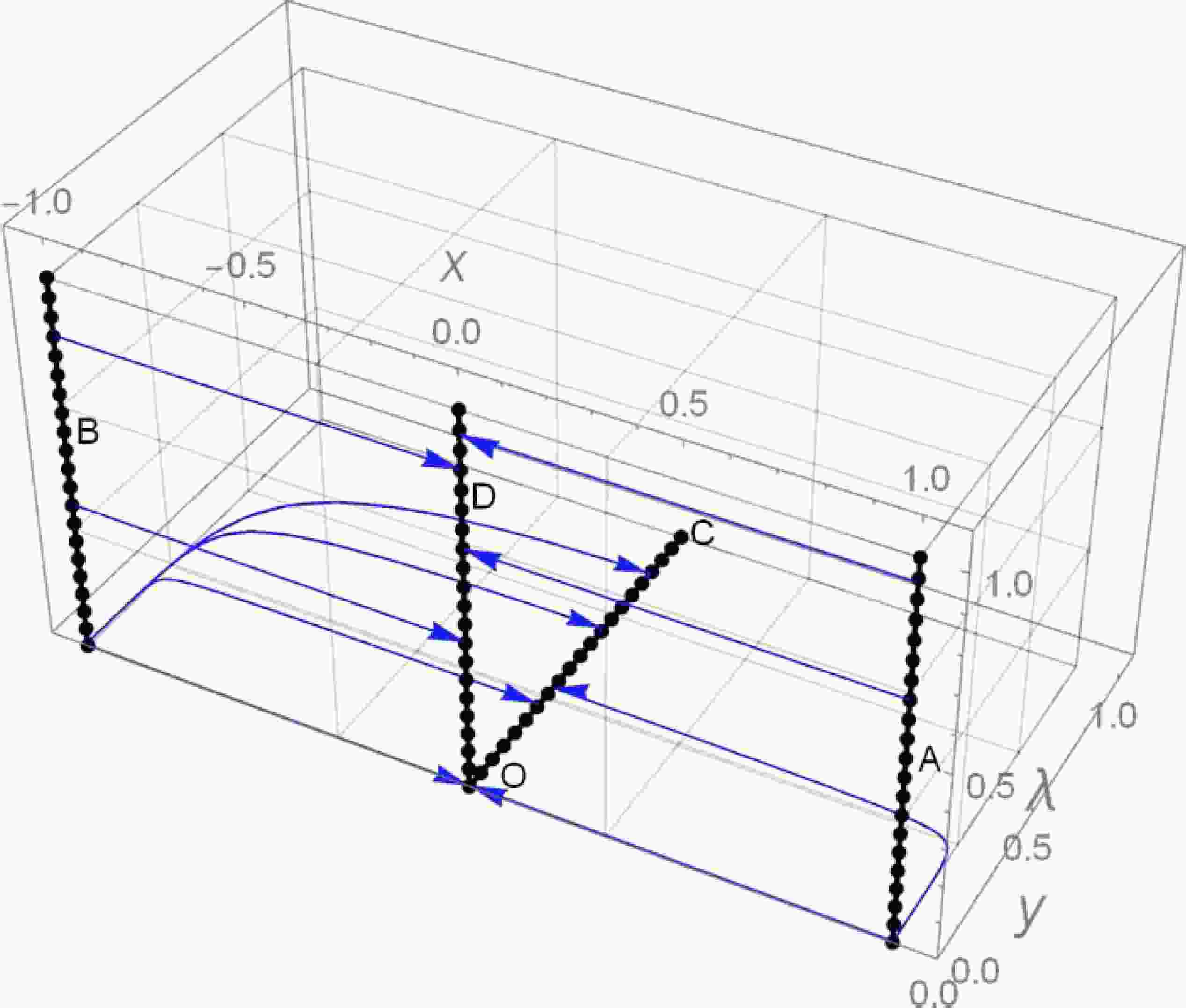
One of the main challenges of using string theory in cosmology directly is the so-called no-go theorem [51, 52], for wrapped products by compactification of the extra dimensions. According to the equations below the dynamical system equations, it is not closed for the generalized DBI field but is closed for an ordinary DBI. We also have compactified the phase space (λ axis) by Eq. (56). By compactification, we have drawn the three-dimensional (3D) phase space in Fig. 1.

Figure 1. (color online) 3D phase-space trajectories plotted for a set of solutions to the autonomous system presented in Eqs. (51)−(53) corresponding to the exponential potential.
Sen [11−13] predicted tachyon fields in both open and closed string theories. The open and closed string theories are presented in [9]. Even though for the closed string theory the tachyon fields are projected out in an open string, they remain. Even though we can use a spontaneous symmetry-breaking argument to get rid of tachyon modes, we can still fully explain the reason for their existence. In the bosonic string theory, if we use the Nambu-Goto action, it is almost impossible to quantize. To obtain meaningful quantization rules, we have to invoke the conformal invariant Polyakov action. Using the conformal field theory techniques, we can quantize such an action, which leads to the undesirable tachyon modes. Even though they violate the casualty, it can be shown that they are unstable. Thus, tachyon modes are typically expressed by a DBI Lagrangian,
$ \mathcal{L}_{\rm Tachyon}=V(\phi)\sqrt{1+\partial \phi^2}, $

(34) where
$ \partial\phi^2=\partial^{\mu}\phi\partial_{\mu}\phi $ ,$ V(\phi) $ is a potential function for the scalar field, and$ \partial^{\mu}\phi\partial_{\mu}\phi $ denotes the kinetic term for tachyon fields.Using the Lagrangian, we can find the field equation for the tachyon field from the Euler-Lagrangian equation:
$ \frac{\ddot{\phi}}{1-\dot{\phi}^2}+3H\dot{\phi}+\frac{V_{,\phi}}{V}=0 . $

(35) This is the modified Klein-Gordon equation for the DBI field.
The Friedmann equations (Eqs. (30) and (31)) become
$ 3H^2= \rho_{\rm DBI} + \rho_{de} , $

(36) $ \dot{H}=-\frac{1}{2} [\rho_{\rm DBI} + p_{\rm DBI}+\rho_{de}+p_{de}]. $

(37) Notably, for such cases, the energy density (
$\rho_{\rm DBI}$ ) and pressure ($p_{\rm DBI}$ ) are expressed by$ \rho_{\rm DBI}=\frac{V}{\sqrt{1-\dot{\phi}^2}} , $

(38) $ p_{\rm DBI}=-V\sqrt{1-\dot{\phi}^2}, $

(39) and thus the equation of state (
$\omega_{\rm DBI}$ ) is$ \omega_{\rm DBI}=\frac{p_{\rm DBI}}{\rho_{\rm DBI}}=\dot{\phi}^2-1. $

(40) We construct the autonomous dynamical system as follows. We can define the variables as
$ x=\dot{\phi} $ and$y= \dfrac{\sqrt{V}}{\sqrt{3}H}$ , and thus$ x^2=\dot{\phi}^2 $ ,$ y^2=\dfrac{V}{3H^2} $ , and$ s^2=\Omega_{de}=\dfrac{\rho_{de}}{3H^2} $ . Eq. (36) becomes$ s^2 = 1-\frac{y^2}{\sqrt{1-x^2}} . $

(41) To form the dynamical system, it is more convenient to take the “e-folding” timing defined as
$ N=\ln a $ . Thus, we obtain$\dfrac{\rm d}{{\rm d}t}=H\dfrac{\rm d}{{\rm d}N}.$ As
$ \dot{x}=\ddot{\phi} $ we can write$ x^{\prime}=\dfrac{\ddot{\phi}}{H} $ (where$ \prime $ denotes the derivative with respect to the “e-folding” time and$ \dot{} $ denotes the derivative with respect to the ordinary time). Utilizing this expressions in the Klein-Gordon equation for the DBI field in Eq. (35), we obtain$ \ddot{\phi}= (1-x^2)[\lambda V^{\frac{1}{2}}-3Hx]. $

(42) We defined the variable λ as
$ \lambda = -\dfrac{V_{,\phi}}{V^{\frac{3}{2}}} $ . Using Eq. (42) and$ y=\dfrac{\sqrt{V}}{\sqrt{3}H} $ in expression$ x^{\prime}=\dfrac{\ddot{\phi}}{H} $ , we obtain$ x^{\prime}=(x^2-1)(3x-\sqrt{3}\lambda y). $

(43) Further, by differentiating the variable y w.r.t e-folding time N, we obtain
$ y^{\prime}= -\frac{1}{2}y[\sqrt{3}\lambda xy+2\frac{\dot{H}}{H^2}] . $

(44) By utilizing Eqs. (32)−(33) and (38)−(39) in Eq. (37), we obtain
$ \frac{\dot{H}}{H^2}= \frac{3x^2y^2}{2\sqrt{1-x^2}[\Psi_Q+2Q\Psi_{QQ}-1]} . $

(45) Hence, Eq. (44) becomes
$ y^{\prime}= -\frac{1}{2}y[\sqrt{3}\lambda xy+ \frac{3x^2y^2}{\sqrt{1-x^2}[\Psi_Q+2Q\Psi_{QQ}-1]}] . $

(46) To obtain the closed form of variable λ, we define another quantity Γ as
$ \Gamma=\dfrac{VV_{,\phi\phi}}{V_{,\phi}} $ . By differentiating the variable λ w.r.t e-folding time N with the quantity Γ, we obtain$ \lambda^{\prime}= \sqrt{3} xy\lambda^2[\frac{3}{2}-\Gamma] . $

(47) In our analysis, we consider the cosmological model
$ f(Q)=-Q+\Psi(Q)=-Q+\alpha Q^n $ that has a high significance. A power-law correction to the STEGR leads to branches of solution applicable either to the early universe or to late-time cosmic acceleration. The model characterized by value$ n < 1 $ can describe the late-time cosmology, potentially influencing the emergence of dark energy, whereas the model characterized by value$ n > 1 $ can describe the early universe phenomenon [32]. Moreover, case$ \alpha=0 $ , i.e.,$ \Psi= 0 \Rightarrow f(Q)=-Q $ recovers the GR.Using
$ \Psi(Q)=\alpha Q^n $ , we obtain$(\Psi_Q+2Q\Psi_{QQ}- 1)= (2n-1)\alpha n Q^{n-1}-1$ .Moreover,
$ s^2=(-\dfrac{\Psi}{2}+Q\Psi_Q)\dfrac{1}{3H^2}= (2n-1)\alpha Q^{n-1} $ . Thus,$ [\Psi_Q+2Q\Psi_{QQ}-1]=ns^2-1 $ . Therefore, Eqs. (45) and (46) become$ \frac{\dot{H}}{H^2}= \frac{3x^2y^2}{[(n-1)\sqrt{1-x^2}-ny^2]}, $

(48) $ y^{\prime}= -\frac{1}{2}y \left[\sqrt{3}\lambda xy+ \frac{3x^2y^2}{[(n-1)\sqrt{1-x^2}-ny^2]}\right]. $

(49) -
The exponential potential in the DBI field can arise as, if we consider the dark matter with the phantom field (which can naturally arise from the string theory) and apply the fact in the present epoch, the dark matter energy density and phantom energy density are comparable (coincidence problem). This would lead to an exponential potential [24].
Therefore, we consider the following form of the exponential potential,
$ V(\phi)= V_0 {\rm e}^{-\beta \phi}. $

(50) For this choice of potential, we obtain
$\lambda=-\dfrac{V_{,\phi}}{V^{\frac{3}{2}}} = \dfrac{\beta}{\sqrt{V_0 {\rm e}^{-\beta\phi}}}$ and$ \Gamma=\dfrac{VV_{,\phi\phi}}{V_{,\phi}^2}=1 $ .Therefore, the complete autonomous form of dynamical equations (Eqs. (43), (47), and (49)) can be expressed as
$ x^{\prime}=(x^2-1)(3x-\sqrt{3}\lambda y) , $

(51) $ y^{\prime}= -\frac{1}{2}y[\sqrt{3}\lambda xy+ \frac{3x^2y^2}{[(n-1)\sqrt{1-x^2}-ny^2]}], $

(52) $ \lambda^{\prime}= \frac{\sqrt{3}}{2} xy\lambda^2. $

(53) Utilizing Eq. (48) and definition of deceleration parameter
$ q=-1-\dfrac{\dot{H}}{H^2} $ , we obtain the following expression corresponding to model parameter$ n=-1 $ ,$ q=-1-\frac{3x^2y^2}{-2\sqrt{1-x^2}+y^2} , $

(54) and the effective equation of state parameter is
$\begin{aligned}[b] \omega= &\omega_{\rm total}= \frac{p_{\rm eff}}{\rho_{\rm eff}} = \frac{p_{\rm DBI} + p_{de}}{\rho_{\rm DBI} + \rho_{de}}\\ = & -1-\frac{2\dot{H}}{3H^2} = -1-\frac{2x^2y^2}{-2\sqrt{1-x^2}+y^2} . \end{aligned}$

(55) We present the critical points and their behaviour (Table 1) for the autonomous system presented in Eqs. (51)−(53) corresponding to model parameter
$ n=-1 $ .Critical points
($ x_c,y_c,z_c $ )

Eigenvalues
($ \lambda_1 $ ,

$ \lambda_2 $ ,

$ \lambda_3 $ )

Nature of
critical pointq ω $ O(0,0,0) $ 

$ (-3,0,0) $ 

Nonhyperbolic(stable) $ -1 $ 

$ -1 $ 

$ A(1,0,\lambda) $ 

$ (6,0,0) $ 

Nonhyperbolic $ -1 $ 

$ -1 $ 

$ B(-1,0,\lambda) $ 

$ (6,0,0) $ 

Nonhyperbolic $ -1 $ 

$ -1 $ 

$ C(0,y,0) $ 

$ (-3,0,0) $ 

Nonhyperbolic(stable) $ -1 $ 

$ -1 $ 

$ D(0,0,\lambda) $ 

$ (-3,0,0) $ 

Nonhyperbolic(stable) $ -1 $ 

$ -1 $ 

Table 1. Critical points and their behaviour corresponding to model parameter
$ n=-1 $ and potential$V(\phi)= V_0 {\rm e}^{-\beta\phi}$ .As λ can have any value and is an even function (as the equation remains the same when
$ \lambda\rightarrow -\lambda $ ), we can consider the physical region of the given dynamical system as the positive half cylinder with infinite length from$ \lambda=0 $ to$ \lambda= +\infty $ . Hence, we compactify the variable by defining phase-space variable z [55],$ z=\frac{\lambda}{\lambda+1} \quad \text{or} \quad \lambda=\frac{z}{1-z}. $

(56) The evolutionary trajectories of the autonomous system presented in Eqs. (51)−(53) utilizing the above compactified variable are presented in Fig. 1.
The evolutionary profiles of scalar field density, dark energy density, deceleration, and equation of state parameter for the exponential potential are presented in Fig. 2.
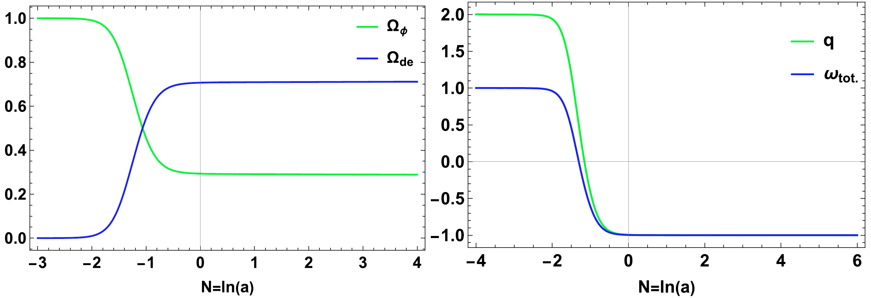
Figure 2. (color online) Evolutionary profiles of scalar field density, dark energy density, deceleration, and equation of state parameter for the exponential potential in the DBI scalar field.
We employed the entire plot in the
$ ln(a) $ axis (Fig. 2). The present value of the scale factor is set to$ a=1 $ , i.e.,$ N=\ln(1)=0 $ is the present time. Further,$ a < 1 $ , i.e.,$N={\rm ln}(a) < 0$ represents distant past, whereas$ a > 1 $ , i.e.,$N={\rm ln}(a) > 0$ represents distant future. -
For the critical point
$ A(1,0,\lambda) $ (obtained in Table 1), q exhibits an undefined form (see Eq. (54)). Thus, we are circumventing the problem by employing the appropriate limit of that fixed point.We first set
$ x=1-\epsilon_1 $ and$ y=\epsilon_2 $ in Eq. (48) (for the$ n=-1 $ case) where$ \epsilon_1,\epsilon_2>0 $ When we set$ \epsilon_1,\epsilon_2\rightarrow 0 $ we recover the original fixed points,$ \frac{\dot{H}}{H^2} =\frac{3(1-\epsilon_1)^2\epsilon_2^2}{\epsilon_2^2-2\sqrt{2\epsilon_1-\epsilon_1^2}} = \frac{3(1-\epsilon_1)^2}{1-2\sqrt{2\dfrac{\epsilon_1}{\epsilon_2^4}-\dfrac{\epsilon_1^2}{\epsilon_2^4}}}. $

(57) If we set the limit such that
$ \dfrac{\epsilon_1}{\epsilon_2^4}\rightarrow 1 $ , i.e.,$ \dfrac{1-x}{y^4}\rightarrow1 $ , as$ \dfrac{\epsilon_1^2}{\epsilon_2^4}\rightarrow0 $ we obtain$ \frac{\dot{H}}{H^2}=\frac{3}{1-2\sqrt{2}}\approx -1.64<-1 $

(58) Hence,
$ q=-1-\frac{\dot{H}}{H^2}\approx .64 . $

(59) Notably, for a matter-dominated universe (
$ a=t^{\frac{2}{3}} $ ),$ q=0.5 $ . Our limit along that particular trajectory when$ \dfrac{1-x}{y^4}\rightarrow1 $ leads to 0.64, which is quite consistent with the observation from the matter-dominated to the late-time acceleration phase.In the same limit,
$\omega=-1- \dfrac{2x^2y^2}{-2\sqrt{1-x^2}+y^2}\approx0.09 .$ The deceleration parameter has a crucial role to describe the expansion phase of the universe.
$ q < 0 $ depicts the accelerating behaviour whereas the transition from the acceleration phase to the deceleration phase corresponds to$ q \geq 0 $ . Thus,$ \begin{aligned}[b] q \geq 0 & \iff \frac{\dot{H}}{H^2} \leq -1 \iff \frac{3}{2\sqrt{2\dfrac{\epsilon_1}{\epsilon_2^4}-\dfrac{\epsilon_1^2}{\epsilon_2^4}}-1} \geq 1 \\ & \iff 2 \geq \sqrt{2\frac{\epsilon_1}{\epsilon_2^4}-\frac{\epsilon_1^2}{\epsilon_2^4}} \iff 2 \geq\frac{\epsilon_1}{\epsilon_2^4} \iff 2 \geq \frac{1-x}{y^4} . \end{aligned}$

(60) In the above equations, we used
$ x\rightarrow1 $ and$ y\rightarrow0 $ . The equality is valid when$ a\propto t $ .Similarly, criterion (60) leads to
$ \omega\geq -\dfrac{1}{3} $ . In addition, for an arbitrary n, criterion (60) for the transition from the acceleration phase to the deceleration phase becomes$ \dfrac{1-x}{y^4}\leq \dfrac{8}{(1-n)^2} $ .$ \dfrac{\dot{H}}{H^2}=\dfrac{3}{1-2\sqrt{2}} $ leads to$ a\propto t^{\frac{2\sqrt{2}-1}{3}}\approx t^{0.609} $ For a matter-dominated universe,$ a\propto t^{\frac{2}{3}}\approx t^{0.66} $ . Similarly, for the case of$ B(-1,0,\lambda) $ we can obtain identical expressions with similar expressions for q and ω, as the previous, with$ \epsilon_1=x+1 $ ($ x\geq-1 $ and near$ (-1,0,0) $ ).According to Fig. 3, we obtain a two-dimensional (2D) phase portrait for
$ x=1 $ , according to the corresponding eigenvalue for the critical point$ A(1,0,\lambda) $ . According to its nature, it is unstable, and$ q=-1 $ and$ \omega=-1 $ . Thus, it yields de Sitter-type solutions. There is a general theorem [51] and [52] that the type of potential with a well-defined minimum would always lead to de-Sitter-type solutions. We can verify this to some extent, as the assertion is valid even in a modified$ f(Q) $ gravity.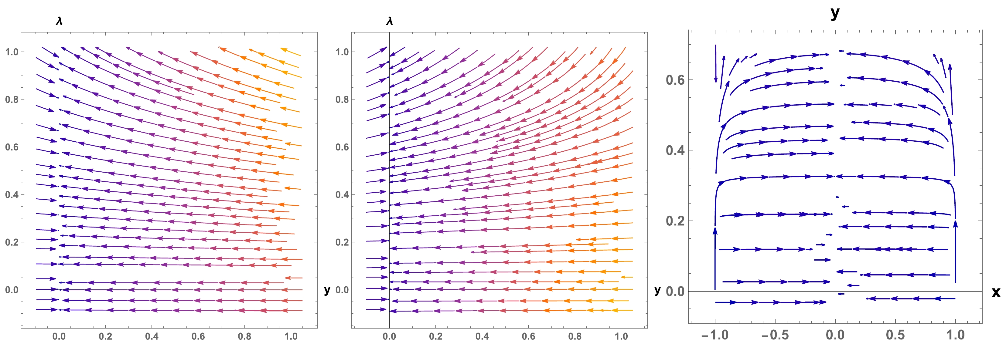
Figure 3. (color online) 2D phase portrait for the
$ x=1,-1 $ and$ xy $ planes. Even though the critical points are nonhyperbolic, we can employ particular limits to observe the matter-dominated to de Sitter transition. -
In this subsection, we use the power-law potential, as it most naturally provides global attractor solutions [20]. These solutions are stable under perturbation [22]. We assume the following form of power-law potential,
$ V(\phi)= V_0\phi^{-k} . $

(61) For this choice of potential, we obtain
$ \lambda=-\dfrac{V_{,\phi}}{V^{\frac{3}{2}}}= \dfrac{V_0k\phi^{-k-1}}{V_0\phi^{-k}(V_0\phi^{-k})^{\frac{1}{2}}}=\dfrac{k}{\sqrt{V_0}}\phi^{-1+\frac{k}{2}} $ .In particular, for
$ k=2 $ we obtain$ \lambda=\dfrac{2}{\sqrt{V_0}} $ .Further, the quantity Γ for the considered power-law potential becomes
$ \Gamma=\dfrac{VV_{,\phi\phi}}{V_{,\phi}^2}=\dfrac{k+1}{k} $ .Therefore, the complete autonomous form of dynamical equations (Eqs. (43), (47), and (49)) for the power-law potential becomes
$ x^{\prime}= (x^2-1)(3x-\sqrt{3}\lambda y), $

(62) $ y^{\prime}= -\frac{1}{2}y^2[\sqrt{3}\lambda xy+ \frac{3x^2y}{[(n-1)\sqrt{1-x^2}-ny^2]}], $

(63) $ \lambda^{\prime}= \frac{\sqrt{3}(k-2)}{2k} xy\lambda^2. $

(64) We present the critical points and their behaviour (Table 2) for the autonomous system presented in Eqs. (62)−(64) corresponding to the model parameter
$ n=-1 $ .Critical points
($ x_c,y_c,z_c $ )

Eigenvalues
($ \lambda_1 $ ,

$ \lambda_2 $ ,

$ \lambda_3 $ )

Nature of critical point q ω $ O'(0,0,\lambda) $ 

$ (-3,\sqrt{3}\lambda,0) $ 

Stable (NH) for $ \lambda<0 $ and

saddle for$ \lambda\geq0 $ 

$ -1 $ 

$ -1 $ 

$ A'(x,y,0) $ 

$ (-3,0,0) $ 

Nonhyperbolic (stable) $ -1 $ 

$ -1 $ 

$ B'(0,y,0) $ 

$ (-3,0,0) $ 

Nonhyperbolic (stable) $ -1 $ 

$ -1 $ 

Table 2. Critical points and their behaviour corresponding to model parameter
$ n=-1 $ and potential$ V(\phi)= V_0\phi^{-k} $ with$ k\neq2 $ .Notably, the dynamical equations presented for the power-law case in Eqs. (62)−(64) are identical to those presented for the exponential case in Eqs. (51)−(53). They differ only by a constant in the
$ \lambda' $ equation. Hence, the further analyses, i.e., evolutionary trajectories, are identical.In particular, for case
$ k=2 $ , the power-law case in Eqs. (62)−(64) differs from the exponential as it reduces to the following 2D dynamical system, as, for$ k=2 $ we obtain$ \lambda'=0 $ .$ x^{\prime}= (x^2-1)(3x-2\sqrt{3} y), $

(65) $ y^{\prime}= -\frac{1}{2}y^2[2\sqrt{3} xy+ \frac{3x^2y}{[(n-1)\sqrt{1-x^2}-ny^2]}]. $

(66) Notably, it is not surprising [22] that
$ k=2 $ indeed has a scale-invariant property, which forces a 2D dynamical system of equations. Here, without loss of generality, we assume$ V_0=1 $ and hence$ \lambda=\dfrac{2}{\sqrt{V_0}}=2 $ . We present the critical points and their behaviour (see Table 3) for the autonomous system presented in Eqs. (65) and (66) corresponding to model parameter$ n=-1 $ .Critical points $ (x_c,y_c) $ 

Nature of critical point q ω $ O''(0,0) $ 

Stable $ -1 $ 

$ -1 $ 

$ A''(0.806,0.698) $ 

Saddle $ 0.362 $ 

$ -0.092 $ 

Table 3. Critical points and their behaviour corresponding to model parameter
$ n=-1 $ with potential$ V(\phi)= V_0\phi^{-k} $ with$ k=2 $ and$ V_0=1 $ .The evolutionary trajectories of the autonomous system presented in Eqs. (65) and (66) are presented in Fig. 4.
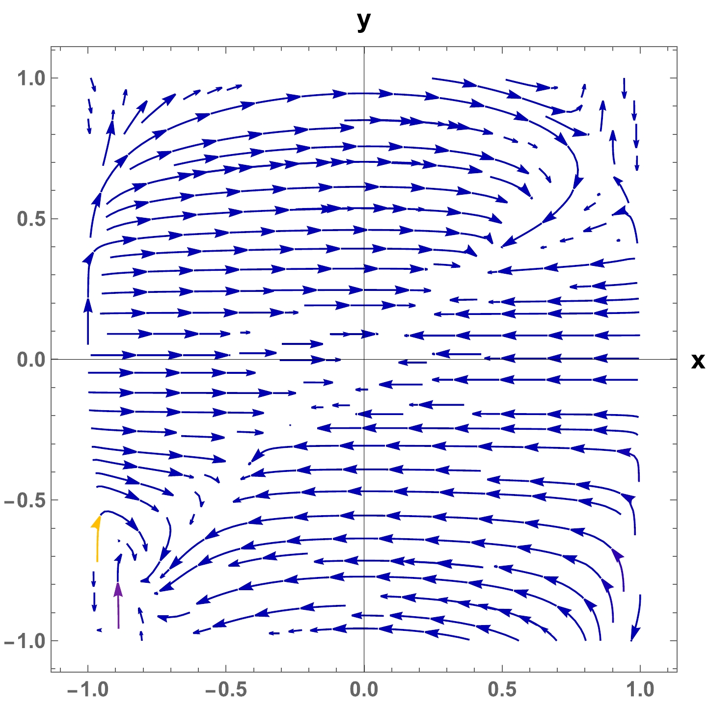
Figure 4. (color online) 2D phase portrait for a polynomial potential when
$ k=2 $ .According to the phase-space trajectories obtained in Fig. 4, the solution trajectory indicates the evolution from the saddle point
$ A'' $ representing a matter-like behavior to the stable point$ O'' $ representing the de-Sitter-type accelerated expansion phase, which is consistent with the analysis by Copeland et al. [20]. -
In this study, we investigated the DBI scalar field (the corresponding Lagrangian density is presented in Eq. (34)) and its effect on cosmology via a dynamical system analysis. The corresponding Klein-Gordon equation with Friedmann-like equations under the
$ f(Q) $ gravity formalism are presented in Eqs. (35), (36), and (37). For our analysis, we considered the cosmological model$f(Q) = -Q+\Psi(Q)=-Q+\alpha Q^n$ which is essentially a power-law correction to the STEGR case, which leads to branches of solution applicable either to the early universe or to late-time cosmic acceleration. The model characterized by$ n < 1 $ can describe late-time cosmology, potentially influencing the emergence of dark energy, whereas the model characterized by$ n > 1 $ can describe the early universe phenomenon [32]. We obtained a set of dynamical equations, i.e., Eqs. (43), (47), and (49), corresponding to the choice of our$ f(Q) $ function. Further, to obtain the closed form (i.e., autonomous form) of the system, we investigated two specific forms of the potential function, the exponential$ V(\phi)= V_0 {\rm e}^{-\beta \phi} $ and power-law$V(\phi)= V_0\phi^{-k}$ , which have been extensively studied in the GR context. We obtained the corresponding autonomous systems presented in Eqs. (51)−(53) and Eqs. (62)−(64). Their stability analysis is presented in Table 1 and Table 2. Moreover, the 3D phase-space trajectories of the autonomous system corresponding to the exponential potential are presented in Fig. 1. The behaviors of cosmological parameters such as deceleration, energy density, and effective equation of state parameter are presented in Fig. 2. The autonomous system equations presented for the power-law case in Eqs. (62)−(64) are identical to those presented for the exponential case in Eqs. (51)−(53); they differ only by a constant in the$ \lambda' $ equation. Hence, the further analyses, i.e., the evolutionary trajectories, are identical. Our fixed points have a late-time de-Sitter-type solution, as expected from the general theorem by Hao et al. [51] and Chingangbam et al. [52] about the sufficient condition for a de-Sitter-type solution. Further, we analyzed the fixed point$ (\pm1,0,\lambda) $ to show the transition from matter-dominated to de-Sitter-type solutions. In addition, we found the necessary and sufficient condition for the fixed points$ (\pm1,0,\lambda) $ to show a matter-dominated phase to de-Sitter phase,$ \dfrac{1-x}{y^4}\leq \dfrac{8}{(1-n)^2} $ (in the limit$ x\rightarrow 1 $ and$ y\rightarrow 0 $ ) corresponding to the generic model parameter, n. For the other fixed point$ (-1,0,\lambda) $ , we obtain similar results. In addition, we plotted the 2D phase portrait in Fig. 3 for the$ x=1,-1 $ and$ xy $ planes, which shows that, even though the critical points are nonhyperbolic, we can employ particular limits to observe the matter-dominated to de-Sitter transition. In addition, in the current time ($ N=0 $ ), we obtained$ q\approx -0.8 $ which is, to some extent, consistent with the present observed value (−0.55). The discrepancy in q occurs as there is no dark matter or ordinary matter in our calculations. Further, the power-law potential case for$ k=2 $ is different from the exponential, as$ k=2 $ yields$ \lambda^{\prime}=0 $ , which provides a 2D autonomous system presented in Eqs. (65) and (66). The corresponding stability analysis and phase portrait are presented in Table 3 and Fig. 4. Moreover, case$ k=2 $ matches those in the previous detailed studies [17, 20]. Thus, we successfully described the late-time epochs of the universe, particularly the de-Sitter expansion, and observed a transition epoch along with effects of the DBI field under the modified$ f(Q) $ cosmology. -
There are no new data associated with this article.
-
We thank the referee and editor for the valuable comments, which significantly improved our manuscript in terms of research quality and presentation.
Dynamical system analysis of Dirac-Born-Infeld scalar field cosmology in coincident f (Q) gravity
- Received Date: 2024-03-18
- Available Online: 2024-09-15
Abstract: In this article, we present a dynamical system analysis of a Dirac-Born-Infeld scalar field in a modified


 DownLoad: