Holographic timelike entanglement entropy from Rindler method

The Anti-de Sitter/Conformal Field Theory (AdS/CFT) correspondence [1−3] provides an interesting perspective on gravity and CFT: quantum gravity in a$(d+1)$-dimensional AdS spacetime is equivalent to a CFT on the d-dimensional boundary. Over the past two decades, an increasing number of evidences has supported this correspondence [4−9]. In particular, the holographic entanglement entropy [10−12] is one of the strongest evidences. In a quantum theory, if we divide the entire Hilbert space into two parts, A and B, the entanglement entropy $S_A$ is defined as the von Neumann entropy of the reduced density matrix $\rho_A$

where $\rho_A = \mathrm{Tr}_B(\rho)$; ρ denotes the density matrix for the whole system. In general, the calculation of entanglement entropy in CFT is not easy [13−15]. Fortunately, Ryu and Takayanagi proposed a method to calculate the entanglement entropy of a given region in CFT utilizing the AdS/CFT correspondence [10]. The Ryu-Takayanagi formula is elegant and simple. In short, the entanglement entropy of a region A in the boundary CFT can be expressed as the area of minimal surface $m_A$ in the bulk having the same boundary as A (denoted as $\partial A$),

where $G_{\rm N}$ is the Newton's constant.

Since the initial proposal by Ryu and Takayanagi, there have been several attempts to prove the Ryu-Takayanagi formula [16−18]. Among these, reference [17] was the first to use the conformal transformations to prove the formula for a spherical entanglement surface (i.e., $\partial A$). The basic idea of the proof is to utilize the conformal transformations to convert the calculation of the entanglement entropy into that of the thermal entropy in the CFT, which can then be mapped into the calculation of the black hole entropy in the gravitational dual according to the AdS/CFT correspondence. This method was later developed to derive the holographic entanglement entropy formula in other holographic theories [19−21] and is known as the "Rindler method".

There are many types of entanglement entropy [22]. Among them, pseudo-entropy is an interesting generalization of the entanglement entropy [23−26]. Its definition is similar to that of the entanglement entropy,

where $\tau_A$ is given by two pure states, $\left|\psi\right>$ and $\left|\varphi\right >$, as follows:

Although the expressions in Eqs. (3) and (1) are similar, pseudo-entropy is usually complex because Eq. (4) is not Hermitian. When $\left |\psi\right > = \left |\varphi\right >$, pseudo-entropy becomes ordinary entanglement entropy as defined in Eq. (1). When calculating the holographic entanglement entropy, the subregions considered are spacelike regions on the boundary. However, a recent study [27] has shown that the traditional spacelike entanglement entropy does not fully capture the entangling properties of CFTs, and timelike entanglement entropy needs to be introduced. Interestingly, a later study [28] found that the pseudo-entropy in dS/CFT is directly related to the timelike entanglement entropy in AdS/CFT. This timelike entanglement entropy is defined by analytically continuing a spacelike subregion into a timelike one. Furthermore, in [29], it is suggested that the time coordinate may emerge from the imaginary part of the timelike entanglement entropy or pseudo-entropy, generalizing the familiar idea that the space coordinate can emerge from the ordinary entanglement entropy [30−33]. Therefore, timelike entanglement entropy appears to be an important generalization of the ordinary entanglement entropy. Related work on the timelike entanglement entropy can be found in references [29, 34−40].

The timelike entanglement entropy is currently considered as a special pseudo-entropy. In the AdS/CFT framework, both the real and imaginary parts of pseudo-entropy have clear spacetime geometric interpretations [23]. Moreover, studies on quantum many-body systems suggest that pseudo-entropy can be used to detect quantum chaos in such systems [41] and to distinguish between different quantum phases [42]. Pseudo-entropy has been widely discussed in holographic duality, quantum field theory, quantum information, and quantum many-body systems [23, 24, 28, 43, 44]. However, the physical significance of timelike entanglement entropy is not yet well understood.

In this study, we used the Rindler method to re-examine the (holographic) timelike entanglement entropy in AdS₃/CFT₂ correspondence. Given that the introduction of the cut-off when calculating entanglement entropy using the replica trick [13−15] in field theory seems somewhat arbitrary, our treatment of the cut-off is different from those in previous studies [28, 29]. Specifically, our idea is that the entanglement entropy should be generally a function of the domain of dependence ${\cal{D}}$ and the cut-off of the subregion under consideration. When calculating entanglement entropy, a spacelike cut-off ε is always introduced. However, if we extend the entanglement entropy to timelike subregions, the cut-off naturally becomes timelike. This timelike cut-off $\varepsilon^{t}$ is used to replace the previous spacelike cut-off; consequently, the timelike entanglement entropy $S^{\left( t \right)}$ becomes

which is exactly the timelike entanglement entropy studied in references [28, 29].

This paper is organized as follows. In Sec. II, we briefly review the previous definition of timelike entanglement entropy and its holographic dual in AdS₃/CFT₂. In Sec. III, we first review how to calculate holographic entanglement entropy using the Rindler method. Then, we define timelike entanglement entropy and apply the Rindler method to obtain the gravitational dual of the timelike entanglement entropy. Finally, a discussion and conclusions are provided in Sec. IV.

Let us consider a spacelike interval $A = [(t_1,x_1), (t_2,x_2)]$ in a $(1+1)$ dimensional Minkowski space (with the signature of the metric as $(-1,+1)$), and let us define

Using the replica trick [13−15], one can obtain the entanglement entropy of the subregion A as

where c is the central charge of the CFT and ε is a UV cut-off. Now let us suppose that the entanglement entropy formula also applies to the timelike interval, which defines the timelike entanglement entropy [29]. Thus, $X^2_0-T^2_0<0$. Consequently, we obtain the timelike entanglement entropy:

The definition of timelike entanglement entropy can also be extended to finite size CFT and finite temperature CFT, respectively,

where R is the total length of the finite system, $\Delta t$ is the difference between the time coordinates of the endpoints of the considered interval, $\Delta \phi$ and $\Delta x$ are the differences between the coordinates in the spatial direction of the considered interval, and β is the inverse of the finite temperature.

In terms of the AdS₃/CFT₂ correspondence, one can define the metric of the AdS₃ spacetime in Poincaré coordinate as (the AdS radius is set to $\ell_{\rm{AdS}} = 1$)

In the boundary CFT₂, we consider a timelike interval of length $T_0$ with fixed spatial coordinates. In this case, there are no spacelike geodesics which can directly connect the boundaries of the timelike interval in the CFT. However, this timelike interval can be connected by two spacelike geodesics and one timelike geodesic in the bulk of AdS₃, as shown in Fig. 1. The spacelike geodesics (in blue) connect the endpoints of the interval to null infinity, while the timelike geodesic (in purple) connects the endpoints of the two spacelike curves at null infinity [28]. Therefore, the spacelike geodesics are given by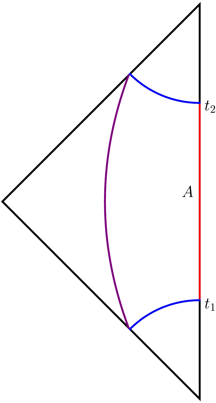

Figure 1.  (color online) Penrose diagrams of the geodesics connecting the boundary subregions, where the boundary subregion A is represented by the red line segment. The blue curves represent the spacelike geodesics, while the purple curve represents the timelike geodesic.

and the form of the timelike geodesic is

where $t_0$ and $z_0$ are two constants determined by the endpoint positions of the spacelike geodesic at null infinity. The final results indicate that two spacelike geodesics contribute to the real part of the timelike entanglement entropy, while the timelike geodesic corresponds to the imaginary part of the timelike entanglement entropy.

It is worth noting that the appearance of the imaginary part in the definition of timelike entanglement entropy seems strange, regardless of how you examine it. There seems to be an analytic continuation to make the holographic entanglement entropy applicable to timelike intervals, but the cut-off is still that corresponding to spacelike intervals. Therefore, an imaginary part appears. Thus, there can naturally be an equivalent definition, where the interval is still a spacelike interval, but the cut-off is taken in the timelike interval. This is precisely the idea behind another approach for defining timelike entanglement entropy in reference [29]. (We briefly review this definition in Appendix A.)

In this section, we describe an alternative perspective on timelike entanglement entropy based on the Rindler method. For the convenience of the reader and subsequent narrative, we first briefly review how to compute the holographic entanglement entropy in AdS₃/CFT₂ using the Rindler method. Interested readers can refer to references [17, 19−21, 45−47].

Consider a spatial interval ${\cal{I}}$ whose domain of dependence in a two-dimensional Minkowski spacetime is given by

in which we have set $u = x+t$ and $v = x-t$. The key to the Rindler method is to find a Rindler transformation that maps ${\cal{D}}$ to an infinitely large region ${\cal{B}}$. This is a conformal transformation that maps the vacuum state in ${\cal{D}}$ to ${\cal{B}}$ and correspondingly maps the entanglement entropy of ${\cal{I}}$ to the thermal entropy in ${\cal{B}}$. For a two-dimensional CFT, the Rindler transformation is

This transformation implies that the thermal circle in ${\cal{B}}$ is

Consequently, the thermal entropy in ${\cal{B}}$ gives rise to the desired entanglement entropy.

According to the AdS/CFT correspondence, the computation of thermal entropy can be transformed into the computation of black hole entropy in the gravitational dual, which can be obtained by applying the Rindler transformation in the bulk:

where $u, v$, and z are coordinates in the Poincaré AdS₃ metric ${\rm d} s^{2} = \dfrac{1}{z^{2}}\left({\rm d} z^{2} + {\rm d} u {\rm d} v\right)$. After this transformation, the new metric becomes

Its event horizon is located at

Substituting Eq. (21) into Eq. (17) yields

or

Combining Eqs. (22) and (23) yields the RT/HRT surface:

Therefore, the final result of the entanglement entropy is

where $\varepsilon_u$ and $\varepsilon_v$ are introduced as cut-offs in the u and v directions, as shown in Fig. 2.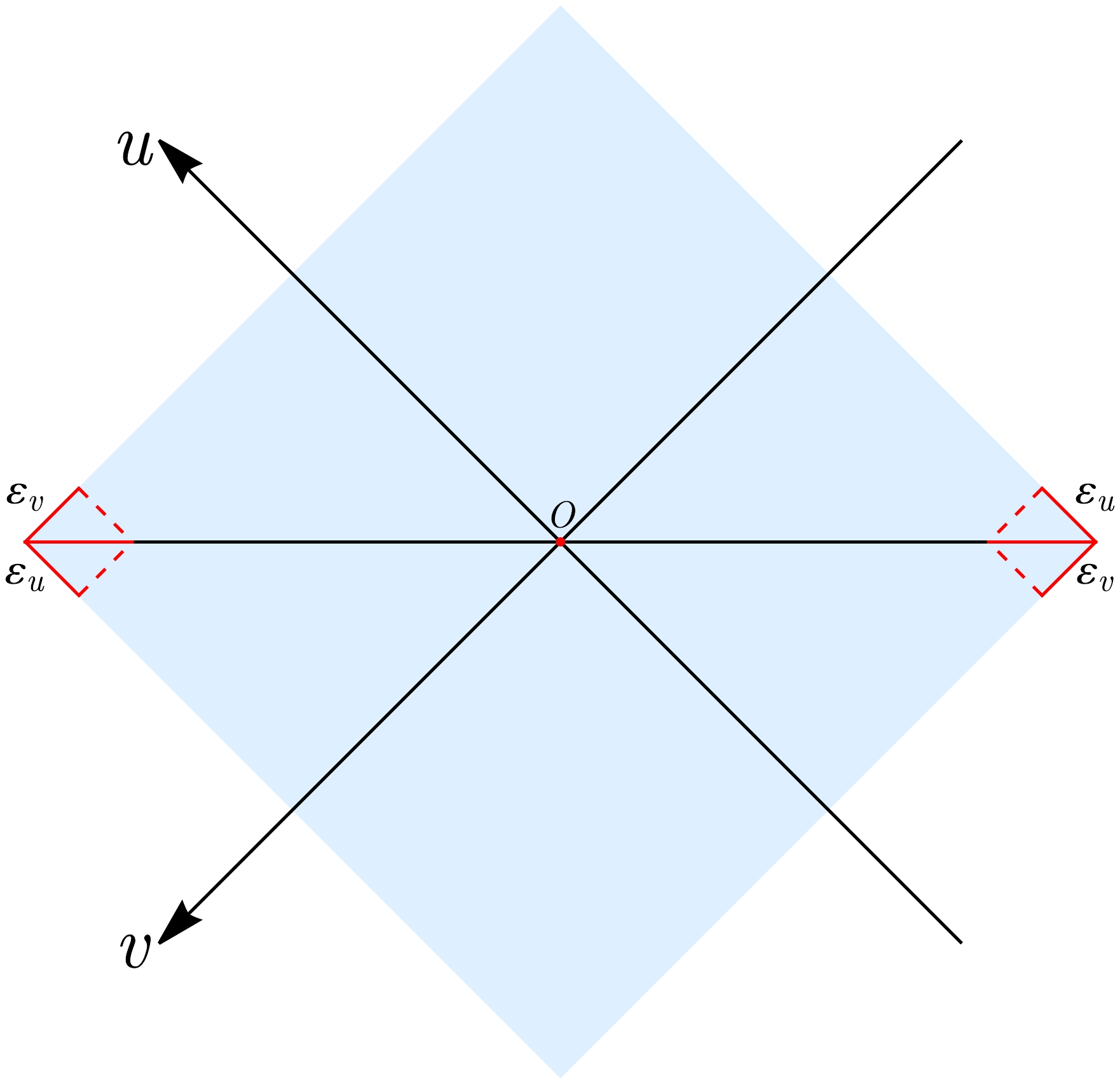

Figure 2.  (color online) A schematic diagram of a spatial interval (horizontal line) and its domain of dependence (blue shape), with cut-offs $\varepsilon_{u},\varepsilon_{v}$ marked in the diagram.

More generally, we can consider subsystems (i.e., spacelike curves with a domain of dependence of ${\cal{D}}$) with different truncations at the left ($\varepsilon_{u1},\varepsilon_{v1}$) and right ($\varepsilon_{u2},\varepsilon_{v2}$) ends. In this case, the entanglement entropy becomes

Given that $l_{u}$ and $l_{v}$ are related to the domain of dependence of the subsystem, the entanglement entropy can be eventually obtained once the subsystem is given and the truncations are chosen.

As mentioned above, Eqs. (25) and (26) can be regarded as functions that depend on the domain of dependence and cut-off, where the domain of dependence is characterized by $l_{u}l_{v}$. Next, we elaborate on the concept of entanglement entropy to be applicable not only to spacelike subregions but also to timelike subregions. A natural idea is that the "entanglement entropy" of a timelike region is also related to a spacetime subregion and cut-offs. We expect that this spacetime subregion remains the causal domain of some spacelike interval. The current issue is how to establish a connection between a spacelike interval and a timelike interval. Below, we proceed to accomplish this task.

Let us suppose there is a spacelike curve ${\cal{I}}_s$ with parametric equations:

where s is the parameter. Then, we can define a timelike curve ${\cal{I}}_t$ as

which is called the dual to ${\cal{I}}_s$. From Eq. (28) we can clearly see that ${\cal{I}}_s$ and ${\cal{I}}_t$ are symmetric to each other, with the u axis as the symmetry axis. Therefore, ${\cal{I}}_s$ connects the left and right endpoints of the domain of dependence, while ${\cal{I}}_t$ connects the upper and lower endpoints of the domain of dependence. Figure 3 provides an intuitive illustration of this setup.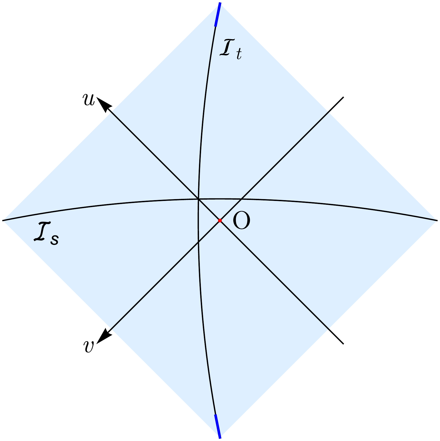

Figure 3.  (color online) Illustration of the spacelike curve ${\cal{I}}_s$ and its dual timelike curve ${\cal{I}}_t$. The cut-offs of ${\cal{I}}_{t}$ are marked by the blue line segment.

Next, we define the "cut-offs" $\varepsilon_u$ and $\varepsilon_v$ on the spacelike curve with $s_1$ and $s_2$ as two parameters:

where $s_{2}-s_{1}\rightarrow0^{+}$. To clarify this, we analyze a specific example. Let us suppose a spacelike curve defined as

After the cut-off, its regulated version is

where ε is a positive infinitesimal parameter whose relationships with $\varepsilon_u$ and $\varepsilon_v$ are

Therefore, we can obtain the entanglement entropy for the above subregion, which is exactly given by Eq. (25).

It is evident that for the dual timelike versions of Eqs. (30) and (31), the truncations are

in which the superscript t denotes "timelike". This relationship holds for any two dual curves. If we generalize the entanglement entropy in a way that Eq. (25), which holds for the spacelike subregions, also holds for the timelike subregions, then the entanglement entropy of the timelike subregion ${\cal{I}}_t$, which is dual to the spacelike subregion ${\cal{I}}_s$, becomes

It is evident that the entanglement entropy of the resulting timelike interval only differs from the entanglement entropy of the corresponding spacelike interval by an additional term of ${\rm i}\pi c/6$. When $l_{u} = l_{v}$, Eq. (34) is exactly the timelike entanglement entropy introduced in references [28, 29, 36]. More generally, we can extend Eq. (26) to the entanglement entropy of timelike subregions:

Compared to references [28, 29, 36], the formula for timelike entanglement entropy derived here has a broader applicability. It is applicable to any timelike interval, not limited to pure null intervals. Our method for defining timelike entanglement entropy can be directly applied to the finite size CFT and finite temperature CFT, with an extra ${\rm i}\pi c/6$ added, similar to Eq. (35). We did not elaborate on this in this study.

A question arising is whether the Rindler method can also be applied to derive the gravitational dual of the timelike entanglement entropy $S_{\mathrm{TEE}}$. The formal expression of Eq. (34) is

i.e., the timelike entanglement entropy is equal to the sum of the thermal entropy $S_{\mathrm{thermal}}$ undergoing a Rindler transformation and the constant ${\rm i}\pi c/6$. However, Sec. III.A shows that the thermal entropy here corresponds to the black hole entropy, and the black hole horizon corresponds to the RT/HRT surface. Similar to the usual calculation of holographic entanglement entropy, the black hole entropy can only provide a real area [17]; it cannot provide an imaginary part. Therefore, it seems that this method does not directly provide a gravitational dual for timelike entanglement entropy.

Nevertheless, an alternative solution is to modify the Rindler transformation so that the black hole horizon precisely corresponds to the two spacelike geodesics in the gravitational dual of timelike entanglement entropy. Mathematically speaking, there is no difference between the negative sign appearing on $\varepsilon_v$ or $l_v$ in Eq. (34), that is,

Following this approach, we can replace all $l_v$ in the Rindler method with $-l_v$. Therefore, the previous Rindler transformation defined by Eqs. (17)−(19) in the bulk becomes

Interestingly, this new transformation also turns the Poincaré AdS₃ metric into Eq. (20). Correspondingly, in the boundary conformal field theory, this transformation becomes

This transformation can map the domain of dependence ${\cal{D}}$ to ${\cal{B}}$ as well. Therefore, the thermal entropy in ${\cal{B}}$ remains unchanged and can also be given by the horizon entropy expressed by Eq. (20). Then, we substitute the horizon $z^\prime_h = 1$ into Eq. (38), obtaining

or

These are exactly the two spacelike geodesics in the gravitational duality of the timelike entanglement entropy mentioned in references [28, 29, 36]. To examine this more closely, we set $l_{u} = l_{v} = l$; then, Eqs. (42) and (43) become

and

Note that $u = x+t$ and $v = x-t$; thus, we have

If we change the notation to be $l = T_{0}$, then Eq. (46) describes precisely the spacelike geodesics in Eq. (12), and their areas are related to the real part of the timelike entanglement entropy. By connecting the endpoints of the two spacelike geodesics at null infinity with timelike geodesics, we can finally obtain the complete form of the holographic timelike entanglement entropy, i.e., $S_{\rm TEE} = S_{\rm thermal}+ {\rm i}\pi c/6$.

In this study, we re-examined the holographic entanglement entropy in AdS₃/CFT₂. For a Lorentz invariant theory, we assumed that the entanglement entropy should be a function of the domain of dependence of the region under consideration. By generalizing the concept of cut-off or defining a cut-off that is applicable to both spacelike and timelike regions, we rei-ntroduced the timelike entanglement entropy. We found that the timelike entanglement entropy is the thermal entropy of the CFT after applying the Rindler transformation plus the constant ${\rm i}\pi c/6$. Moreover, we obtained the gravitational dual of the timelike entanglement entropy, which is consistent with previous results.

There are some interesting issues which need further investigation. For instance, in the usual Rindler approach, the Rindler transformation is a symmetric transformation; for instance, in conformal field theory, it is a conformal transformation. This symmetric transformation induces a unitary operator U in Hilbert space that relates the density matrix ρ of the vacuum state in the original u, v coordinate system to the thermal density matrix $\rho^\prime$ in the $u^\prime$, $v^\prime$ coordinate system,

Given that the unitary transformation does not change the von Neumann entropy, the entanglement entropy of the vacuum state is equal to the thermal entropy of the transformed thermal state [17].

If we assume that the timelike entanglement entropy is also the von Neumann entropy of some "density matrix", given that the current Rindler transformation expressed by Eq. (41) is no longer a conformal transformation, we have reasons to believe that the timelike entanglement entropy is related to the "transformed thermal entropy", but not exactly equal to it. This is in perfect agreement with Eq. (36) and also explains why we were unable to directly obtain the timelike geodesics given by Eq. (13) connecting the two spacelike geodesics from the Rindler method. Moreover, one can consider the new "Rindler transformation" to be composed of a transformation

and the original Rindler transformation

The transformation expressed by Eq. (48) makes ${\rm d}s^2\rightarrow -{\rm d}s^2$. Such a transformation turns timelike curves into spacelike curves and vice versa. For convenience, this paper refers to it as "dual transformation". Although the properties of this dual transformation remain unknown, we can naively conjecture that under the dual transformation, the entanglement entropy remains unchanged up to a constant ${\rm i} \pi c/6$. (Further discussion can be found in Appendix B.)

Holographic entanglement entropy also leads to the interesting idea that the spatial coordinates of AdS come from quantum entanglement [31, 48]. It is natural to hypothesize whether the time coordinate also comes from quantum entanglement. Timelike entanglement entropy is likely to be a quantity related to the emergence of the time coordinate, although its physical meaning is not yet clear [29]. However, it opens a new window for generalizing entanglement entropy and deserves further study.

Consider a free scalar field on a cylinder with mass m. The space and time coordinates are denoted by x and t, respectively. Assuming that the spatial circle is $x\sim x+R$, we can easily express the action of the scalar field as

To define the timelike entanglement entropy, we treat t as the spatial direction and x as the Euclidean time. It can be considered that the spacetime has been rotated by 90 degrees. Then, the "timelike Hamiltonian" H is

where

Then, the partition function is

We introduce the rescaled Hamiltonian $\tilde{H} = {\rm i} H$, which takes the conventional form with a minus sign for the mass term:

Eq. (A4) can be rewritten as

$1/\beta_s$ is the temperature of the cylinder after spacetime rotation. A spacelike region A on this cylinder corresponds to a timelike region on the cylinder before rotation. We can obtain the timelike entanglement entropy by making the following substitution to the usual entanglement entropy formula:

For two-dimentional CFT, the entanglement entropy for the thermal state at temperature $1/\beta_s$ is

where X is the length of the spatial interval A;$\tilde{\epsilon}$ is the cut-off defined for $\tilde{H}$, while $\varepsilon = {\rm i}\tilde{\epsilon}$ is defined for the Hamiltonian H we are interested in. By making the substitutions in Eq. (A7) as mentioned earlier and setting $X = T_0$, we obtain the timelike entanglement entropy:

If we set $R\rightarrow\infty$, we obtain

This is precisely Eq. (8) in the case of a pure timelike interval.

To express our ideas more clearly, we would like to provide some explanations on the origins of ${\rm i}\pi c/6$. In the preceding text, we mentioned the following coordinate transformation:

This transformation is equivalent to swapping the spacetime coordinates:

Then we have

and

Let us suppose ${\rm d}s^{2}$ and ${\rm d}s^{\prime\prime 2}$ describe the geometries M and $M^{\prime\prime}$, respectively. Then, a timelike curve in M corresponds to a spatial curve in $M^{\prime\prime}$. In $M^{\prime\prime}$, we can use an ordinary Rindler transformation to obtain the entanglement entropy of the spatial curve, which has the following form:

in which the cut-offs must be calculated by the spacetime interval. We aim to define the timelike entanglement entropy in M through the entanglement entropy of $M^{\prime\prime}$ by directly replacing the domain of dependence and cut-offs in S. Interestingly, the corresponding domains of dependence on M and $M^{\prime\prime}$ are identical, but the cut-offs differ, leading to a term ${\rm i}c\pi/6$ in the timelike entanglement entropy.