A Numerical Study on Gauge Symmetry of Electroweak Amplitudes

The gauge cancellation of electroweak (EW) scattering amplitudes in the standard model (SM) [1−3] has been both a theoretical problem hindering physical analysis and a practical problem in numerical calculations. In recent years, a new framework of computing EW amplitudes based on Goldstone equivalence was proposed and implemented in the software package HELAS [4]. The main ingredients of this framework are: 1) taking Goldstone equivalence [5−7], so that the polarization vector of a massive vector boson has no $ k^\mu $ term, instead is composed of its Goldstone component and a remnant gauge term; 2) combining the gauge components and their Goldstone component of fields or polarization vectors into single 5-component objects at the level of polarization vectors, propagators, and vertices; 3) imposing a special light-cone gauge defined by the gauge direction $ n^\mu=(1,-{\vec k}/{|\vec k|}) $, dubbed the Feynman diagram gauge [4] or Goldstone equivalence gauge [8]. It has been demonstrated in Ref. [4] with many examples that EW amplitudes in this new scheme do not have gauge cancellation, thereby solving a long-standing problem. Further studies on this topic can be found in Refs. [9−15]. Earlier but incomplete treatment of the 5-component formalism can be found in [16−18].

The new framework in Ref. [4] is essentially a reorganization and combination of "pieces" from existing Feynman rules. Although ideal to be combined with the Feynman diagram gauge, it can also be applied to other gauges, such as the Feynman gauge and others. Therefore, it is necessary to distinguish the 5-component framework from any specific choice of gauge. Additionally, since the framework relies on the Goldstone equivalence theorem [5−7] in an essential way, it is appropriate to refer to it as the Goldstone equivalence (GE) representation of Feynman rules, as we will do from now on. Correspondingly, the standard Feynman rules will be called the gauge representation, as they exclusively treat the physical content of massive vector bosons as quanta of gauge fields.

Although the absence of gauge cancellation is crucial for practical applications, it is not the only important property of the GE representation of EW Feynman rules. Another intriguing property is that the GE representation directly imprints gauge symmetry at the level of amplitudes, as expressed by the massive Ward identity (MWI), which is named in analogue to its massless counterpart. Specifically, for a scattering amplitude $ \varepsilon^{\mu(*)}(k) {\cal{M}}_\mu $ involving an external vector boson V with mass $ m_V $ and 4-momentum $ k^\mu $, the MWI reads [5−7, 19]

where the $ - $ ($ + $) sign corresponds to the case that the vector boson is in the initial (final) state, and $ {\cal{M}}(\varphi) $ represents the amplitude obtained by replacing the vector boson with the corresponding Goldstone boson φ. The MWI (1) is a fundamental identity for a spontaneously broken gauge theory, e.g., the EW gauge theory. The main goal of this work is to study gauge symmetry of EW amplitudes using the numerical tool HELAS [4, 20, 21].

Similar to the Ward identity in gauge theories with massless gauge bosons, the MWI guarantees precise relations among different diagrams of an amplitude, which further imply exact relations among different vertices, or equivalently, different couplings within the same theory. Taking the example of $ W^+ W^- \rightarrow W^+ W^- $ with the helicity combination of $ {\rm{TTTT}} $, where $ {\rm{T}} $ represents a transverse polarization, the amplitude includes three vertices $ WWZ $, $ WWA $, and $ WWWW $ with couplings $ g_{WWZ} $, $ g_{WWA} $, and $ g_{WWWW} $. The Ward identity requires

Conversely, any deviation from this relation would result in violations of the gauge symmetry and the Ward identity. When the helicity combination involves longitudinal components, the precise relations the MWI brings about not only involve couplings of gauge bosons, but also those of Goldstone bosons and the Higgs boson. Thus, the structure of gauge symmetry is much richer in massive amplitudes, on which we will devote much space to study. Moreover, the gauge symmetry and the MWI are not limited to the SM but can also be applied to other theories. One theory of particular interests is the standard model effective field theory (SMEFT) [22−27], which is a direct extension of the SM.

The remaining of the paper is organized in the following way. In Section II, we provide a brief introduction to the GE representation of EW interactions, emphasizing on the relations among different couplings and parameters. In Section III, we directly test the EW gauge symmetry with the MWI (1) across multiple processes and helicity combinations. In Section VI, we examine the EW gauge symmetry through anomalous couplings, including both within individual vertices and among multiple vertices. Finally in Section V, we study the connection between anomalous couplings (Higgs self-couplings and Yukawa couplings) and certain SMEFT operators using the MWI. We will demonstrate that when the anomalous couplings are adjusted according to the SMEFT operators, the MWI is satisfied, ensuring gauge invariance and self-consistency of the theory.

In this section, we describe key ingredients of the GE representation, including polarization vectors, gauge choice, propagator, vertices, and Feynman rules.

The central identity for our program is the massive Ward identity (1), which essentially states the equivalence between the $ k^\mu $ terms in gauge fields and the corresponding Goldstone fields. Moreover, the longitudinal polarization vector of a massive vector boson V with 4-momentum $ k^\mu $ can be decomposed into

with $ n^\mu=(1, -{\vec k}/{|\vec k|}) $ and the subscript $ {\rm{L}} $ representing a longitudinal polarization. We can eliminate the $ k^\mu $ term in $ \epsilon_{\rm{L}}^\mu(k) $ by using the MWI, resulting in the amplitude with a longitudinal vector boson to become

where the MWI (1) is used in the second step.

The generalization to multiple vector bosons is straightforward, but it leads to an excessive number of terms, making calculations cumbersome. To address this issue, we define 5-component longitudinal polarization vectors in the GE representation by combining the gauge boson wave function and the Goldstone boson "wave function" as

with $ \mu = 0,1,2,3 $ and $ M = 0,1,2,3,4 $. In addition, the 5-component transverse polarization vectors are defined as $ \epsilon^M_\pm(k) = \big(\epsilon^\mu_\pm(k),\; 0\big) $. Then, the MWI (1) can be rewritten as

with $ {\cal{M}}^M \equiv ({\cal{M}}^\mu, {\cal{M}}(\varphi)) $ and the 5-component "momentum" $ k^M \equiv (k^\mu, -im_V) $. The 5-dimensional "metric" for index contraction is $ g_{MN} \equiv \operatorname{diag}(+1, -1, -1, -1, -1) $. The spin sum of the polarization vectors becomes

with $ g^{MN} = \operatorname{diag}(+1, -1, -1, -1, -1) $ and $ n^M \equiv (n^\mu, 0) $. Writing the gauge and Goldstone components separately, Eq. (7) becomes

The mixing between gauge and Goldstone degrees of freedom is manifest here. When $ m_V\rightarrow 0 $, they decouple from each other.

Because of the MWI (6), we can go further to state that the longitudinal polarization vector can be equivalently defined by an arbitrary shift:

gives the same amplitudes for any value of λ. Choosing $ \lambda = 1 $ yields $ \epsilon_{\rm{L}}^M(k,1) = (\epsilon_{\rm{L}}^\mu(k), 0) $, which corresponds to the conventional case using Eq. (3). We will refer to the case of $ \lambda =1 $ as the gauge form of the longitudinal polarization. The case of $ \lambda =0 $ corresponds to Eq. (5), which we will call the GE form.

The 5-component formalism can also be naturally derived from the Lagrangian, which includes a term $ m_V V_\mu \partial^\mu\varphi $ that mixes the gauge field with the Goldstone field after gauge symmetry breaking [4]. Therefore, it is natural to combine gauge and Goldstone components into one 5-component object.

The GE representation, implemented through the 5-component formalism, is compatible with any gauge except the unitary gauge, which eliminates Goldstone bosons from the Feynman rules. In the $ R_\xi $ gauges, the gauge-fixing Lagrangian term $ -(\partial^\mu V_\mu -m_V \varphi)^2/(2\xi) $ is introduced to cancel the gauge-Goldstone mixing term. This results in the propagator for a massive vector boson in the 5-component formalism taking the form of

Setting $ \xi = 1 $ yields the Feynman gauge.

To completely eliminate the $ k^\mu $ terms, we can choose the gauge condition $ n^\mu(x) V_\mu(x) =0 $, where $ n^\mu(x) $ is the Fourier transformation of $ n^\mu(k) = (1,-{\vec{k}}/{|\vec{k}|}) $, by adding the Lagrangian term $ -[n^\mu(x) V_\mu(x)]^2/(2\alpha) $. Its specific form is irrelevant here. Applying to a massive gauge theory, the 5-dimensional vector boson propagator becomes

The numerator of the gauge independent part is precisely the spin sum of polarization vectors in Eq. (7) for an on-shell momentum. Taking $ \alpha \to 0 $, we obtain the polarization vector in Eq. (9) with $ \lambda=0 $. This is known as the Goldstone equivalence gauge or the Feynman diagram gauge [4].

With the polarization vectors and the propagator expressed in the 5-component formalism, it is natural to extend this framework to vertices involving massive vector bosons. To reflect this property, we introduce a double-line notation by overlapping a wavy line with a dashed line to represent the massive vector boson in Feynman rules: the wavy line represents the gauge components, while the dashed line represents the Goldstone component. As examples of this double-line notation, we illustrate the decomposition of the vector boson propagator in Fig. 1 and that of the $ WWh $ vertex in Fig. 2.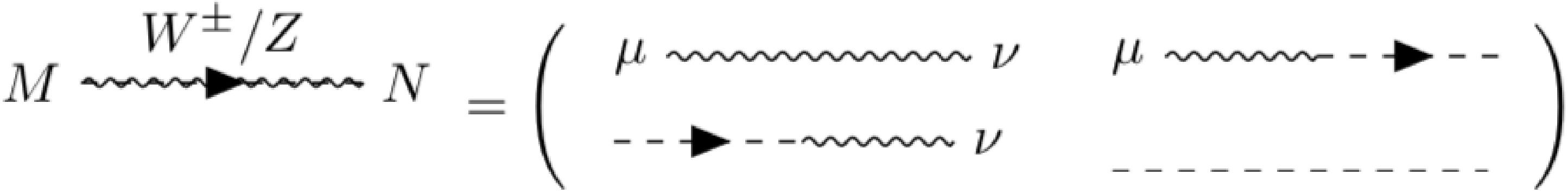

Figure 1.  5-component vector boson propagator in the double-line notation.

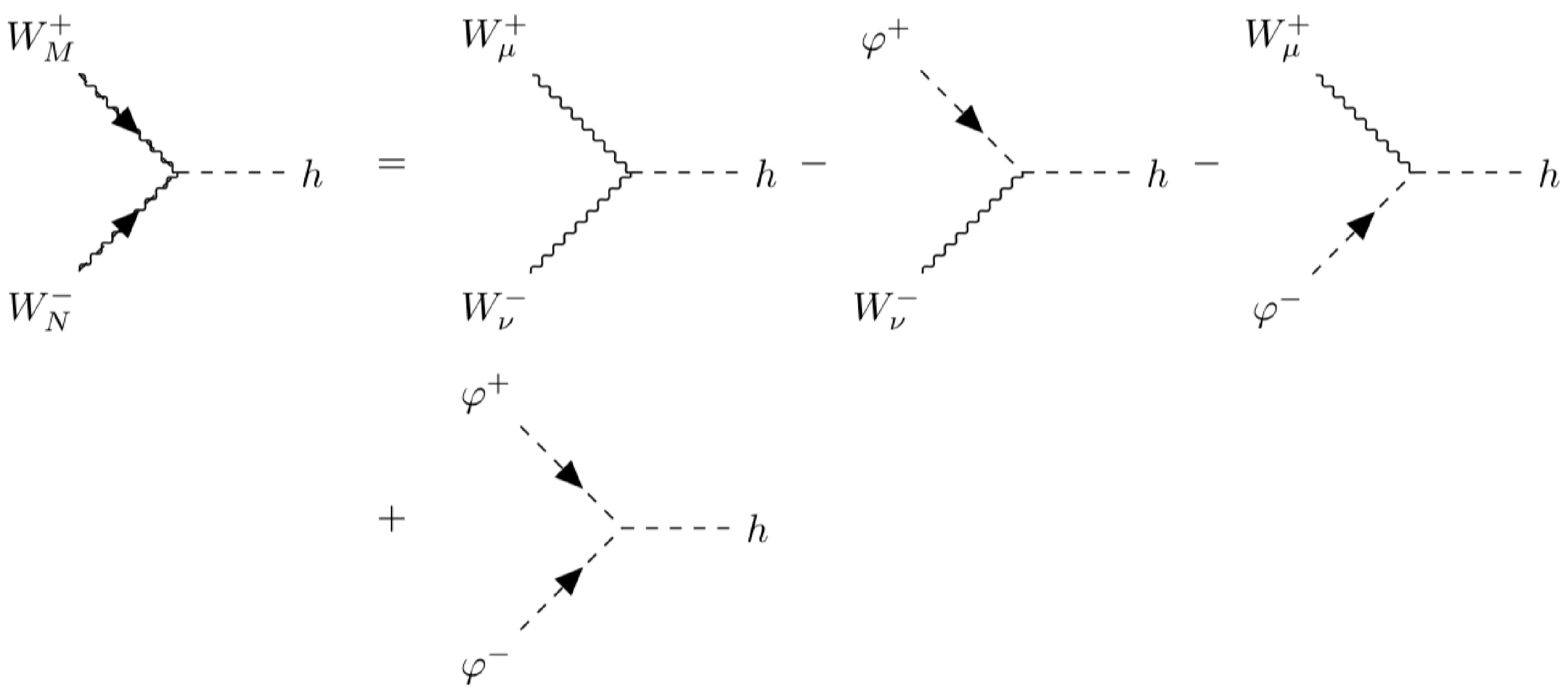
Figure 2.  5-component vertex of $ WWh $ in the double-line notation. The minus sign in front of $ \varphi W h $ comes from the $ g_{44}=-1 $ component of the "metric" $ g_{MN} $.

The new form of vertices brings additional subtleties. As an example, we denote the $ WWh $ vertex to be $ V_{WWh}^{MN} $, where the subscript indicates the vertex and the superscript represents indices. In the GE representation, a vertex involving massive vector bosons has multiple parameters. For instance, $ V^{MN}_{WWh} $ not only includes the pure gauge components $ V^{\mu\nu}_{WWh} $ with coupling $ g_{WWh} $, but also involves the gauge-Goldstone components $ V^{\mu 4}_{WWh} = V^{\mu}_{W\varphi h} $ with coupling $ g_{W\varphi h}=g_{\varphi W h} $ and the pure Goldstone component $ V_{WWh}^{44} = V_{\varphi\varphi h} $ with coupling $ \lambda_{\varphi\varphi h} $. We can further express the vertex as $ V^{MN}_{WWh}(g_{WWh}, g_{\varphi Wh}, \lambda_{\varphi\varphi h}; m_h, m_W) $. These couplings, however, are not independent in the SM. They are all determined by the gauge coupling g, excluding the mass parameters. These relations come from the spontaneous symmetry breaking of the EW theory, reflecting of the underlying gauge symmetry. Similar relations also exist for other vertices such as $ ff'W $, $ WWZ $, etc. Further details will be discussed in Sec. IV.

Finally, let us examine the free parameters in the SM. The EW gauge and Higgs sectors of the SM contain only four free parameters, which we choose to be $ m_W $, g, $ \theta_{\rm{W}} $, and $ m_h $, representing the W boson mass, the $ {\rm{SU}}(2)_{\rm{L}} $ gauge coupling, the weak mixing angle, and the Higgs boson mass, respectively. All other parameters in these sectors are derived from them. For example, the Z boson mass is given by $ m_Z=m_W/\cos\theta_{\rm{W}} $, and the Higgs self-coupling is $ \lambda_h = 2m_h/v^2=g^2 m_h/(2m_W^2) $. In the fermion sector, each Yukawa coupling is defined as $ \lambda_f = g m_f/(\sqrt{2}m_W) $, introducing an additional parameter, the corresponding fermion mass $ m_f $. If we assume that the particle masses have been precisely measured and are treated as inputs, then the free parameters in the EW sectors of the SM reduce to just two: g and $ \theta_{\rm{W}} $.

In this section, we directly test the gauge symmetry in EW scattering amplitudes using the MWI (6). We take the EW processes $ W^+ W^-\rightarrow t \bar t $ and $ W^+W^-\rightarrow W^+W^- $ as two examples, replacing the polarization vectors of W bosons in the amplitudes with the 5-component momenta $ k^{(*)M} $ and computing $ k^M{\cal{M}}_M $ utilizing HELAS in the GE representation.

In Fig. 3, we show $ k^M{\cal{M}}_M $ for $ W^+ W^-\rightarrow t \bar t $ as function of $ \cos\theta $, where θ is the scattering angle in the center-of-mass (CM) system. The CM energy and the azimuthal angle are fixed as $ \sqrt{s} = 1\; {\rm{TeV}} $ and $ \phi = 0 $. In Figs. 3(a) and 3(b), the polarization vector of $ W^+ $ is replaced by $ k^M $, with the helicities of $ t\bar t $ fixed as $ +- $ and the helicity of $ W^- $ set to be $ 0 $ (longitudinal polarization) and $ + $, respectively. In Figs. 3(c) and 3(d), the setup is similar, expect the helicities of $ t\bar t $ are fixed as $ ++ $. The blue solid lines represent the results including all tree-level diagrams, exactly demonstrating the MWI $ k^M{\cal{M}}_M = 0 $. The red dotted and green dashed lines correspond to the results excluding the t-channel diagram and those solely involving the t-channel diagram, respectively. These contributions are precisely opposite to each other, indicating a large and exact cancellation between different diagrams as expected.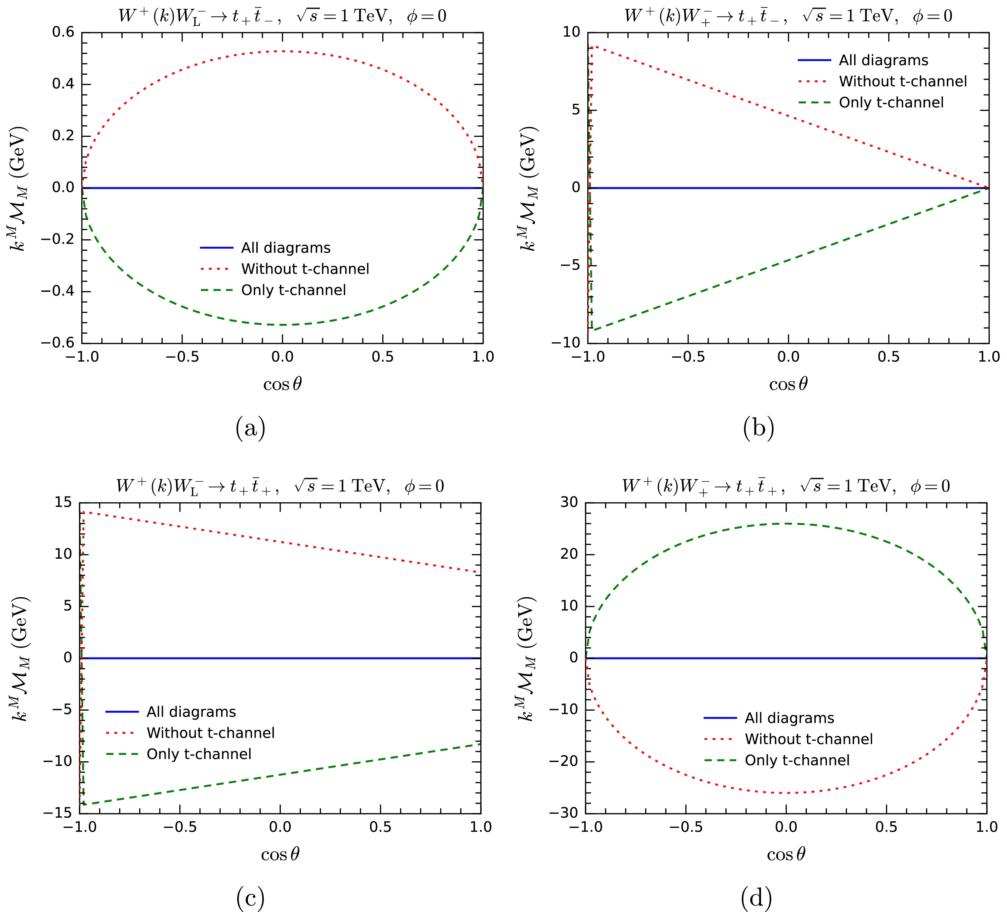

Figure 3.  (color online) Testing the massive Ward identity by computing $ k^M{\cal{M}}_M $ for $ W^+W^-\rightarrow t\bar t $.

In Fig. 4, we present the results for $ W^+W^-\rightarrow W^+W^- $, where one, two, and four polarization vectors of W bosons are replaced by one, two, and four 5-component momenta, respectively. The helicities of the remaining W bosons are uniformly set to $ + $. The blue lines represent the sums of all tree-level diagrams, while the red dotted, green dashed, and black dot-dashed lines correspond to the results for the contact, s-channel, and t-channel diagrams, respectively. Once again, we observe that the MWI is satisfied when all tree-level diagrams are included, confirming the gauge symmetry.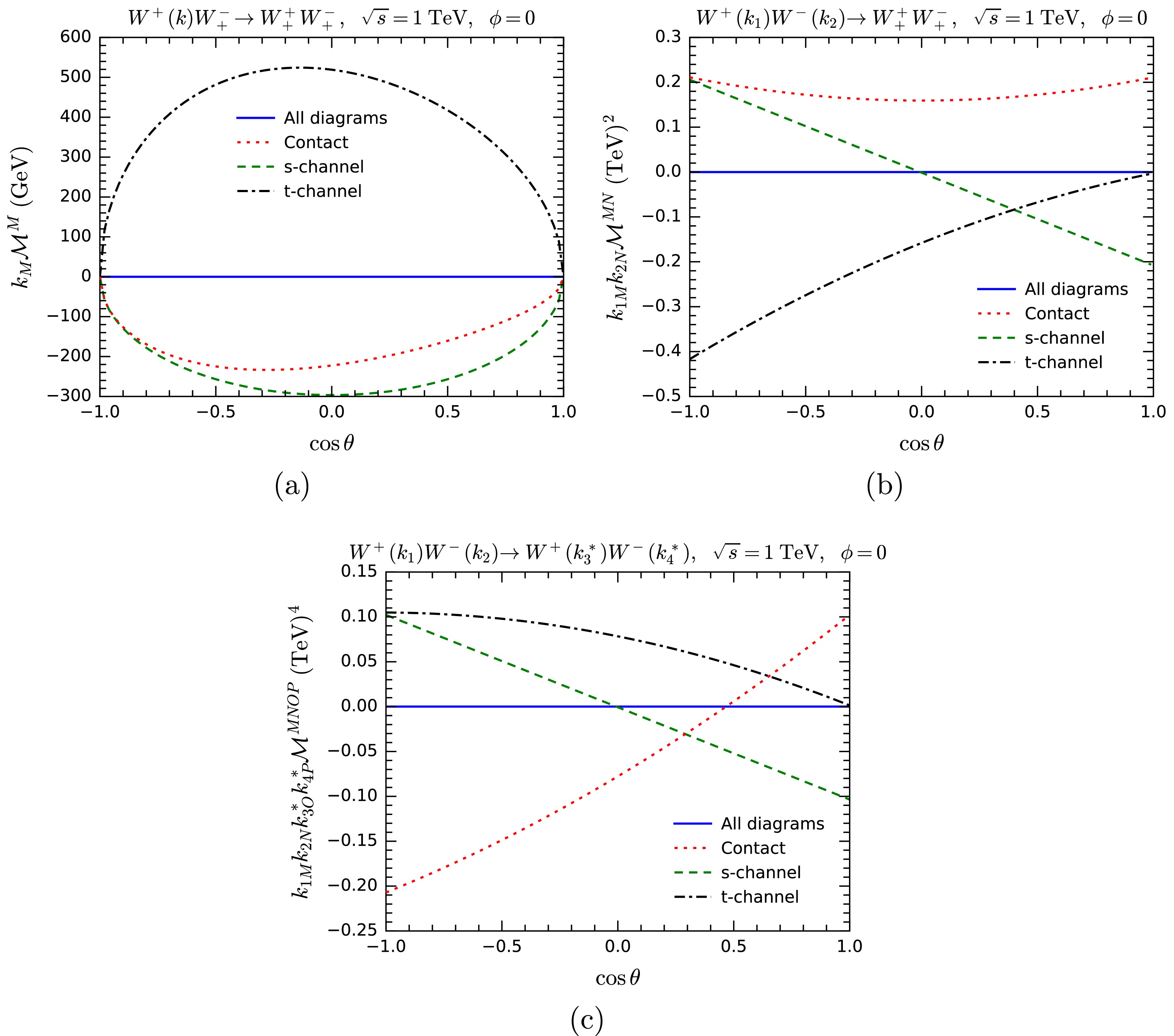

Figure 4.  (color online) Testing the massive Ward identity by computing $ k_M {\cal{M}}^M $ (a), $ k_{1M} k_{2N} {\cal{M}}^{MN} $ (b), and $ k_{1M} k_{2N} k^*_{3O} k^*_{4P} {\cal{M}}^{MNOP} $ for $ W^+W^-\rightarrow W^+W^- $.

In the previous section, we confirmed that the gauge symmetry represented by the MWI ensures precise cancellation among various diagrams when one or multiple polarization vectors $ \epsilon^M(k) $ are replaced by 5-component momenta $ k^M $. In this section, we take a different approach by modifying certain couplings to examine how the MWI is affected. Such a test of gauge symmetry through anomalous couplings can provide deeper insights into how different couplings and parameters are interrelated through gauge symmetry.

In the GE representation, any vertex involving massive vector bosons contains multiple couplings. This allows us not only to modify the couplings of individual vertices as a whole but also to adjust specific parameters within those couplings. The latter will be studied in Subsection IV A with 3-point vertices, while the former will be discussed in Subsection IV B with 4-point vertices.

In this subsection, we examine gauge symmetry through the analysis of 3-point vertices, specifically focusing on the $ VVh $, $ ff'V $, and $ VVV $ vertices within the GE representation.

$ VVh $ vertex

The first type of vertices we study is the $ VVh $ vertices, which include the $ WWh $ and $ ZZh $ vertices. As discussed in Sec. II, a $ VVh $ vertex in the GE representation involves four sub-vertices: $ VVh $, $ V\varphi h $, $ V\varphi h $, and $ \varphi\varphi h $, with corresponding couplings $ g_{hVV} $, $ g_{V\varphi h} $, $ g_{\varphi V h} $, and $ \lambda_{\varphi\varphi h} $. For the $ WWh $ vertex in the SM, the couplings are related to each other by the following relations:

We intend to test the MWI by modifying these couplings by

The SM corresponds to $ \delta^1_{WWh}=\delta^2_{WWh}=\delta^3_{WWh}= \delta^4_{WWh}=0 $. For the $ ZZh $ vertex, we only need to replace $ m_W $ with $ m_Z $ in Eqs. (12) and (13). To facilitate a clearer comparison with the gauge representation, we leave $ g_{WWh} $ unchanged, ensuring $ \delta_{WWh}^1=0 $ at all times. Additionally, we enforce $ \delta^2_{WWh}=\delta^3_{WWh}\equiv \delta^{23}_{WWh} $ when modifying the couplings, as the two sub-vertices $ V\varphi h $ and $ \varphi V h $ belong to the same type.

The processes we choose to test gauge symmetry with the $ WWh $ vertex are $ W^+ W^-\rightarrow t\bar t $ and $ W^+ W^-\rightarrow hh $. We first compare the cross sections vs. $ \delta_{WWh}^{23,4} $ in both the unitary gauge and the GE representation, the results are shown in Fig. 5. Just as expected, when $ \delta^{23}_{WWh} $ and $ \delta^4_{WWh} $ are nonzero, the cross sections in the GE representation deviate from those in the unitary gauge, which remain unchanged and retain the SM values. The larger $ \delta^{23}_{WWh} $ and $ \delta^4_{WWh} $ are, the larger are the deviations. Compared to $ WW\rightarrow hh $, $ WW\rightarrow t \bar t $ exhibits significantly lower sensitivity to $ \delta^{23}_{WWh} $ and $ \delta^4_{WWh} $. We have to plot $ \delta^{23}_{WWh} $ and $ \delta^4_{WWh} $ over the range $ [-100,100] $ for $ WW\rightarrow t \bar t $, but only $ [-1, 1] $ for $ WW\rightarrow hh $. It is not surprising, given that the $ WWh $ vertex contributes to three channels of $ WW\rightarrow hh $, but only one in $ WW\rightarrow t\bar t $. Another notable observation is that the sensitivity of cross section is much higher to $ \delta^{23}_{WWh} $ than $ \delta^4_{WWh} $ for $ WW\rightarrow h h $, but the sensitivities are approximately the same for $ WW\rightarrow t\bar t $.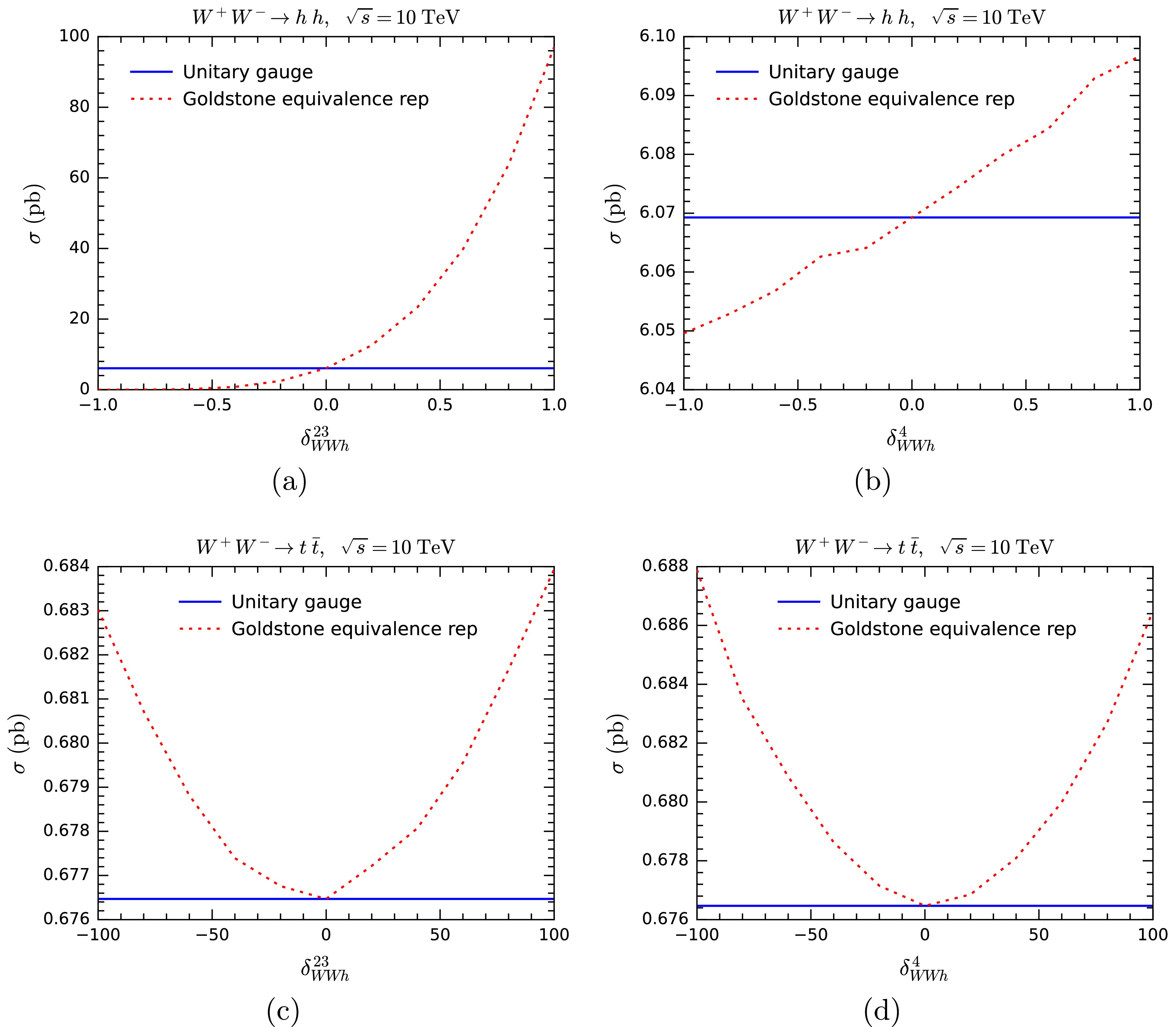

Figure 5.  (color online) Cross sections of $ WW\rightarrow hh $ (upper panels) and $ WW\rightarrow t \bar t $ (lower panels) at $ \sqrt{s} = 10\; {\rm{TeV}} $ with varying $ \delta^{23}_{WWh} $ and $ \delta^4_{WWh} $ in the unitary gauge (blue solid lines) and the GE representation (red dotted lines).

Next, we compute $ k_M{\cal{M}}^M $ or $ k_{1M} k_{2N} {\cal{M}}^{MN} $ for these processes as a way of testing gauge symmetry by replacing polarization vectors of one or two W bosons with 5-component momenta. The results are shown in Fig. 6 for $ WW\rightarrow hh $ and Fig. 7 for $ WW\rightarrow t\bar t $, respectively. For $ WW\rightarrow t\bar t $, we analyze various helicity combinations. In certain helicity configurations, the results consistently vanish due to the violation of angular momentum conservation. Apart from these cases, the anomalous couplings lead to violations of the MWI. For $ WW\rightarrow t\bar t $, the deviations for $ \delta^{23}_{WWh} $ are larger than those for $ \delta^4_{WWh} $.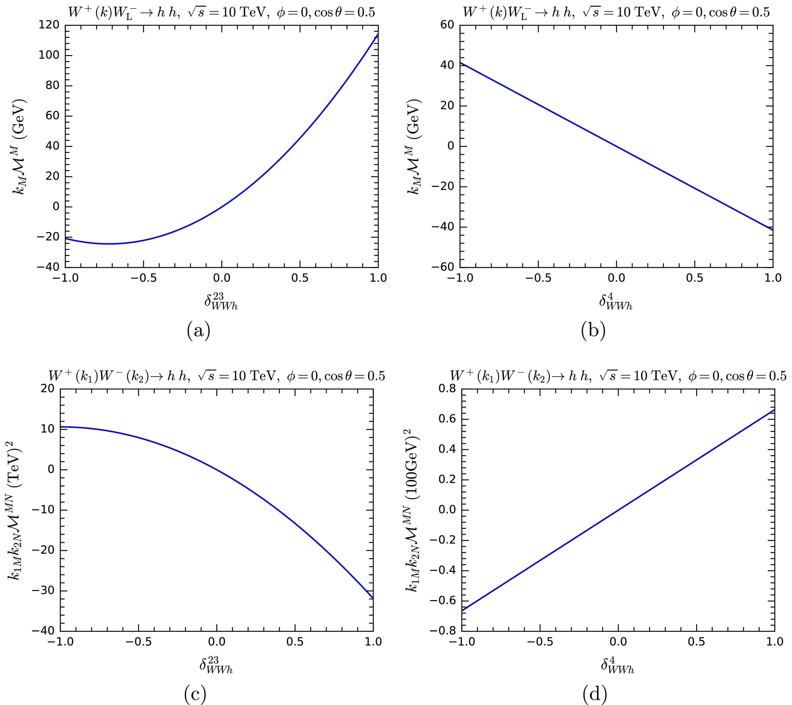

Figure 6.  (color online) $ k_M{\cal{M}}^M $ and $ k_{1M} k_{2N} {\cal{M}}^{MN} $ as functions of $ \delta^{23}_{WWh} $ and $ \delta^4_{WWh} $ for $ WW\rightarrow hh $ with one or two W polarization vectors are replaced by 5-component momenta.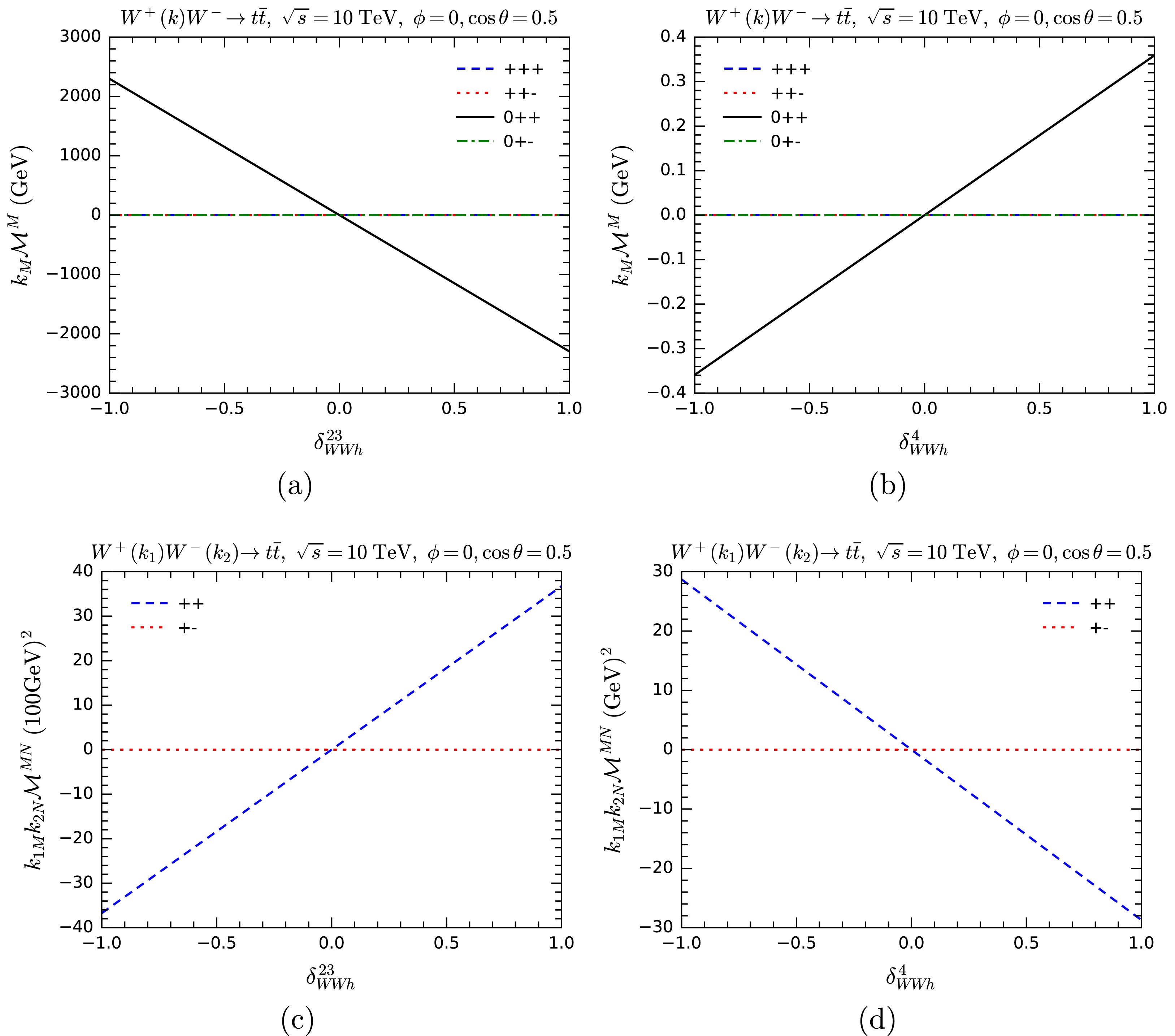

Figure 7.  (color online) $ k_M{\cal{M}}^M $ and $ k_{1M} k_{2N} {\cal{M}}^{MN} $ as functions of $ \delta^{23}_{WWh} $ and $ \delta^4_{WWh} $ for $ WW\rightarrow t\bar t $ with one or two W polarization vectors are replaced by 5-component momenta. Results for various helicity combinations are shown.

$ ff'V $ vertex

The $ ff'V $ vertex has two sub-vertices: $ ff'V $ and $ ff'\varphi $. The $ ff'V $ coupling can be parameterized as $ -i \gamma^\mu (g_{\rm{L}} P_{\rm{L}} + g_{\rm{R}} P_{\rm{R}}) $, while the $ ff'\varphi $ coupling is $ y_{\rm{L}} P_{\rm{L}} + y_{\rm{R}} P_{\rm{R}} $. Just like the $ VVh $ case, gauge couplings and Yukawa couplings are not independent, as the latter can be expressed in terms of the former.

For a charged current vertex such as $ u\bar d W $, we have

For a neutral current vertex such as $ u\bar u Z $, we have

with $ s_{\rm{W}} \equiv \sin \theta_{\rm{W}} $ and $ c_{\rm{W}} \equiv \cos \theta_{\rm{W}} $. To sum up, the $ ff'\varphi $ couplings are essentially Yukawa couplings $ y_f $, which are related to the fermion masses $ m_f $ by $ y_f = g m_f/(\sqrt{2}m_W) $. This relation is protected by gauge symmetry, and therefore the breaking of gauge symmetry will be reflected on violation of this relation.

Similar to $ VVh $, we test gauge symmetry by modifying the $ ff'V $ couplings as following:

The process we choose to examine gauge symmetry for the $ ff'V $ vertex is $ WW\rightarrow t\bar t $. This process is ideal because its t-channel diagram includes the $ t\bar b W $ vertex, while its s-channel diagram includes the $ t\bar t Z $ vertex, allowing us to examine both charged and neutral currents.

In Fig. 8, we demonstrate how the $ WW\rightarrow t\bar{t} $ cross sections are changed when the couplings $ y_{ttZ}^{{\rm{L}}/{\rm{R}}} $ and $ y_{tbW}^{b/t} $ are modified in both the unitary gauge and the GE representation. Similarly, we show how $ k_M{\cal{M}}^M $ or $ k_{1M} k_{2N}{\cal{M}}^{MN} $ change with the anomalous $ tbW $ couplings in Fig. 9, and with the anomalous $ ttZ $ coupling in Fig. 10, respectively. As the figures show, gauge symmetry is broken when one of the components of $ tbW/ttZ $ couplings are modified, both in terms of cross sections and the MWI. For $ ttZ $, the sensitivity of $ k_M{\cal{M}}^M $ and $ k_{1M} k_{2N}{\cal{M}}^{MN} $ to $ \delta_{ttZ}^{\rm{L}} $ is much higher than $ \delta_{ttZ}^{\rm{R}} $. This is expected, since the SM $ ttZ $ vertex is dominated by the left-handed interaction. For $ tbW $, the sensitivity to $ \delta_{tbW}^t $ is much higher than $ \delta_{tbW}^b $. The reason is also not hard to see: the top Yukawa coupling is much larger than the bottom Yukawa coupling.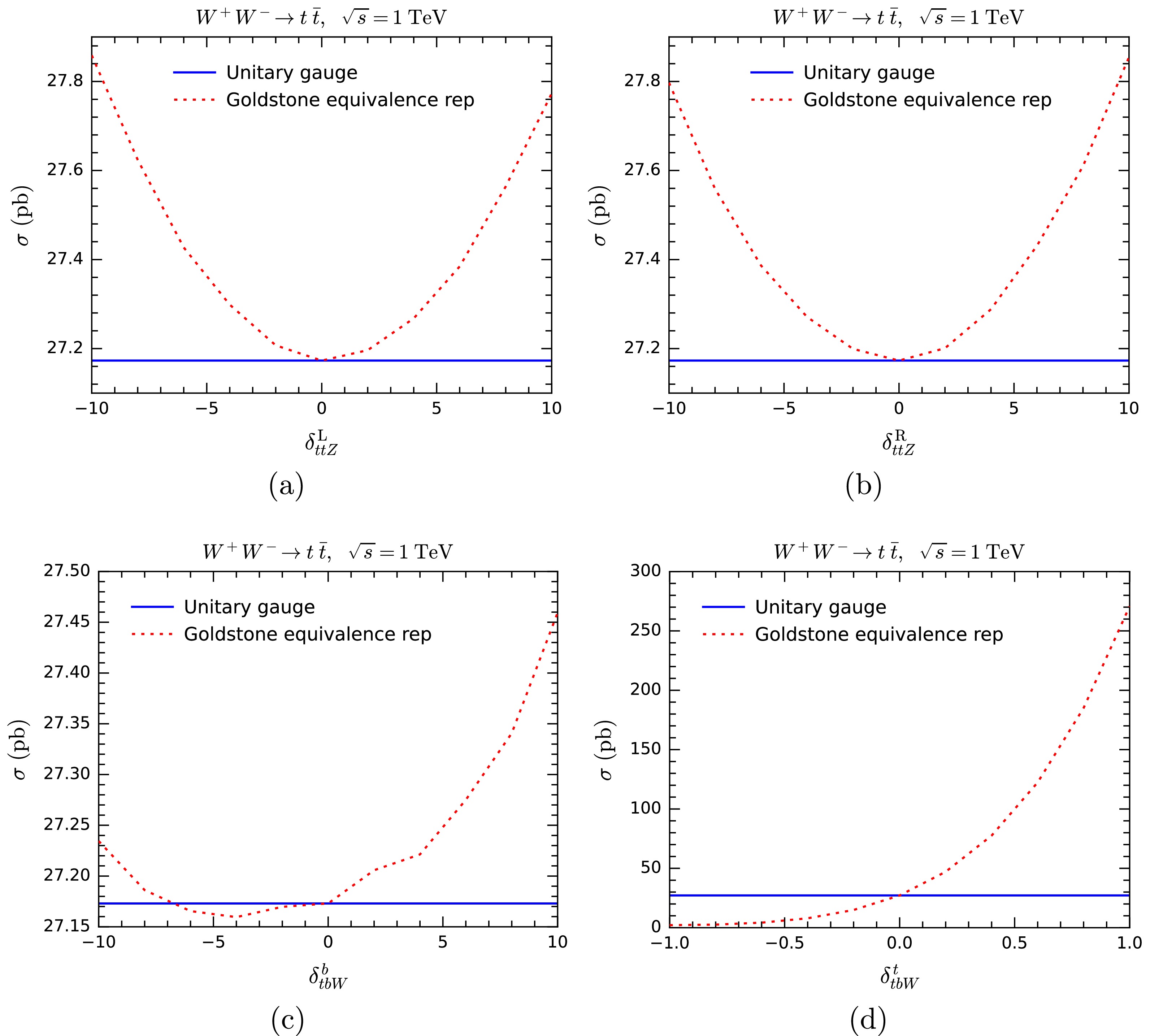

Figure 8.  (color online) Cross sections of $ WW\rightarrow t\bar{t} $ in the unitary gauge and the GE representation as functions of anomalous couplings of $ ttZ $ (upper panels) and $ tbW $ (lower panels).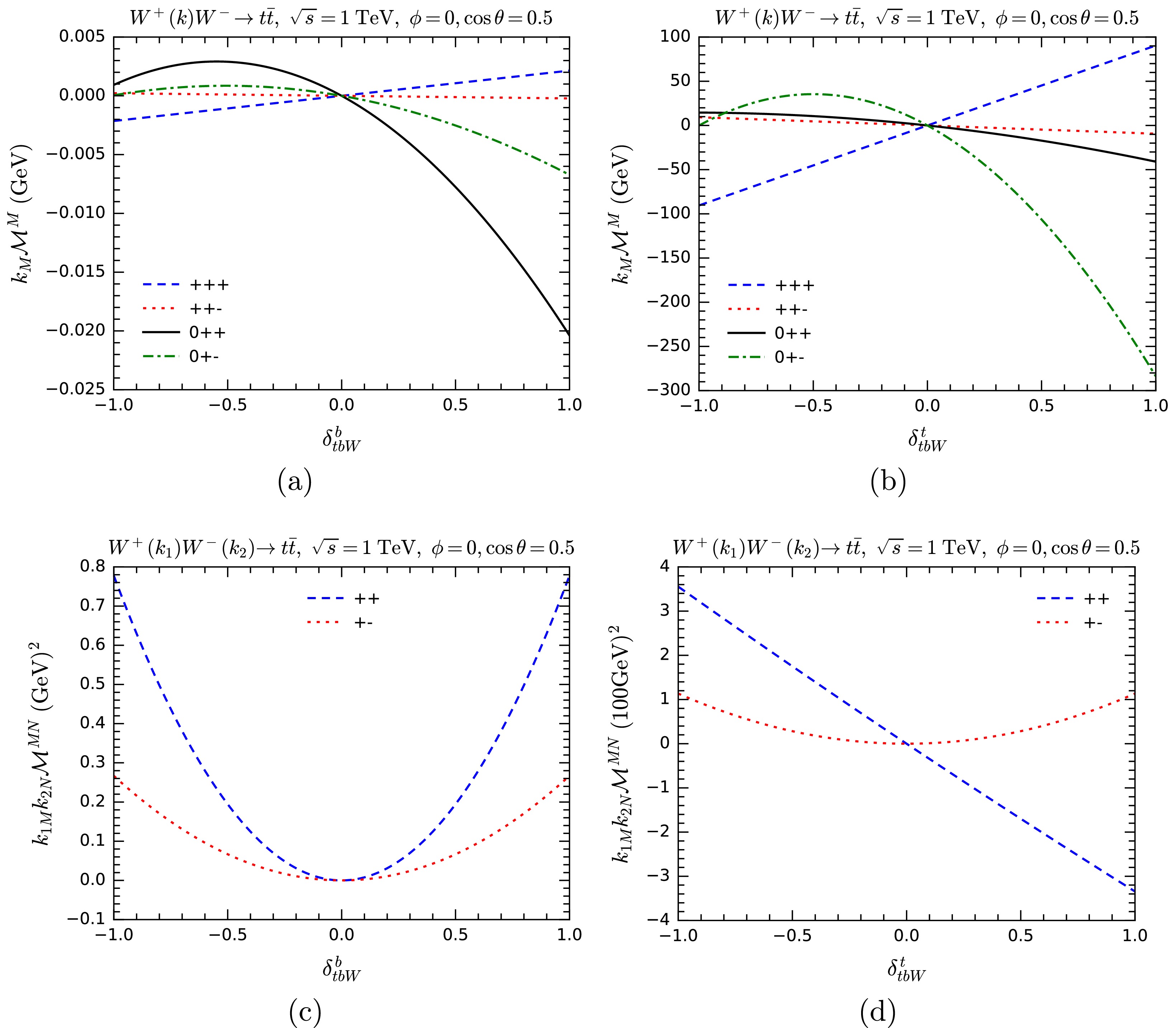

Figure 9.  (color online) Testing the MWI by computing $ k_M{\cal{M}}^M $ (upper panels) and $ k_{1M} k_{2N}{\cal{M}}^{MN} $ (lower panels) with anomalous $ tbW $ couplings for the process $ WW\rightarrow t\bar t $. Various helicity combinations are shown.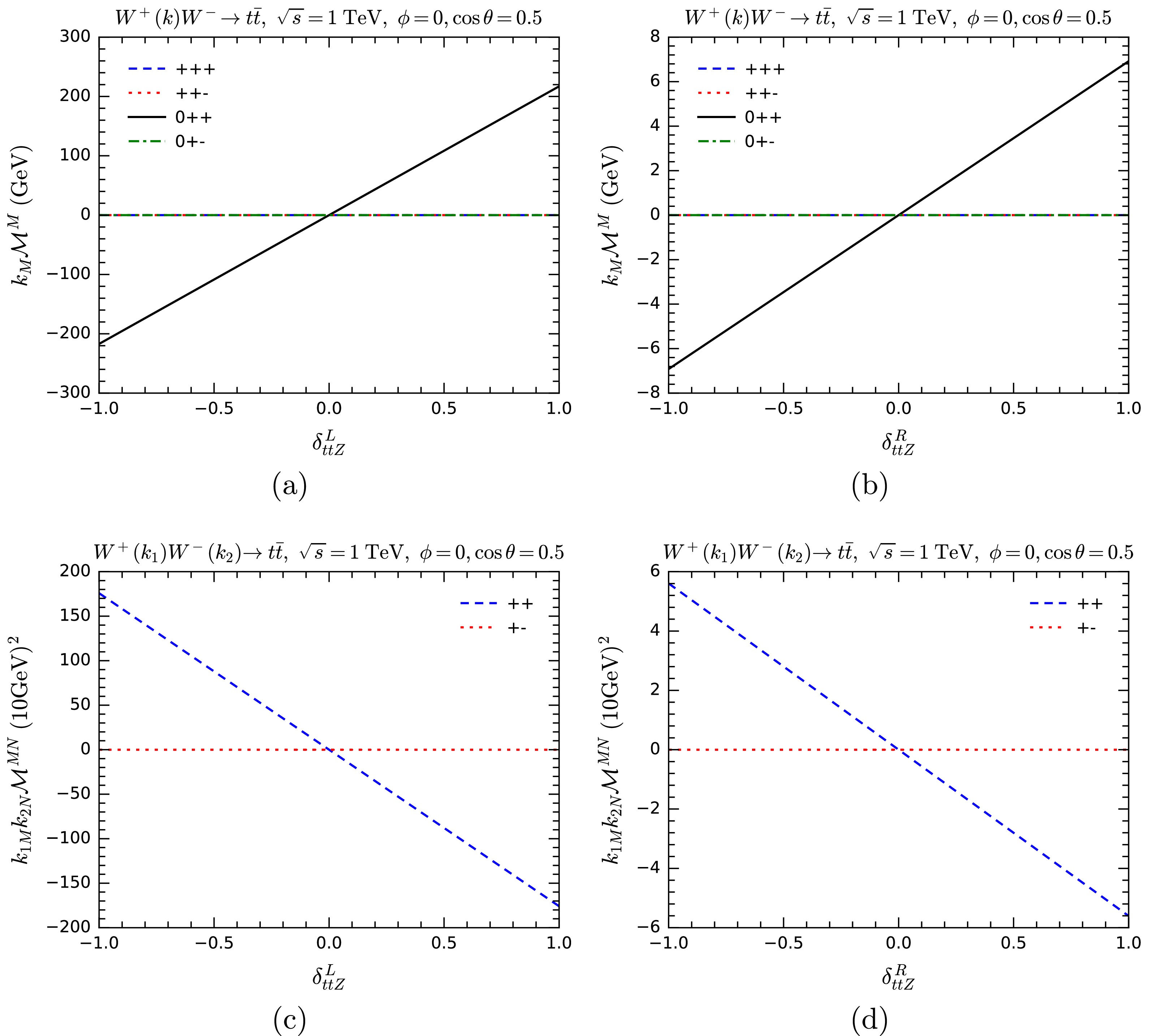

Figure 10.  (color online) Testing the MWI by computing $ k_M{\cal{M}}^M $ (upper panels) and $ k_{1M} k_{2N}{\cal{M}}^{MN} $ (lower panels) with anomalous $ ttZ $ couplings for the process $ WW\rightarrow t\bar t $. Various helicity combinations are shown.

$ VVV $ vertex

In the SM, there two $ VVV $ vertices, $ W^+W^+Z $ and $ W^+W^-A $, either of which has 3 types of sub-vertices: $ VVV $, $ V\varphi V $, and $ \varphi\varphi V $. There is no $ \varphi\varphi\varphi $-type vertex.

For the $ WWZ $ vertex, the couplings are related to each other by

with $ c_{2{\rm{W}}}\equiv \cos 2\theta_{\rm{W}} $ and $ e = g s_{\rm{W}} $. Following the analysis for the $ VVh $ and $ ff'V $ vertices, we modify the couplings to test gauge symmetry as following:

We examine gauge symmetry of the $ WWZ $ vertex with both the $ W^+ W^+ \rightarrow W^+ W^- $ and $ WW\rightarrow t\bar t $ processes. In Figs. 11 and 12, we test the MWI by modifying $ \delta_{WWZ}^{234} $ and $ \delta_{WWZ}^{567} $ for $ W^+ W^+ \rightarrow W^+ W^- $ and $ WW\rightarrow t\bar t $, respectively. In both cases, the sensitivity of the violation of the MWI to $ \delta_{WWZ}^{567} $ is higher than $ \delta_{WWZ}^{234} $, sometimes significantly so. This is somewhat surprising, since the $ VV\varphi $-type vertex that $ \delta_{WWZ}^{567} $ modifies is suppressed by $ e = g s_{\rm{W}} $. However, they are typically proportional to $ m_W $, providing an enhancement that effectively counterbalances the suppressive influence of the weak mixing angle $ \theta_{\rm{W}} $.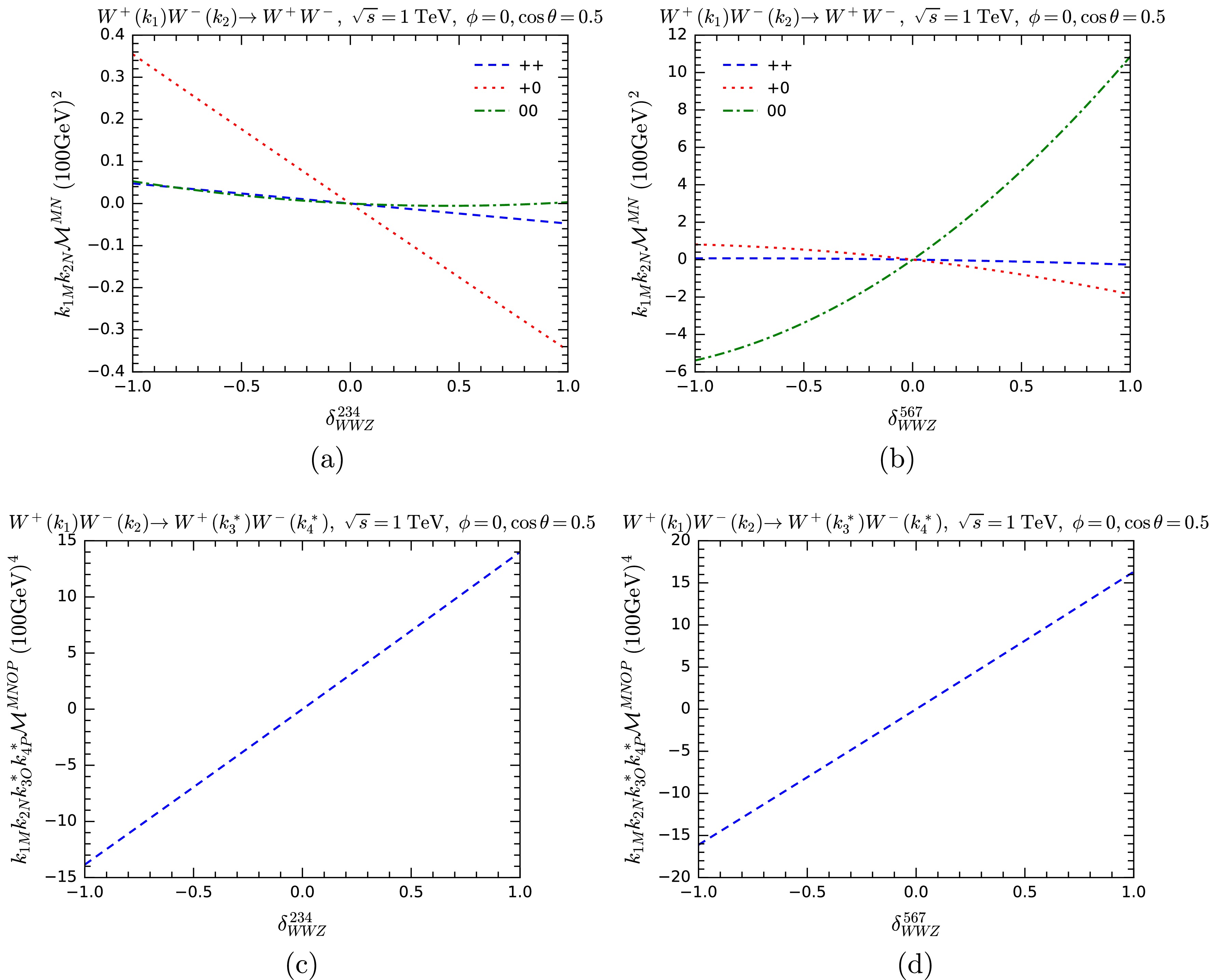

Figure 11.  (color online) Testing the MWI by computing $ k_{1M} k_{2N} {\cal{M}}^{MN} $ (upper panels), and $ k_{1M} k_{2N} k^*_{3O} k^*_{4P} {\cal{M}}^{MNOP} $ (lower panels) with anomalous $ WWZ $ couplings for the process $ W^+ W^+ \rightarrow W^+ W^- $. In the upper panels, various helicity combinations are shown.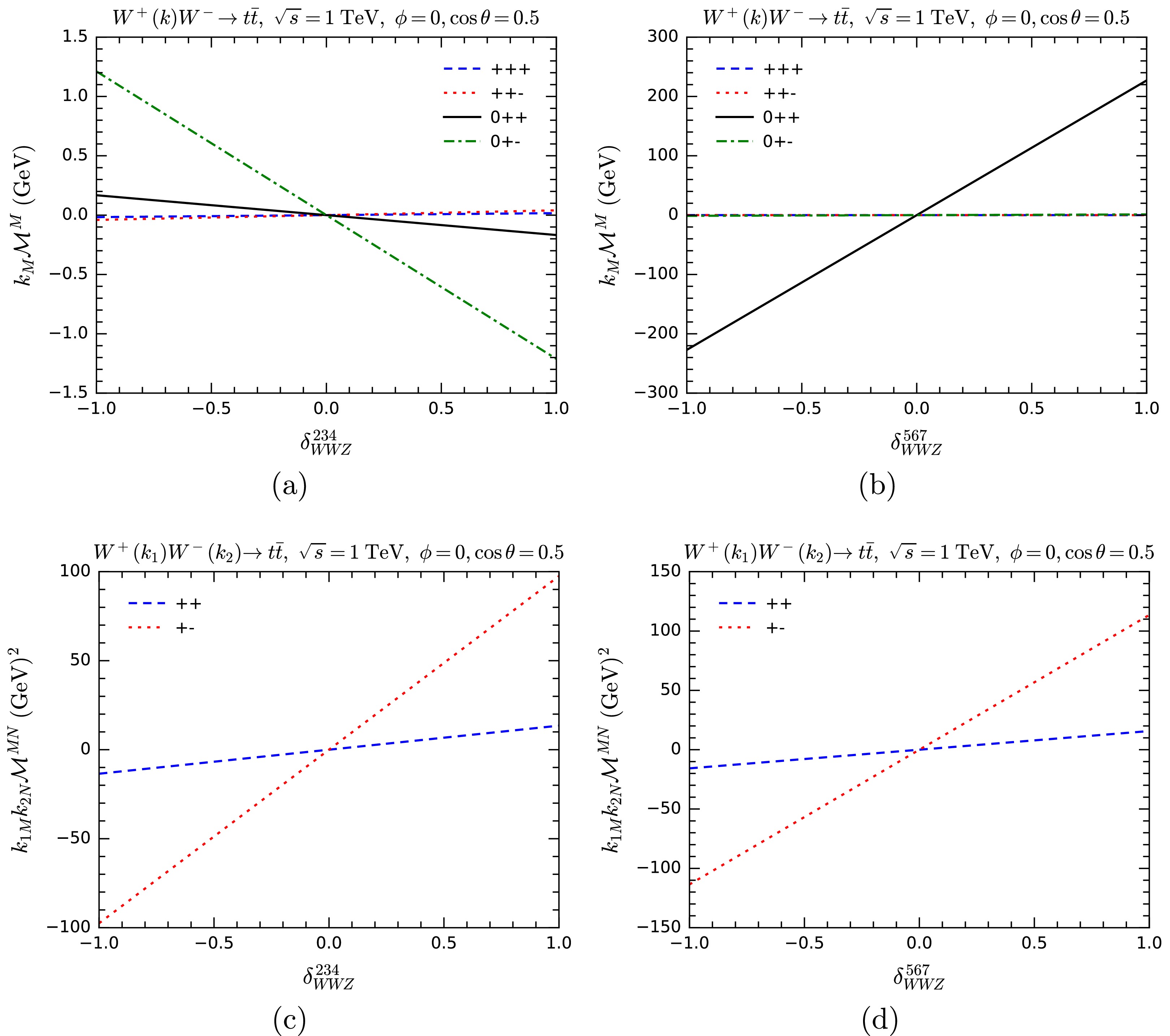

Figure 12.  (color online) Testing the MWI by computing $ k_M{\cal{M}}^M $ (upper panels) and $ k_{1M} k_{2N} {\cal{M}}^{MN} $ (lower panels) with anomalous $ WWZ $ couplings for the the process $ WW\rightarrow t\bar t $. Various helicity combinations are shown.

Gauge symmetry is not only reflected in the couplings within a single vertex, but also in the relations among different vertices. For example, in the $ WW\rightarrow W W $ process, where vertices such as $ WWWW $, $ WWZ $, $ WW\gamma $, and $ WWh $ are involved, the MWI requires precise relations among their couplings. Any deviation from the SM values breaks gauge symmetry, similar to how it violate unitarity in the gauge representation. We will modify the overall couplings of the vertices to test the MWI. The processes we choose are $ W^+ W^-\rightarrow W^+ W^- $, $ W^+ W^-\rightarrow hh $, and $ W^+ W^-\rightarrow t\bar t $.

For $ W^+ W^-\rightarrow W^+ W^- $, we separately vary the overall couplings of the $ WWh $, $ WWZ $, and $ WWWW $ vertices and compute $ k_M {\cal{M}}^M $. In Fig. 13, we show the results, listing different helicity combinations in the process. As expected, we can see the violation of the MWI when the anomalous couplings are nonzero. This violation is most sensitive to $ \delta_{WWZ} $ and $ \delta_{WWWW} $.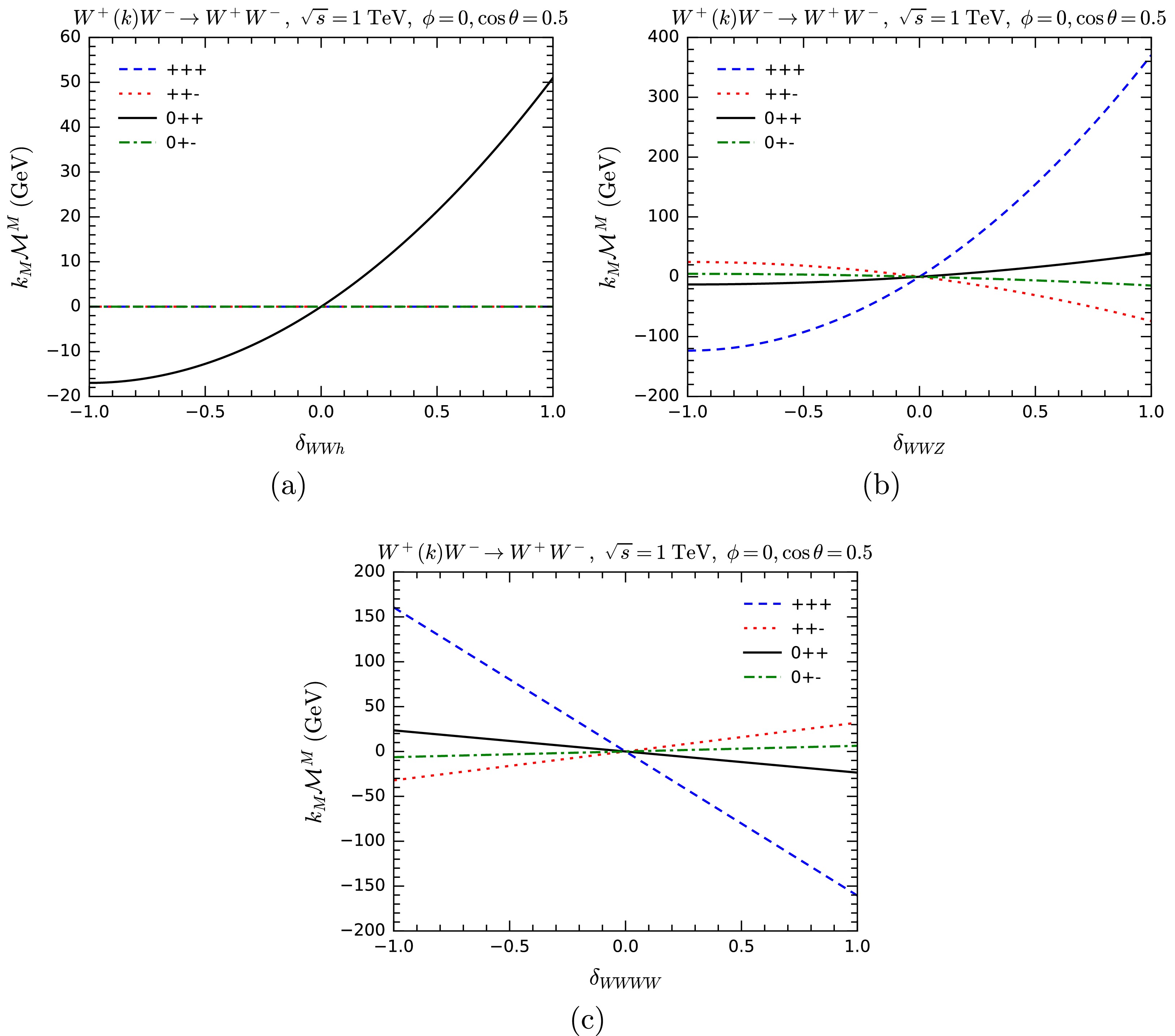

Figure 13.  (color online) $ k_M{\cal{M}}^M $ for $ W^+ W^-\rightarrow W^+ W^- $ as functions of anomalous overall couplings $ \delta_{WWh} $ (a), $ \delta_{WWZ} $ (b), and $ \delta_{WWWW} $ (c). Various helicity combinations are shown.

One interesting observation is that, in most helicity combinations, $ k_M {\cal{M}}^M $ remains zero or close to zero. This reminds us to be careful in selecting helicities when testing gauge symmetry of massive amplitudes. The exact vanishing of $ k_M {\cal{M}}^M $ in the presence of an anomalous $ \delta_{WWh} $ appears to be due to angular momentum conservation: the amplitude vanishes when angular momentum conservation is violated, so only helicity combinations that conserve angular momentum can yield nonzero values.

For $ WW\rightarrow hh $, we separately modify the couplings of the $ hhh $, $ WWh $, and $ WWhh $ vertices, and compute $ k_M{\cal{M}}^M $. The results are shown in Fig. 14.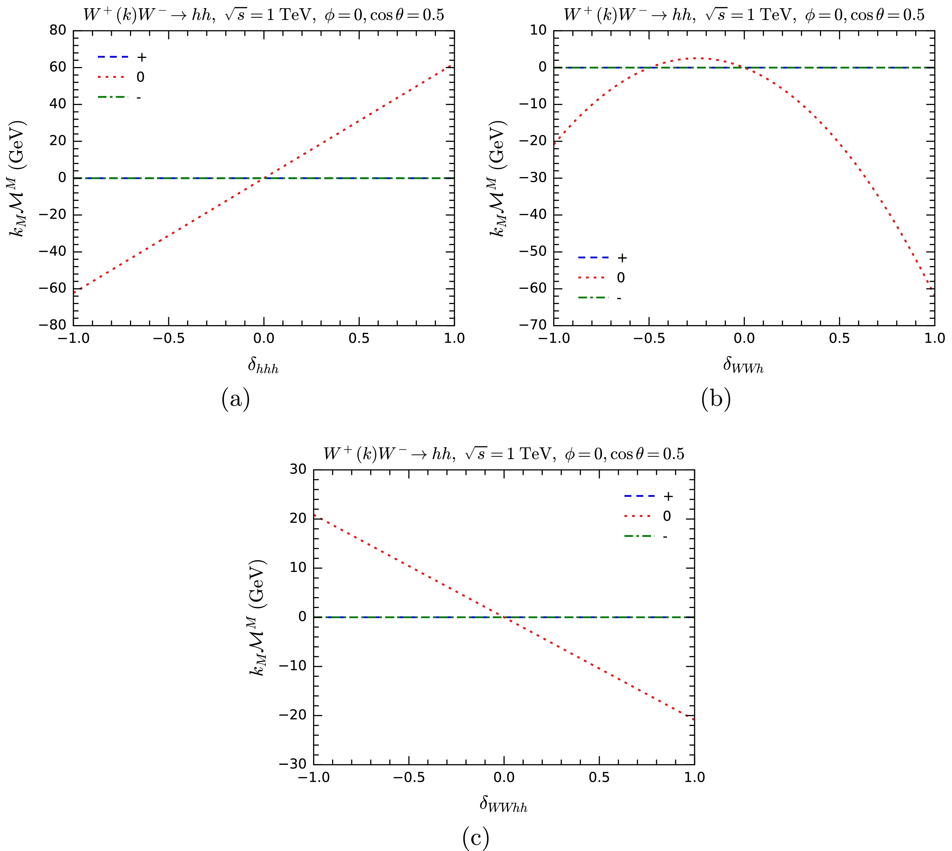

Figure 14.  (color online) $ k_M{\cal{M}}^M $ for $ WW\rightarrow hh $ as functions of anomalous overall couplings $ \delta_{hhh} $ (a), $ \delta_{WWh} $ (b), and $ \delta_{WWhh} $ (c). Various helicity configurations are shown.

For $ WW\rightarrow t\bar t $, we separately modify the couplings of the $ tbW $, $ ttZ $, and $ tth $ vertices. The results are shown in Fig. 15.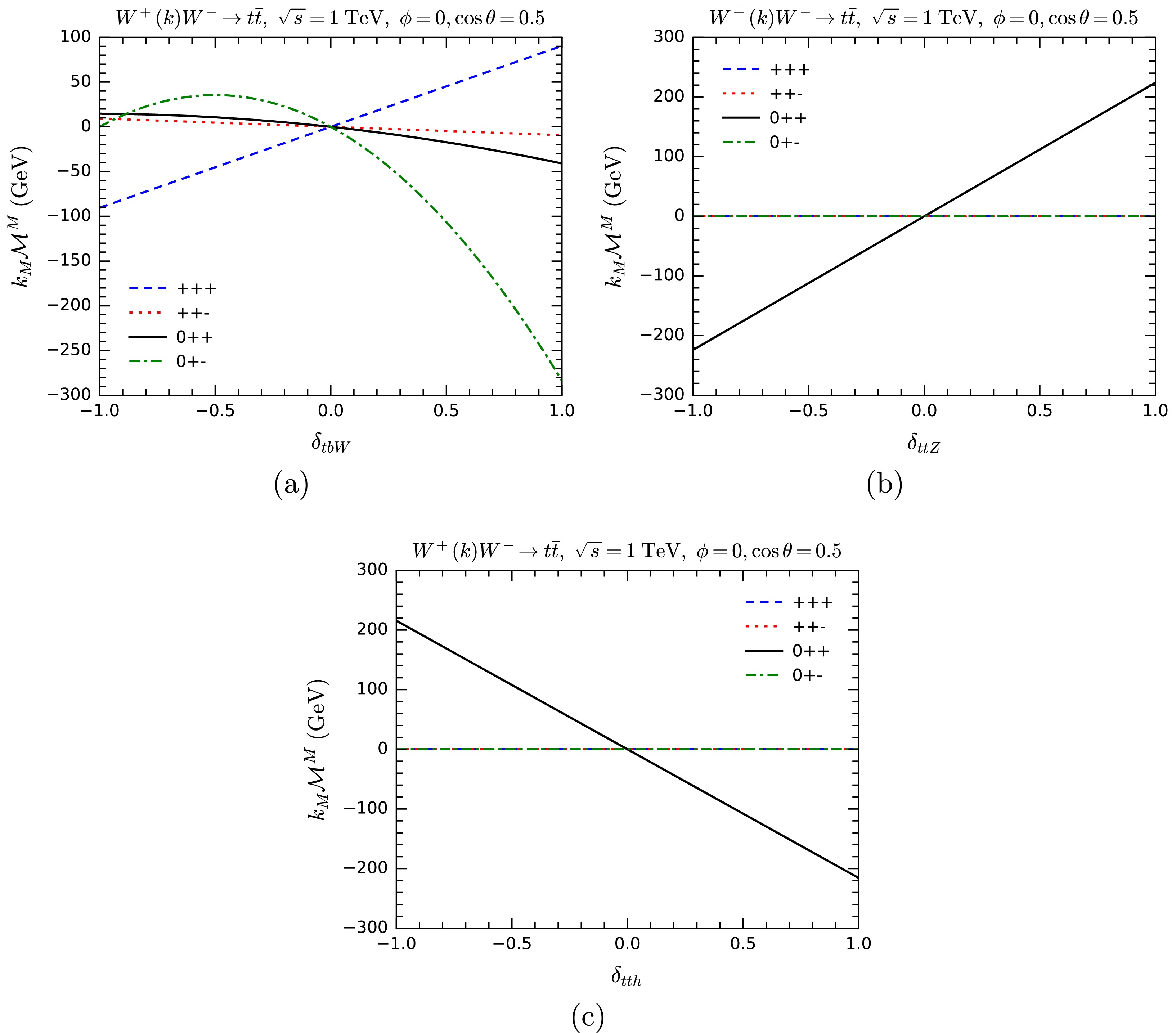

Figure 15.  (color online) $ k_M{\cal{M}}^M $ for $ WW\rightarrow t\bar t $ as functions of anomalous overall couplings $ \delta_{tbW} $ (a), $ \delta_{ttZ} $ (b), and $ \delta_{tth} $ (c). Various helicity combinations are shown.

The overall pattern is similar for all three processes. Angular conservation forbids some helicity combinations, giving $ k_M{\cal{M}}^M = 0 $ automatically, no matter how the couplings of individual vertices are modified. This, however, does not mean that the MWI is valid regardless of the couplings. Because there are always some helicity combinations, in which a modification of one coupling results in the violation of the MWI.

So far the anomalous couplings we considered are only instruments to demonstrate the gauge symmetry of related amplitudes. They do not have intrinsic, gauge-invariant, physical meanings. However, there is a scenario that anomalous couplings can be physical. That is when those couplings are part of a set of anomalous SM couplings from new physics that respects gauge symmetry. An example that we will explore in this section is SMEFT, which is an effective field theory respecting the SM gauge symmetry. In particular, we will discuss two dim-6 SMEFT operators [27−30]: $ {\cal{O}}_6=C_6(\Phi^\dagger \Phi)^3 $ and $ {\cal{O}}_{t\Phi}=C_{t\Phi}(\Phi^\dagger \Phi)(\bar Q_{\rm{L}} t_{\rm{R}}\tilde \Phi) + {\rm{H.c.}} $, where Φ is the SM Higgs doublet and $ \tilde\Phi \equiv i\sigma^2 \Phi^* $. We will study how the gauge symmetry is restored in the presence of these operators when the 3-point Higgs self-coupling $ \lambda_{hhh} $ and the top Yukawa coupling $ y_{tth} $ are modified in the $ WW\rightarrow h h $ and $ WW\rightarrow t\bar t $ processes, respectively.

$ WW\rightarrow h h $

Adding an SMEFT operator $ {\cal{O}}_6=C_6(\Phi^\dagger \Phi)^3 $ into the SM Lagrangian, the $ hhh $ and $ hh\varphi^+\varphi^- $ couplings are modified to

Since the two couplings are modified by the same operator, their deviations from the SM values are related. This relation is further protected by gauge symmetry. Conversely, if we modify one of the couplings alone, say $ \lambda_{hhh}=\lambda_{hhh}^{\rm{SM}}+\delta_{hhh} $, the gauge symmetry will be broken. In order to restore gauge symmetry, the other coupling $ \lambda_{hh\varphi^+\varphi^-} $ has to be modified by adding

Any deviation from the above relation will break gauge symmetry for a process involving both $ hhh $ and $ hhVV $ couplings, which can be tested with the MWI.

In order to test the relation (20), we introduce a deviation parameter δ by

Thus, $ \delta = 0 $ corresponds to the relation (20) that respects gauge symmetry. We take $ \delta_{hhh} $ to be $ 0.2 $, $ 0.4 $, $ 0.8 $, and $ 1 $. For every $ \delta_{hhh} $ value, we compute $ k_M{\cal{M}}^M $ as a function of δ for the $ WW\rightarrow h h $ process with one W polarization vector replaced by the 5-component momentum. The results are summarized in Fig. 16. As can be seen in the figure, $ k_M{\cal{M}}^M = 0 $ only appears when $ \delta =0 $, i.e., when the relation (20) holds. This confirms our argument that, with an anomalous coupling of $ \lambda_{hhh} $, gauge symmetry can be restored by adding an proper anomalous coupling of $ \lambda_{hh\varphi\varphi} $.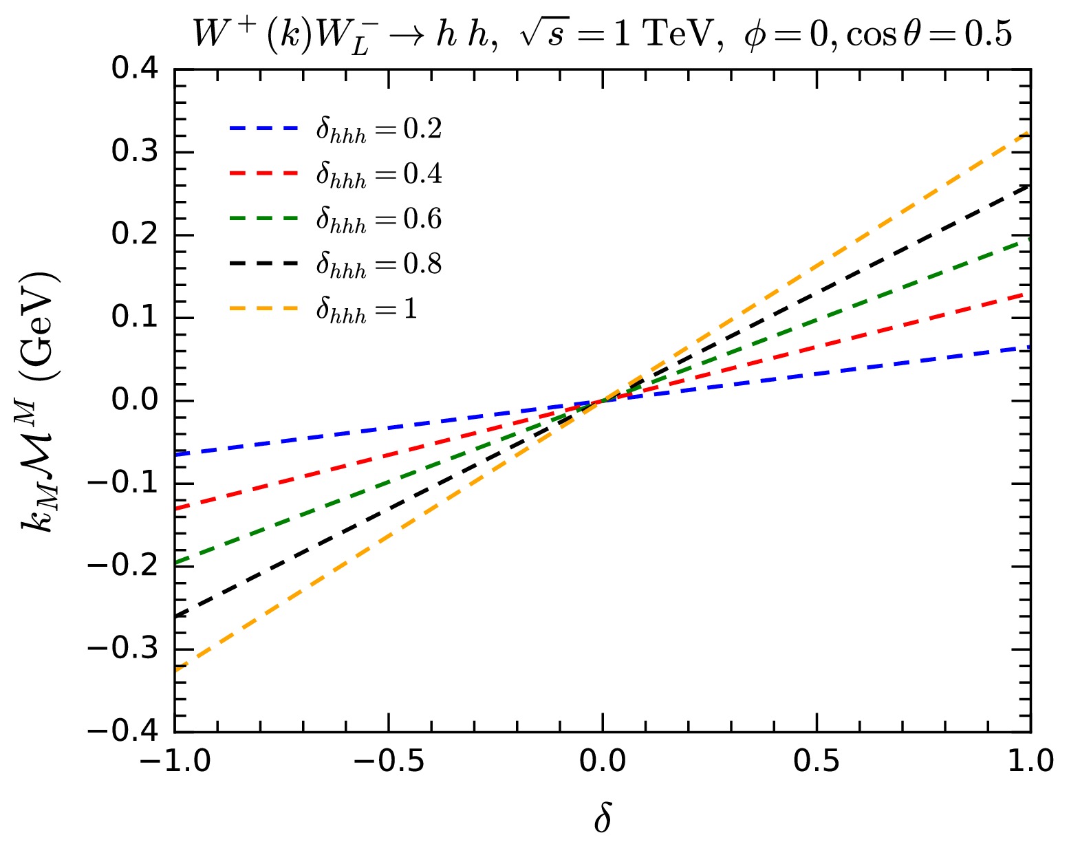

Figure 16.  (color online) $ k_M{\cal{M}}^M $ for $ WW\rightarrow hh $ as functions of δ with different values of $ \delta_{hhh} $, serving as a test for gauge symmetry in the presence of the SMEFT operator $ {\cal{O}}_6 $.

$ WW\rightarrow t\bar t $

We then focus on gauge symmetry of the $ WW\rightarrow t\bar t $ process with the incorporation of the SMEFT operator $ {\cal{O}}_{t\Phi}=C_{t\Phi}(\Phi^\dagger \Phi)(\bar Q_{\rm{L}} t_{\rm{R}}\tilde \Phi) + {\rm{H.c.}} $. The couplings of $ tth $ and $ tt\varphi\varphi $ are defined as

In the SM, the values of these couplings are

After the addition of $ {\cal{O}}_{t\varPhi} $, the couplings are modified into

Following the above equations, we can obtain the relations between the modifications to these couplings are

If expressing in left-handed and right-handed couplings, the Lagrangian terms for the $ \bar tth $ and $ tt\varphi\varphi $ couplings become

The modifications to $ y_{\rm{L}} $, $ y_{\rm{R}} $, $ g_{\rm{L}} $, and $ g_{\rm{R}} $ are related to $ C_{t\Phi} $ as

It is easy to see that they are related to each other by

Our method of testing the gauge symmetry is similar to $ WW\rightarrow hh $ with the $ {\cal{O}}_6 $ operator. Two deviation parameters $ \delta_{\rm{L}} $ and $ \delta_{\rm{R}} $ are introduced by

Therefore, $ \delta_{\rm{L}} = \delta_{\rm{R}} = 0 $ corresponds to the modifications contributed by the $ {\cal{O}}_{t\Phi} $ operator that preserve gauge symmetry. In Figs. 17(a) and 17(b), we show $ k_M{\cal{M}}^M $ for $ WW\rightarrow t\bar{t} $ as functions of $ \delta_{\rm{L}} $ and $ \delta_{\rm{R}} $ assuming various values of $ \operatorname{Re}(\delta_{tth}) $ and $ \operatorname{Im}(\delta_{tth}) $, where $ \delta_{tth} $ is defined as $ \delta_{tth} \equiv C_{t\Phi} v^2/\sqrt{2} $. As expected, gauge symmetry is restored when the condition (30) is satisfied. This demonstrates that an anomalous Yukawa coupling can be counterbalanced by a corresponding $ ff\varphi\varphi $ contact vertex, ensuring that the $ WW\rightarrow t\bar{t} $ amplitude remains gauge invariant.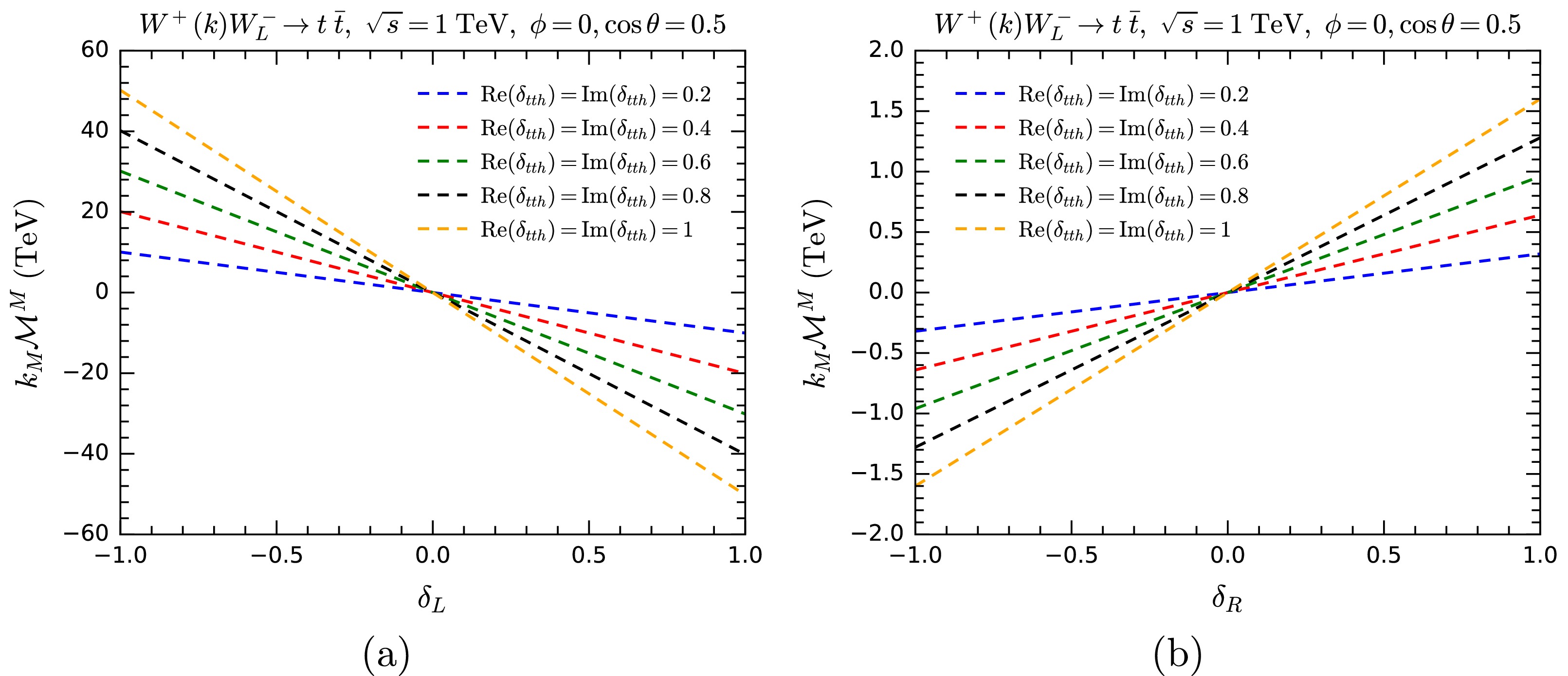

Figure 17.  (color online) $ k_M{\cal{M}}^M $ for $ WW\rightarrow t\bar{t} $ as functions of $ \delta_{\rm{L}} $ (a) and $ \delta_{\rm{R}} $ (b) with different values of $ \operatorname{Re}(\delta_{tth}) $ and $ \operatorname{Im}(\delta_{tth}) $, serving as a test for gauge symmetry in the presence of the SMEFT operator $ {\cal{O}}_{t\Phi} $.

In this paper, we demonstrated that the GE representation of EW interactions, which we had an brief introduction first, has gauge symmetry imprinted in the structure of amplitudes, manifesting in the MWI (1). This approach to gauge symmetry is rarely studied before, because it involves vertices of both gauge bosons and Goldstone bosons simultaneously. We numerically studied this important property of EW interactions in the GE representation in many different aspects, including directly testing the MWI, modifying couplings within vertices, and modifying overall couplings of vertices. Generally, we found that there are precise relations both within and without overall vertices, which guarantee the MWI. Any violation of these relations results in the violation of the MWI and gauge symmetry.

By directly testing gauge symmetry on 4-point amplitudes such as $ WW\rightarrow t\bar t $ and $ W^+ W^- \rightarrow W^+ W^- $ with different helicity combinations, we found that the full amplitudes always satisfy the MWI after summing over all tree-level diagrams. This result typically involves large cancellations between individual diagrams, similar to unitarity cancellation in the gauge representation.

For testing gauge symmetry on 3-point vertices with anomalous couplings, we studied the $ VVh $, $ ff'V $, and $ VVV $ vertices. We found that there are precise relations governing the couplings of Goldstone and gauge components for these vertices. We then numerically test if the MWI still holds when some of the couplings are modified so that those relations are violated. What we found is that any deviation from those relations by anomalous couplings would violate the MWI.

For testing gauge symmetry on 4-point amplitudes with anomalous couplings, we studied $ W^+ W^+\rightarrow W^+ W^+ $, $ WW\rightarrow hh $, and $ WW\rightarrow t\bar t $. We focused on how modifying the overall couplings of individual vertices affects gauge symmetry. Our results are similar to 3-point vertices: gauge symmetry is manifested as precise relations between couplings, and modifying couplings to violate those relations also results in violating the MWI.

After studying gauge symmetry of the SM, we then proceed to study effective operators in the SMEFT, specifically the $ {\cal{O}}_6 $ operator that modifies the Higgs self-couplings and the $ {\cal{O}}_{t\Phi} $ operator that modifies the top Yukawa coupling. We found that the operators modify both the couplings mentioned and the related Goldstone couplings, giving relations between the couplings involving $ C_6 $ and $ C_{t\Phi} $, respectively. Numerically testing the MWI indicates that gauge symmetry is preserved as long as all related couplings are modified in accordance with those relations. On the other hand, if those relations are violated, gauge symmetry would be broken. Similar to the SM, our results for these SMEFT operators demonstrate that not only the gauge components but also the Goldstone components are crucial for maintaining gauge invariance of the theory. This is also the reason why gauge cancellation in the unitary gauge, in which there is no Goldstone mode, seems ad hoc without obvious physical mechanism.

We believe that this paper contributes to a deeper understanding of EW interactions and massive gauge theory in general. In addition, it also gives a convenient way of checking self-consistency of EW interactions in the GE representation.

So far the 5-component formalism has been only systematically implemented in HELAS for the tree-level Feynman rules of the SM. Besides, for the purpose of this work, we also included the dim-6 operators $ {\cal{O}}_6 $ and $ {\cal{O}}_{t\Phi} $ in HELAS. However, the majority of the SMEFT operators remain to be incorporated. This obviously limits the utility of our method and calls for more progress in this aspect. In Ref. [12], a general method for automatically implementing the 5-component framework was proposed recently, giving hope to apply our method to more general theories.

The authors thank Kaoru Hagiwara for helpful discussions.