Comparison of the description of yrast bands in the Harris and IBM models for even nuclei Th and U

Visualization of the behavior of the energies of states E in a band becomes more qualitative if we move from energies to effective moments of inertia J. This also allows us to improve the method of comparing experimental and calculated energies of states of one band.

In addition, the backbending effect can be used to form judgments about the spin values at which the bands cross. Comparison of the $ J(\omega^2) $ curves obtained from experimental energies with those given by various nuclear models, including microscopic ones, can reveal the capabilities of the corresponding models and provide more reasoned judgments about the nature and character of the states.

One of the methods of reproducing and predicting energies is based on the expansion of the moment of inertia in powers of the rotation frequency ω, as in the Harris model [1]. This is justified when the transition to a new band has not yet occurred in the rotation band. As a rule, such a transition occurs quite quickly in one or two states of the yrast band. In this case, this is shown on the graph of the moment of inertia versus the square of the rotation frequency in a specific way through backbending. Among heavy nuclei, starting with thorium isotopes, three such nuclei are known today: ²²⁰Th, ²⁴²Pu, and ²⁴⁴Pu. This is why in [2], within the framework of the IBM1 [3] phenomenology (hereinafter referred to as IBM), a good description of the energies of yrast bands up to extremely high spins I in heavy nuclei from Pu to No was obtained. The effective moment of inertia and the square of the rotational frequency are defined as

This paper presents a description of the energies of yrast bands in even-even heavy nuclei in the Harris model, considered not from the point of view of the cracking model, but as a phenomenological model with a number of parameters no more than four. The possibility of IBM in its phenomenological aspect to describe moments of inertia is also considered. IBM phenomenology is understood as a description of the energies of collective states in nuclei through fitting the parameters both of the boson Hamiltonian and the maximum number of quadrupole bosons. The moments of inertia obtained in the two models are compared with each other. Finally, the task is set to develop a criterion for determining the spin at which the crossing of bands occurs. This can be done based on a comparison of the behavior of $ J(\omega^2) $ according to experimental data and what the Harris model gives. It should be noted that in some cases, although backbending may not be observed, the crossing of bands is still possible. This was revealed by microscopic description of the chain of isotopes ^220-236Th [4]. The microscopic version of IBM developed by us is presented in [4] and in the references therein. In it, based on the effective factorized forces, the boson parameters are calculated. In addition, due to the expansion of the boson space by bosons with multipolarity up to to $ J=14^+ $, it becomes possible to describe the phenomenon of band crossing in nuclei. Calculations within the Harris scheme are made for all the presented nuclei. For ^220,222Th the results are presented also within the IBM microscopic framework. For for ²²⁶Th and U isotopes the IBM phenomenology also was used in calculations.

In order to increase the calculated moment of inertia at high-spin states in deformed nuclei (^162,164Er), in [5], a new term was incorporated into the Hamiltonian of IBM, so that $ I(I+1)\rightarrow I(I+1)/(1+fI(I+1)) $. This part of the Hamiltonian is always diagonal for any values of the parameters $ H_{\rm{IBM}} $. This addition is motivated by the fact that a decrease in superfluidity, the gap parameter, leads to an increase in the moment of inertia, and the gap parameter decreases with increasing rotation frequency. This should lead to $ dJ/dI>0 $ and $ dJ/d \omega >0 $. Here, however, it should be kept in mind that the growth of the moment of inertia from the rotation frequency is achieved with arbitrary values of the traditional and full Hamiltonian of IBM, except for the one that corresponds to the case of the $ SU(3) $ limit of IBM. In addition, with the growth of the spin of the collective state, the influence of two-quasiparticle states on the energy of this state increases. One example of a band built on a two-quasiparticle mode is the S band. This also leads to an additional increase in the moment of inertia or a decrease in the energies of intra-band transitions.

Analysis of the dynamic moments of inertia of the lowest superdeformed (SD) bands in even-even Hg, Pb, Gd, and Dy [6] and ^192,194Hg, ^152,154Dy [7] isotopes led to the need to extend the coefficient f so that considering only the relative excitation of the states in a rotational band, the energy of the state with angular momentum I can be simply expressed as

Introduction of an additional modification of the Arima coefficient f shows that J can change nonmonotonously with rotational frequency. Up to the point that as the spin increases, the positive slope of the moment of inertia from the rotation frequency can change to negative. The latter, by analogy with the terms ``backbending'' and ``upbending'', can be called downbending.

Calculations on this basis belong to semi-phenomenological approaches.

In [8], a novel modification is introduced, extending the Arima coefficient to the third order. The computed outcomes of the rotational bands of ²⁴⁴Pu and ²⁴⁸Cm demonstrate an exceptional degree of agreement with experimental observations. Moreover, the used parameterization of the Arima term and its modification successfully describes such behavior of the moment of inertia from frequency as backbending, upbending, and the downturn (down bending).

Commenting on the considered series of works [5–8], it should be kept in mind that the phenomenon of backbending is traditionally associated with the intersection of bands of different nature, namely, the collective one, built on the ground state, and the one that has a two-quasiparticle pair with a sufficiently high spin at its base.

The upbending phenomenon may be due to the fact that the crossing of bands has not yet occurred completely, but the situation is close to it. In addition, the growth of the slope of the moment of inertia from frequency within certain limits is reproduced within the framework of the traditional, but at the same time complete IBM Hamiltonian.

From a microscopic point of view, as the spin of states increases, the average number of quadrupole bosons increases, and this leads to some weakening of pairing. Accordingly, the introduction of the Arima modification of the IBM Hamiltonian was motivated by this decrease in pairing correlation due to the increase in rotation. At the same time, this leads to an increase in the energy of the quasiparticle vacuum or a decrease in the correspon ding depth.

In this case, with an increase in the spin of the collective state, a decrease in the microscopically calculated energy of the d boson $ \varepsilon_d $ occurs (the corresponding term also arises when using only the $ \hat{Q}\cdot \hat{Q} $ interaction by reducing the last operator to the normal order over bosons). Since IBM assumes that the energy of the boson vacuum is constant, a redistribution of the variable part of the energy of the quasiparticle vacuum is made over two boson parameters $ \varepsilon_d $ and $ k_1 $ (see below (8)). This results in the d-boson energy practically ceasing to change, and the energy of the boson vacuum remaining unchanged. This procedure is described in [9–11] and clearly demonstra- ted in [11].

Thus, the weakening of pairing during the unwinding of the nucleus by the values of the parameters of the boson Hamiltonian is significantly leveled out.

There is one more effect left, this is the weakening of the growth of the moment of inertia with frequency at high spins − downturn or downbending. It can be assumed that the IBM specificity, namely, the finiteness of the maximum number of quadrupole bosons, can reproduce this phenomenon [12] without introducing the Arima modifications to the boson Hamiltonian. Introducing the Arima modification is convenient if we remain in the $ SU(3) $ approximation of the IBM limit. In this case, this modification approximates a more complex dynamics of collective motions in the nucleus, described in the general case by the $ SU(6) $ group.

In [13], the structure of yrast bands in the transuranium nuclei ²⁴²Pu and ²⁴⁴Pu was investigated within the framework of the projected shell model. This approach is completely microscopic.

The description of rotational bands at ultra-high spins within the framework of covariant density functional theory for the $ A\geq 242 $ actinides was presented in [14].

The rotational bands properties of plutonium isotopes ^236-246Pu were studied [15] via projected shell model. The results of the calculated energy levels of the yrast band were compared with experimental data and a good agreement has been found. The crossing between two-quasiparticle (2qp) excited bands and the ground state band (g-band) in the high-spin regions has been analyzed in terms of band diagrams. The upbendings are observed in the kinematic moments of inertia curves for ^236-246Pu isotopes.

The objectives of this work are defined as:

1) obtaining a precise description of the energies of yrast bands in even-even heavy nuclei in the Harris model;

2) comparison of the behavior of $ J(\omega^2) $ in the Harris and IBM models both in its phenomenological aspect and in the aspect of its extension by taking into account high-spin modes;

3) development of a criterion for determining the spin at which the crossing of bands occurs without resorting to microscopic calculations;

4) identification of the causes, conditions and values of the spins of collective states when the downturn or downbending effect occurs.

We will use the Harris model [1] in its phenomenological aspect. If we assume that the following decomposition is valid

then the effective moment of inertia will have the form

With fixed values of parameters $ J_0, J_1, J_2, J_3 $, the rotation frequencies are found from the equation

For each value of the spin of state I, the value $ \omega=\omega_I $ is found. The energies of the states of the main band are found as

where $ E_0=0. $ The parameters that determine the moment of inertia (3) are found by minimizing the value

or standard deviation

where $ I_{\rm{fit}} $ is the maximum spin of the states and the bands by which the parameters $ J_0, J_1, J_2, J_3 $ are determined.

The results obtained in the Harris model will be related to the results in the IBM phenomenology. The parameterization of its Hamiltonian is taken as

$ \rm{H.c.} $ means Hermitian conjugation, the dot between the operators corresponds to the scalar product, the quantities $ \varepsilon_d, k_1, k_2, C_0, C_2, C_4 $ are the parameters of the model. The total number of bosons or the maximum number of d bosons will be denoted as Ω. For several nuclei, results will be presented within the framework of the extended microscopic version of IBM, where high-spin excitation modes are also considered, without disclosing its content here, but only making a reference to the work [4].

The next section discusses the energies of the yrast band states of even thorium isotopes in comparison with the results of the Harris model phenomenology, and for several nuclei with IBM.

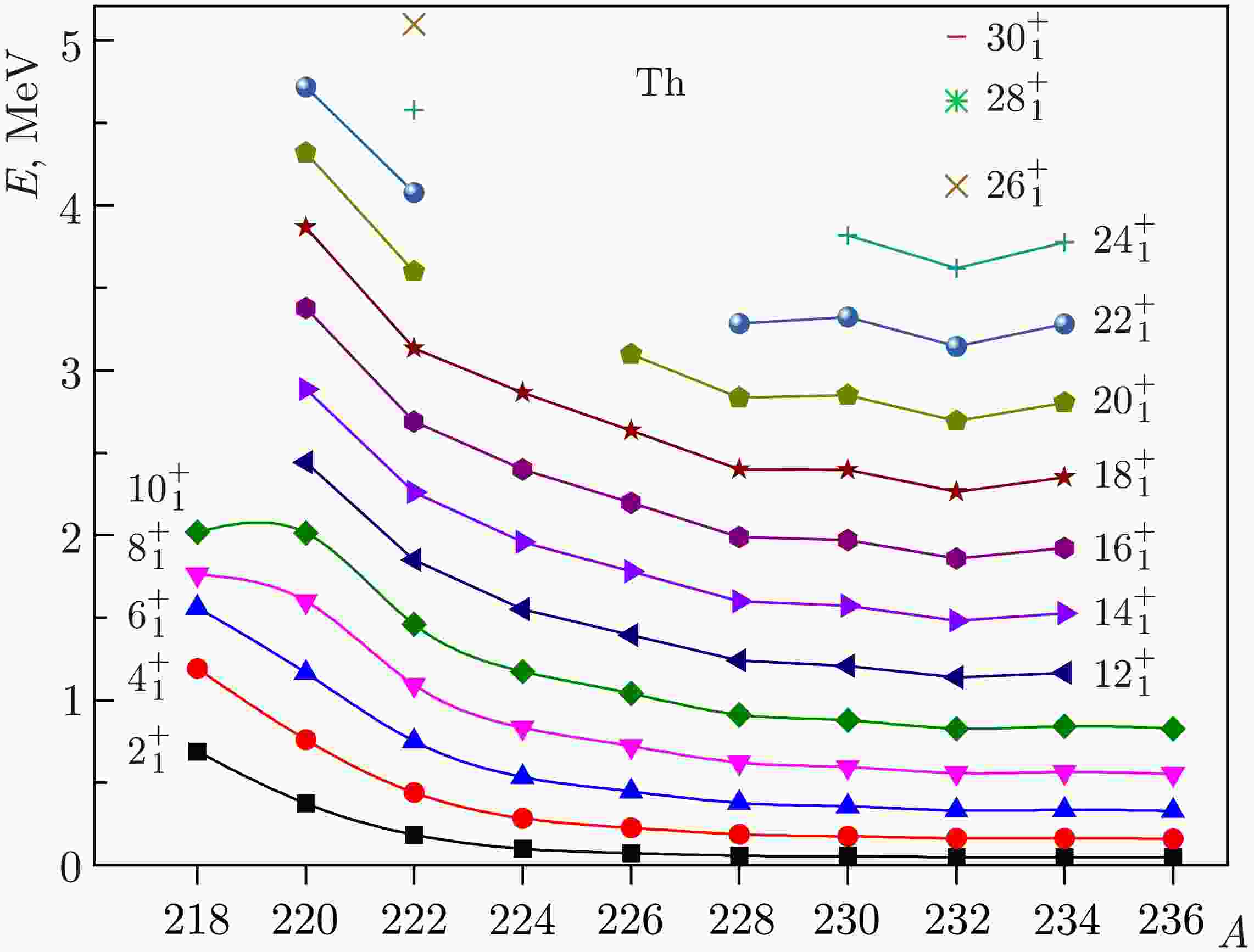
Figure 1 presents a visual systematics of the energies of the corresponding states. It is evident that the energies of states with spins $ I\leq 10^+ $ decrease at first to $ A=224 $ rather quickly, and at large nucleon values, the energies decrease quite smoothly, so that $ E(2^+_1)=48.4 $ keV for ²³⁶Th. The minimum energy of states with spins $ I\geq 12^+ $ is achieved in the ²³²Th nucleus.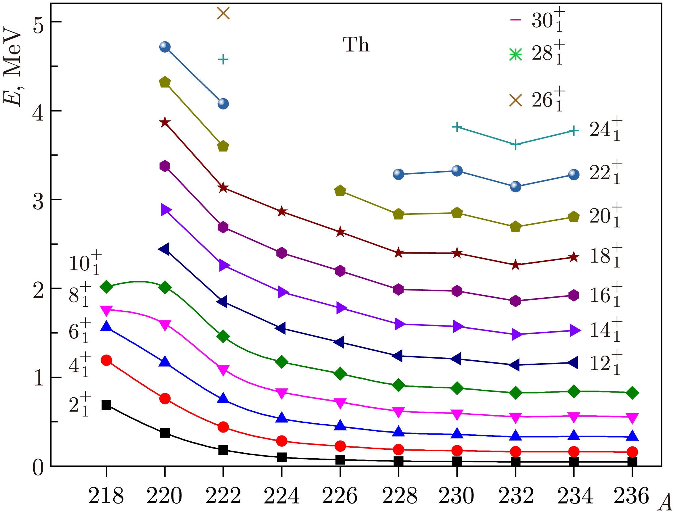

Figure 1.  (color online) Energies of states of the yrast band in even isotopes of thorium

In Fig. 2, for all even thorium isotopes considered, the effective moments of inertia obtained from the experimental and calculated energies in the variable moment of inertia model, designated as Harr, are compared. For two nuclei, ^220,222Th, the results of calculations in the IBM microscopic version, extended by high-spin excitation modes up to spins $ 14^+ $, are also given and is designated as IBM-qp. The parameters determining the values of the moments of inertia are given in Table 1, where the standard deviations of the calculated values of energies from the experimental ones are also given relative to the states for which the parameters were selected, the spins of the states to which the parameters were selected, and the maximum spin in the band. For the ²²⁶Th nucleus, the results of calculations within the framework of the IBM phenomenology are also presented. IBM parameters are given in Table 6.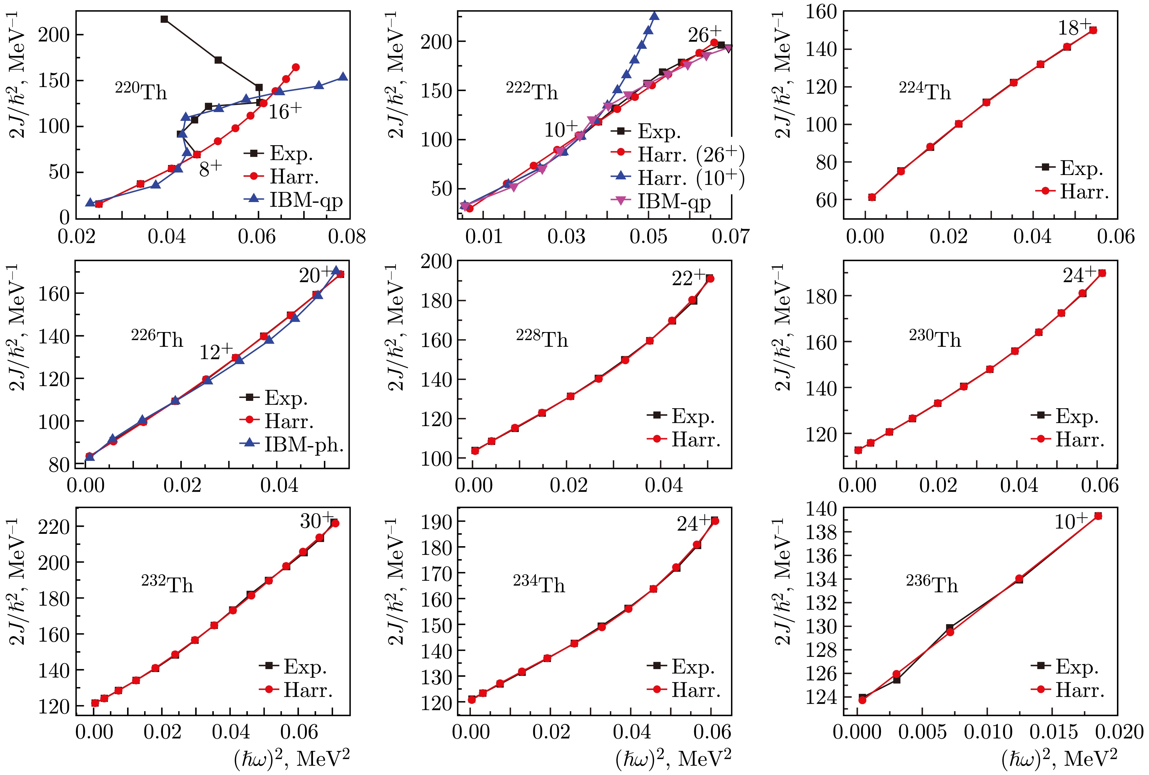

Figure 2.  (color online) Effective moments of inertia from experimental and theoretical energy values of yrast bands in Th isotopes

Nucleus	$ 2J_0/\hbar^2 $	$ 2J_1/\hbar^4 $,	$ 2J_2/\hbar^6 $	$ 2J_3/\hbar^8 $	σ	$ I_{\rm{fit}} $	$ I_{\rm{max}} $
	MeV-1	MeV-3	MeV-5	MeV-7	keV
220Th	-78.027	5627.16	-100806	1032727	0.14E-02	8	22
222Th	11.116	2788.26	865.45	0	9.59	26	26
	17.465	3172.00	-85959.8	1995659.8	0.172	10	26
224Th	57.965	2058.09	-7175.0	9656.4	0.33	18	18
226Th	82.233	1369.23	4017.6	15137.6	0.33	20	20
228Th	102.731	1474.68	-12333.3	349536.8	0.59	22	22
230Th	112.141	1038.92	-2054.2	94199.8	0.175	24	24
232Th	121.107	928.66	10424.0	-50092.3	0.89	30	30
234Th	120.341	984.69	-10471.4	212984.7	0.63	24	24
236Th	123.400	844.93	772.3	0	0.18	10	10
226U	71.87581	1598.41785	6953.44873	-118350.98438	0.294	14	14
230U	115.33965	1119.44153	-3171.23999	121410.60156	0.262	22	22
232U	125.72275	944.34747	3252.86279	64539.00781	0.124	20	20
234U	137.59946	1030.29688	14549.98926	-126356.42969	0.35	30	30
236U	133.45268	385.92599	19432.23242	-89088.77344	1.90	30	30
236U	132.30104	781.21796	-1048.02319	172107.54688	0.155	24	30
238U	133.00563	941.80017	-9015.27832	267665.18750	0.468	28	34
240U	132.39108	388.02209	14673.71387	0.00000	0.413	12	12

Table 1.  Parameters determining the effective moments of inertia for Th and U isotopes

Nucleus	$ \varepsilon_d $	$ k_1 $	$ k_2 $	$ C_0 $	$ C_2 $	$ C_4 $	Ω
226Th	0.367969	-0.030993	0.003373	-0.080729	-0.022919	-0.035625	28
226U	$ -0.080461 $	$ -0.030253 $	$ 0.009227 $	$ 0.005134 $	$ 0.060668 $	$ 0.001103 $	20
226U	$ 0.036599 $	$ -0.038003 $	$ 0.004841 $	$ -0.010224 $	$ 0.033211 $	$ -0.034492 $	28
226U	$ 0.040505 $	$ -0.036817 $	$ 0.004122 $	$ 0.136447 $	$ 0.035798 $	$ -0.031713 $	34
226U	$ -0.059896 $	$ -0.037406 $	$ 0.004168 $	$ 0.001010 $	$ 0.011875 $	$ -0.020448 $	25
230U	$ -0.614828 $	$ -0.058595 $	$ 0.032967 $	$ 0.899961 $	$ 0.061097 $	$ 0.045202 $	21
232U	$ -0.725962 $	$ -0.058227 $	$ 0.032505 $	$ 0.739341 $	$ 0.034253 $	$ 0.054798 $	19
234U	$ -0.594347 $	$ -0.049232 $	$ 0.032013 $	$ 0.674469 $	$ 0.076536 $	$ 0.039112 $	22
234U	$ -0.580119 $	$ -0.049519 $	$ 0.034100 $	$ 0.637994 $	$ 0.071404 $	$ 0.038430 $	21
236U	$ -0.626829 $	$ -0.059598 $	$ 0.051147 $	$ 0.713640 $	$ 0.042979 $	$ 0.019237 $	25
238U	$ -0.634858 $	$ -0.060349 $	$ 0.053701 $	$ 0.687343 $	$ 0.039218 $	$ 0.016058 $	25
240U	$ -0.634453 $	$ -0.059500 $	$ 0.050521 $	$ 0.717118 $	$ 0.029825 $	$ 0.022396 $	25

Table 6.  IBM Hamiltonian parameters for ²²⁶Th even U nuclei

For the lightest of the thorium isotopes under consideration, ²²⁰Th, backbending is observed starting from spin $ 10^+ $, and since the Harris model does not claim to describe it, the parameters were determined from transitions until the state with $ 8^+ $. The energies in ²²⁰Th in the lower part of the spectrum up to spin $ 8^+ $ are perfectly reproduced by the SU(5) limit of IBM. Therefore, these states have no relation to the rotation of the deformed core. This corresponds to the negative value of the parameter $ J_0 $ in Table 1. Nevertheless, the representation of the energies of collective bands through moments of inertia is very convenient in these cases also. In the following isotopes, this parameter is positive and as the collectivity increases, i.e., as the energy of the states decreases, $ J_0 $ increases. In this case, in the theory that explicitly considers the elementary modes of two-quasiparticle excitations with high spins [4, 16], the behavior of the moment of inertia associated with the first backward bend is reproduced. This is demonstrated in Fig. 2 associated with this nucleus. Figure 3 shows the composition of wave functions, whose components include collective states constructed only from d bosons corresponding to the lowest quadrupole excitations, as well as components including bosons $ {\bf{b_J}} $ with high multipolarities. In Fig. 3 and the following one for ²²²Th, the only component with $ b_8 $ that makes noticeable contributions to the wave functions of states, in addition to the collective one determined only by d bosons, is the component with $ b_8 $. There is no direct channel for the interaction of collective states with those containing the $ b_8 $ boson. The interaction is realized through the components with $ b_J $, $ J=2,4,6 $. The latter components contribute to the renormalization of the traditional IBM Hamiltonian. It is for thorium isotopes that only two components were distinguished in the boson representation. If the wave function were represented in terms of D and B phonons, the component with only D phonons would be smaller, and the components with $ B_4 $ and $ B_6 $ phonons would be significant. It should be emphasized that in the presented calculations, the strong indirect interaction of the two components weakly depends on a reasonable change in the position of the $ B_8 $ phonon energy. According to this figure, for the $ 8^+ $ state, the collective component composed only of d bosons is greater than 50%. The second backbending, corresponding to the $ 18^+ $ spin, should be attributed to the four-quasiparticle excitation.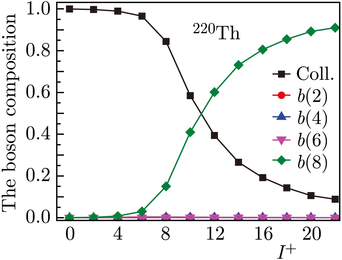

Figure 3.  (color online) The composition of the wave functions of the states of the yrast band obtained on the basis of the microscopic model for ²²⁰Th

For the ²²²Th isotope, no manifestation of the bands crossing is observed. However, the average discrepancy between the calculated energies within the Harris scheme and the experimental ones is significantly larger than for heavier thorium isotopes, as follows from Table 1. The reason for this is that although no backbending is observed in this nucleus, a smooth crossing of bands still occurs, as was shown in [4]. This is demonstrated in Fig. 2, corresponding to ²²²Th, where the moments of inertia obtained on the basis of microscopic calculation are also given. Figure 4 shows the composition of the wave functions. According to this figure, for the $ 12^+ $ state, $ \psi^2 $(coll) is approximately equal to 50%. Therefore, according to the Harris method, in addition to calculations for all energy differences up to the state with spin $ 26^+ $, calculations were made taking into account the states up to the state with spin $ 10^+ $. In the first case, the difference between the calculated and experimental values up to spin $ 8^+ $ is less than 1 keV, and for $ 10^+ $, it is already 5.5 keV. In the second case, this difference for $ 2^+,\ 4^+ $ is about 2 keV, but for the rest, up to $ 14^+ $, it is less than 1 keV. Together with the previous thorium isotope, this shows that the Harris energy calculation procedure can be successfully applied if the collective component in the wave function is definitely greater than 50%.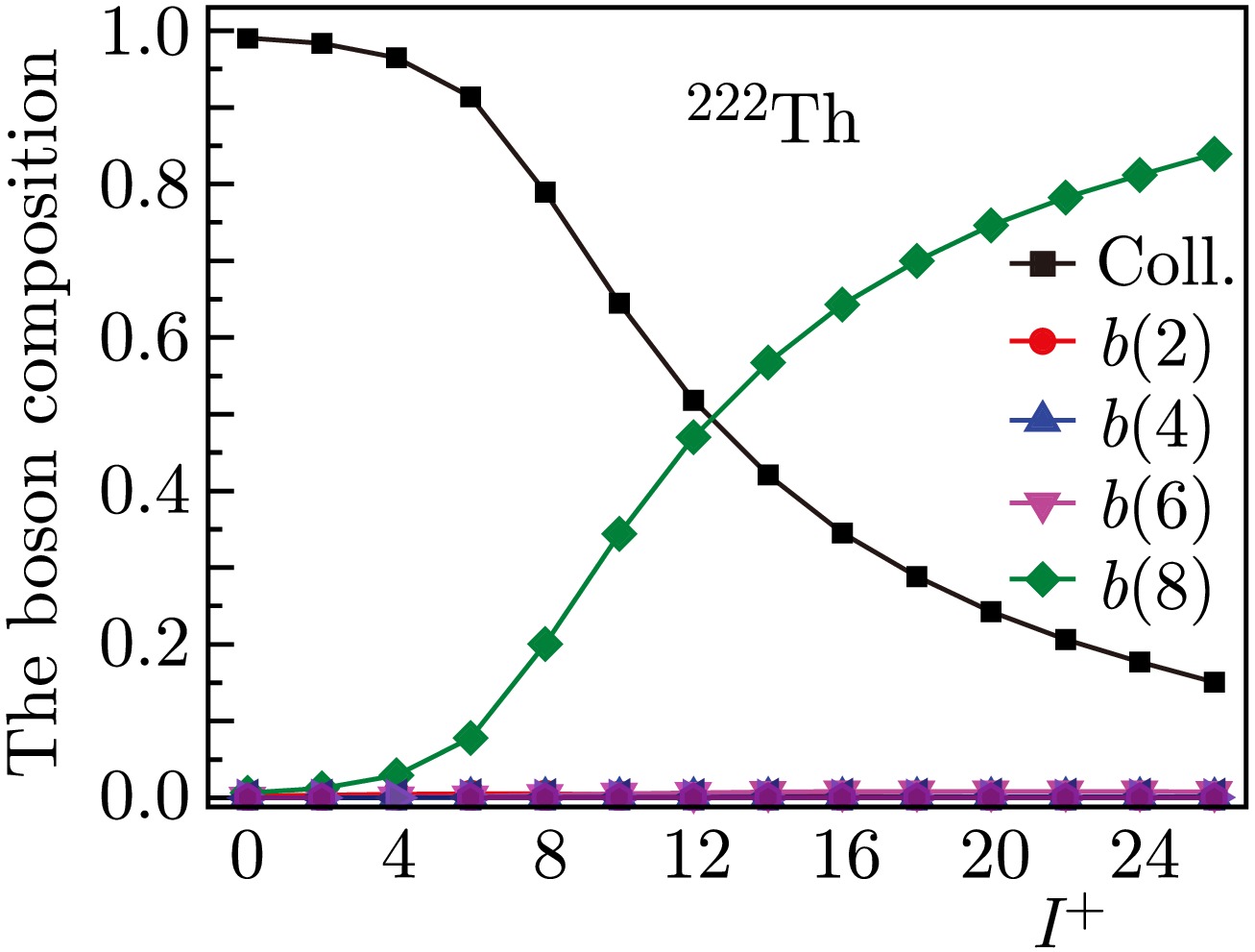

Figure 4.  (color online) The composition of the wave functions of the states of the yrast band obtained on the basis of the microscopic model for ²²²Th

For all nuclei, starting with ²²⁴Th, in the Harris scheme it is achieved such an accuracy of reproduction of experimental energies that the difference between the calculated energies and the experimental ones does not exceed 1 keV on average, as can be seen from the σ values given in the same Table 1. This corresponds to the work [4], where it was found that in thorium isotopes, starting with this one, in all observed states of yrast bands, the collective component remains the main component. The calculated energies obtained in the Harris scheme in Tables 2-5, 9-15 are designated as $ E_{\rm{calc}} $. Table 2 presents the experimental energies of states and the difference between the calculated and experimental energies for ^220-224Th. For ^{226, 228}Th nuclei, a comparison of the experimental and calculated ones is given in Table 3, for ^{230, 232}Th — in Table 4, for ^{234, 236}Th — in Table 5. In almost all of these nuclei, the difference between the calculated energies and the experimental ones does not exceed 1 keV, and for the ^{224, 236}Th nuclei, the calculated energy values differ from the experimental ones by a smaller amount than the experimental errors. Therefore, anomalies in the behavior of $ J(\omega^2) $ for ²³⁶Th in Fig. 2 should be attributed to the experimental errors. This anomaly will disappear if the experimental value $ E(4^+)=160 $ keV is reduced by a value from 0.358 to 0.37 keV. Such a high quality of description of the energies of states in the model of variable moment of inertia in heavy nuclei is achieved given that excitation energies can reach up to 5 MeV, and the spin of states — up to $ 30^+ $.

$ I^\pi $	220Th			222Th			224Th
	exp.	$ E_{\rm{cal}}-E_{\rm{exp}} $		exp.	$ E_{\rm{cal}}-E_{\rm{exp}} $		exp.	$ E_{\rm{cal}}-E_{\rm{exp}} $
$ 2^+ $	$ 386.5(1) $	$ -0.001 $		$ 182.9(2) $	$ -0.06 $		$ 98.1(3) $	$ -0.12 $
$ 4^+ $	$ 759.80(15) $	$ 0.002 $		$ 439.2(3) $	$ 0.22 $		$ 284.1(5) $	$ 0.58 $
$ 6^+ $	$ 1166.03(17) $	$ -0.002 $		$ 749.3(4) $	$ -0.29 $		$ 534.7(5) $	$ -0.30 $
$ 8^+ $	$ 1598.16(20) $	$ -0.0005 $		$ 1092.8(5) $	$ 0.09 $		$ 833.9(6) $	$ -0.46 $
$ 10^+ $	$ 2012.73(23) $	38		$ 1460.8(5) $	$ -0.01 $		$ 1173.8(6) $	$ -0.01 $
$ 12^+ $	$ 2441.9(3) $	78		$ 1850.6(5) $	$ -3.8 $		$ 1549.8(6) $	$ 0.43 $
$ 14^+ $	$ 2885.0(3) $	118		$ 2259.7(6) $	−12		$ 1958.9(7) $	$ 0.21 $
$ 16^+ $	$ 3376.4(6) $	121		$ 2688.0(6) $	−28		$ 2398.0(7) $	$ -0.27 $
$ 18^+ $	$ 3867.1(6) $	136		$ 3133.9(6) $	−51		2864	$ 0.01 $
$ 20^+ $	$ 4319.6(7) $	198		$ 3596.8(7) $	−82
$ 22^+ $	$ 4716.1(12) $	324		$ 4078.6(7) $	−124
$ 24^+ $				$ 4579.2(7) $	−177
$ 26^+ $				$ 5099.2(9) $	−244

Table 2.  Comparison of experimental [17] and theoretical energy values in keV for ^220,222,224Th nuclei

$ I^\pi $	234Th			236Th
	exp.	$ E_{\rm{cal}}-E_{\rm{exp}} $		exp.	$ E_{\rm{cal}}-E_{\rm{exp}} $
$ 2^+ $	$ 49.55(6) $	$ 0.14 $		$ 48.4(3) $	$ 0.09 $
$ 4^+ $	$ 163.05(12) $	$ 0.14 $		$ 160.0(6) $	$ -0.36 $
$ 6^+ $	$ 336.45(24) $	$ -.24 $		$ 329.4(7) $	$ 0.14 $
$ 8^+ $	$ 564.7(3) $	$ -0.80 $		$ 553.4(7) $	$ -0.06 $
$ 10^+ $	$ 842.5(4) $	$ -1.03 $		$ 826.1(9) $	$ -0.04 $
$ 12^+ $	$ 1164.9(6) $	$ -0.81 $
$ 14^+ $	$ 1526.6(7) $	$ 0.11 $
$ 16^+ $	$ 1923.4(8) $	$ 0.80 $
$ 18^+ $	$ 2351.0(9) $	$ 0.72 $
$ 20^+ $	$ 2805.1(11) $	$ -0.13 $
$ 22^+ $	$ 3281.4(12) $	$ -1.04 $
$ 24^+ $	$ 3775.1(13) $	$ -0.15 $

Table 5.  Comparison of experimental [17] and theoretical energy values in keV for ^234,236Th nuclei

$ I^\pi $	226U
	exp.	$ E_{\rm{cal}} $	$ E_{\rm{cal}}-E_{\rm{exp}} $	$ E_{\rm{IBM}} $	$ E_{\rm{IBM}}-E_{\rm{exp}} $
$ 2^+ $	81.3(6)	81.464	0.16	81.510	0.21
$ 4^+ $	250.0(9)	249.682	−0.32	248.46	−1.54
$ 6^+ $	483.2(9)	482.79	−0.41	482.24	−0.92
$ 8^+ $	766.4(10)	766.51	0.11	768.45	2.05
$ 10^+ $	1091.6(10)	1091.98	0.38	1095.9	4.3
$ 12^+ $	1453.8(10)	1453.42	−0.38	1455.7	1.9
$ 14^+ $	1847.0(13)	1846.93	−0.07	1840.1	−6.9

Table 9.  Comparison of experimental [17] and theoretical energy values in keV for ²²⁶U nuclei; for IBM, $ \Omega=20 $

$ I^\pi $	230U
	exp.	$ E_{\rm{cal}} $	$ E_{\rm{cal}}-E_{\rm{exp}} $	$ E_{\rm{IBM}} $	$ E_{\rm{IBM}}-E_{\rm{exp}} $
$ 2^+ $	51.737(23)	51.797	0.060	51.623	−0.114
$ 4^+ $	169.35(4)	169.356	0.006	169.17	−0.18
$ 6^+ $	346.96(20)	346.85	−0.11	347.04	0.08
$ 8^+ $	578.1(3)	577.76	−0.34	578.59	0.49
$ 10^+ $	856.3(3)	855.91	−0.39	857.24	0.94
$ 12^+ $	1175.6(4)	1175.68	0.08	1177.0	1.40
$ 14^+ $	1531.5(4)	1532.07	0.57	1532.7	1.20
$ 16^+ $	1921.0(5)	1920.65	−0.35	1920.1	−0.90
$ 18^+ $	2337.6(6)	2337.56	−0.04	2335.9	−1.7
$ 20^+ $	2779.6(11)	2779.47	−0.13	2777.6	−2.0
$ 22^+ $	3243.6(15)	3243.54	−0.06	3243.7	0.1

Table 10.  Comparison of experimental [17] and theoretical energy values in keV for ²³⁰U nuclei; for IBM, $ \Omega=21 $

$ I^\pi $	232U
	exp.	$ E_{\rm{cal}} $	$ E_{\rm{cal}}-E_{\rm{exp}} $	$ E_{\rm{IBM}} $	$ E_{\rm{IBM}}-E_{\rm{exp}} $
$ 2^+ $	47.573(8)	47.590	0.017	47.533	−0.04
$ 4^+ $	156.566(10)	156.545	−0.021	156.49	−0.076
$ 6^+ $	322.69(7)	322.76	0.065	322.80	0.11
$ 8^+ $	541.1(1)	540.97	−0.13	541.23	0.13
$ 10^+ $	805.88(16)	805.68	−0.20	806.16	0.28
$ 12^+ $	1111.6(2)	1111.59	−0.01	1112.1	0.50
$ 14^+ $	1453.8(3)	1453.91	0.10	1454.1	0.30
$ 16^+ $	1828.2(4)	1828.39	0.19	1828.0	−0.20
$ 18^+ $	2231.6(6)	2231.39	−0.21	2230.4	−1.2
$ 20^+ $	2659.8(9)	2659.78	−0.02	2659.3	−0.5

Table 11.  Comparison of experimental [17] and theoretical energy values in keV for ²³²U nuclei; for IBM, $ \Omega=19 $

$ I^\pi $	234U
	exp.	$ E_{\rm{cal}} $	$ E_{\rm{cal}}-E_{\rm{exp}} $	$ E_{\rm{IBM}} $	$ E_{\rm{IBM}}-E_{\rm{exp}} $
$ 2^+ $	43.4981(10)	43.501	0.003	43.517	−0.195
$ 4^+ $	143.352(4)	143.362	0.010	143.34	1.92
$ 6^+ $	296.072(4)	296.12	0.046	295.89	0.97
$ 8^+ $	497.04(3)	497.06	0.02	496.63	0.17
$ 10^+ $	741.2(5)	741.13	−0.07	740.75	0.54
$ 12^+ $	1023.8(7)	1023.56	−0.24	1023.6	0.60
$ 14^+ $	1340.5(12)	1340.22	−0.28	1340.9	1.50
$ 16^+ $	1687.8(16)	1687.70	−0.1	1689.1	1.90
$ 18^+ $	2062.8(17)	2063.20	0.4	2064.9	2.20
$ 20^+ $	2464.0(18)	2464.49	0.49	2465.9	2.30
$ 22^+ $	2889.5(18)	2889.78	0.28	2890.3	2.0
$ 24^+ $	3338.5(21)	3337.64	−0.86	3336.9	1.9
$ 26^+ $	3807.5(23)	3806.98	−0.52	3805.0	3.2
$ 28^+ $	4296.5(25)	4296.95	0.45	4294.8	3.2
$ 30^+ $	4807	4806.98	−0.02	4807.1	3.2

Table 12.  Comparison of experimental [17] and theoretical energy values in keV for ²³⁴U nuclei; for IBM, $ \Omega=21 $

$ I^\pi $	236U
	exp.	$ E_{\rm{cal}} $	$ E_{\rm{cal}}-E_{\rm{exp}} $	$ E_{\rm{IBM}} $	$ E_{\rm{IBM}}-E_{\rm{exp}} $
$ 2^+ $	45.2431(20)	44.915	−0.33	45.204	−0.0391
$ 4^+ $	149.480(5)	148.921	−0.56	149.43	−0.05
$ 6^+ $	309.788(6)	309.85	0.062	309.87	0.082
$ 8^+ $	522.26(4)	523.77	1.5	522.58	0.32
$ 10^+ $	782.4(5)	785.39	2.99	782.93	0.53
$ 12^+ $	1085.4(7)	1088.97	3.6	1086.0	0.6
$ 14^+ $	1426.4(9)	1429.25	2.8	1426.8	0.4
$ 16^+ $	1801.0(10)	1801.74	0.74	1800.8	−0.2
$ 18^+ $	2204.0(12)	2202.78	−1.2	2203.7	−0.3
$ 20^+ $	2631.8(13)	2629.43	−2.4	2631.7	−0.1
$ 22^+ $	3081.0(14)	3079.34	−1.7	3081.9	0.9
$ 24^+ $	3550.0(17)	3550.57	0.57	3552.0	2.0
$ 26^+ $	4039.0(20)	4041.55	2.6	4040.9	1.9
$ 28^+ $	4549.0(22)	4550.99	1.99	4548.4	−0.6
$ 30^+ $	5077(4)	5077.80	0.8	5075.8	−1.2

Table 13.  Comparison of experimental [17] and theoretical energy values in keV for ²³⁶U nuclei; for IBM, $ \Omega=25 $

$ I^\pi $	238U
	exp.	$ E_{\rm{cal}} $	$ E_{\rm{cal}}-E_{\rm{exp}} $	$ E_{\rm{IBM}} $	$ E_{\rm{IBM}}-E_{\rm{exp}} $
$ 2^+ $	44.916(13)	45.004	0.0883	44.785	−0.131
$ 4^+ $	148.38(3)	148.394	0.014	148.10	−0.28
$ 6^+ $	307.18(8)	307.12	−0.057	307.26	0.08
$ 8^+ $	518.1(3)	517.45	−0.65	518.49	0.31
$ 10^+ $	775.9(4)	775.32	−0.58	777.25	1.35
$ 12^+ $	1076.7(5)	1076.38	−0.32	1078.7	2.0
$ 14^+ $	1415.5(6)	1415.94	0.44	1417.9	2.4
$ 16^+ $	1788.4(6)	1789.15	0.75	1790.1	1.7
$ 18^+ $	2191.1(7)	2191.41	0.31	2191.0	−0.1
$ 20^+ $	2619.1(8)	2618.62	−0.48	2616.7	−2.4
$ 22^+ $	3068.1(9)	3067.34	−0.76	3064.1	−4.1
$ 24^+ $	3535.3(12)	3534.76	−0.54	3530.7	−4.6
$ 26^+ $	4018.1(16)	4018.57	0.47	4015.1	−3.0
$ 28^+ $	4517	4516.92	−0.084	4517.1	0.1
$ 30^+ $	5035.1(21)	5028.27	−6.83	5038.0	2.9
$ 32^+ $	5581(3)	5551.37	−29.6	5580.7	−0.3
$ 34^+ $	6146(4)	6085.16	−60.8	6149.9	3.9

Table 14.  Comparison of experimental [17] and theoretical energy values in keV for ²³⁸U nuclei; for IBM, $ \Omega=25 $

$ I^\pi $	240U
	exp.	$ E_{\rm{cal}} $	$ E_{\rm{cal}}-E_{\rm{exp}} $	$ E_{\rm{IBM}} $	$ E_{\rm{IBM}}-E_{\rm{exp}} $
$ 2^+ $	45(1)	45.274	0.27	45.599	0.6
$ 4^+ $	150.60(10)	150.112	−0.49	150.80	0.2
$ 6^+ $	313.19(14)	312.41	−0.78	312.91	−0.28
$ 8^+ $	528.69(18)	528.43	−0.26	528.12	−0.57
$ 10^+ $	792.9(3)	793.00	0.1	791.95	−0.95
$ 12^+ $	1100.5(4)	1100.32	−0.18	1099.6	−0.9

Table 15.  Comparison of experimental [17] and theoretical energy values in keV for ²⁴⁰U nuclei; for IBM, $ \Omega=25 $

$ I^\pi $	226Th			228Th
	exp.	$ E_{\rm{cal}}-E_{\rm{exp}} $		exp.	$ E_{\rm{cal}}-E_{\rm{exp}} $
$ 2^+ $	$ 72.20(4) $	$ -0.27 $		57.773(3)	$ 0.17 $
$ 4^+ $	$ 226.43(5) $	$ 0.36 $		$ 186.838(3) $	$ 0.08 $
$ 6^+ $	$ 447.3(2) $	$ 0.69 $		$ 378.195(12) $	$ -0.46 $
$ 8^+ $	$ 721.9(2) $	$ 0.38 $		$ 622.5(3) $	$ -0.85 $
$ 10^+ $	$ 1040.3(3) $	$ -0.10 $		911.8(3)	$ -0.78 $
$ 12^+ $	$ 1395.2(4) $	$ -0.24 $		1239.3(4)	$ -0.21 $
$ 14^+ $	$ 1781.5(5) $	$ 0.02 $		1599.4(5)	$ 0.55 $
$ 16^+ $	$ 2195.8(6) $	$ 0.22 $		1987.9(6)	$ 0.64 $
$ 18^+ $	$ 2635.1(7) $	$ 0.32 $		2400.5(8)	$ 0.23 $
$ 20^+ $	$ 3097.1(8) $	$ 0.15 $		2834.4	$ -1.2 $
$ 22^+ $				3283.4	$ -0.15 $

Table 3.  Comparison of experimental [17] and theoretical energy values in keV for ^,228Th nuclei

$ I^\pi $	230Th			232Th
	exp.	$ E_{\rm{cal}}-E_{\rm{exp}} $		exp.	$ E_{\rm{cal}}-E_{\rm{exp}} $
$ 2^+ $	$ 53.230(11) $	$ 0.04 $		49.369(9)	$ 0.02 $
$ 4^+ $	$ 174.119(17) $	$ 0.019 $		162.12(2)	$ 0.08 $
$ 6^+ $	$ 356.54(12) $	$ 0.01 $		333.26(8)	$ 0.29 $
$ 8^+ $	$ 593.89(17) $	$ -0.27 $		556.9(1)	$ 0.23 $
$ 10^+ $	$ 879.36(24) $	$ -0.39 $		826.8(1)	$ -0.22 $
$ 12^+ $	$ 1206.7(5) $	$ 0.06 $		1137.1(5)	$ -0.95 $
$ 14^+ $	$ 1571.9(6) $	$ -0.05 $		1482.2(6)	$ -1.1 $
$ 16^+ $	$ 1969.6(7) $	$ 0.13 $		1858.5(7)	$ -1.2 $
$ 18^+ $	$ 2396.4(9) $	$ 0.09 $		2262.4(9)	$ -0.56 $
$ 20^+ $	$ 2848.7(10) $	$ 0.09 $		2691(1)	$ 0.95 $
$ 22^+ $	3324.1(11)	$ -0.32 $		3144(1)	$ 1.5 $
$ 24^+ $	3819.1(15)	$ -0.05 $		3620.0(15)	$ 0.89 $
$ 26^+ $				4117(2)	$ -0.50 $
$ 28^+ $				4633(2)	$ -1.8 $
$ 30^+ $				5164(3)	$ -0.15 $

Table 4.  Comparison of experimental [17] and theoretical energy values in keV for ^230,232Th nuclei

Heavy nuclei in the majority have a stable deformation, and the deviation to the smaller side of the energies in the band from the dependence $ I(I+1) $ has a number of reasons, partly discussed earlier. This corresponds to the growth of the moment of inertia from the rotation frequency. The monotony of such a dependence at sufficiently large spins of states can be violated, leading, for example, to backbending, and this invariably occurs in medium nuclei. Also, an anomaly in the behavior of the moment of inertia can manifest itself through upbending, when the intersection of bands is not fully completed. And finally, downbending. This effect can manifest itself at spins of at least $ 26^+ $ and in those cases when, for example, a state with the same spin, but in the S band, turns out to be significantly higher and the observed state remains mainly collective. Moreover, the energies of such high-spin collective states may turn out to be somewhat higher than those that would be obtained based on the trends corresponding to lower spins. There may be two reasons for such a behavior of the energies of collective states at high spins. One is associated with the reduction of the configuration space of two-quasiparticle states that form the D phonon, in the presence of multibosons, which is realized to a greater extent at high spins. To quantitatively evaluate this phenomenon at the energy of collective states, it is necessary to carry out self-consistent solutions for each of the collective states separately, as was done for medium nuclei [9]. However, for heavy nuclei, such a procedure is difficult to implement due to the high sensitivity of the calculated energies to the IBM Hamiltonian parameters. Another reason for some additional growth of energies of collective states at high spins, which is what downbending gives, may be the specificity of the description of collective states in the general case of the $ SU(6) $ symmetry, which consists in the finiteness of the maximum number of quadrupole bosons Ω.

In the variable moment of inertia model, the growth of the slope $ J(\omega^2) $ is effectively reproduced. One of the reasons for this growth is the gradual increase of the noncollective component in the states of the yrast band. This explains why in deformed nuclei the quality of the description of energies in the Harris model is better than in the IBM phenomenology. The situation regarding IBM changes if we move from its phenomenology to the microscopic version, when the IBM parameters are calculated and high-spin excitation modes are explicitly taken into account. This also allows us to determine the limits of applicability of the Harris scheme in the region of spins where the bands cross. For example, a microscopic calculation of the structure of the states of the yrast band in ²²²Th showed [4] that the Harris scheme successfully reproduces collective states in which the collective component is noticeably larger than any of the others, and itself can be somewhat less than 50%.

The parameters determining the moment of inertia for U isotopes are given in Table 1. The corresponding moments of inertia are given in Fig. 5. In addition to the experimental and calculated values of the moments of inertia according to Harris, the results of calculations in accordance with the IBM phenomenology are given, excluding high-spin modes.

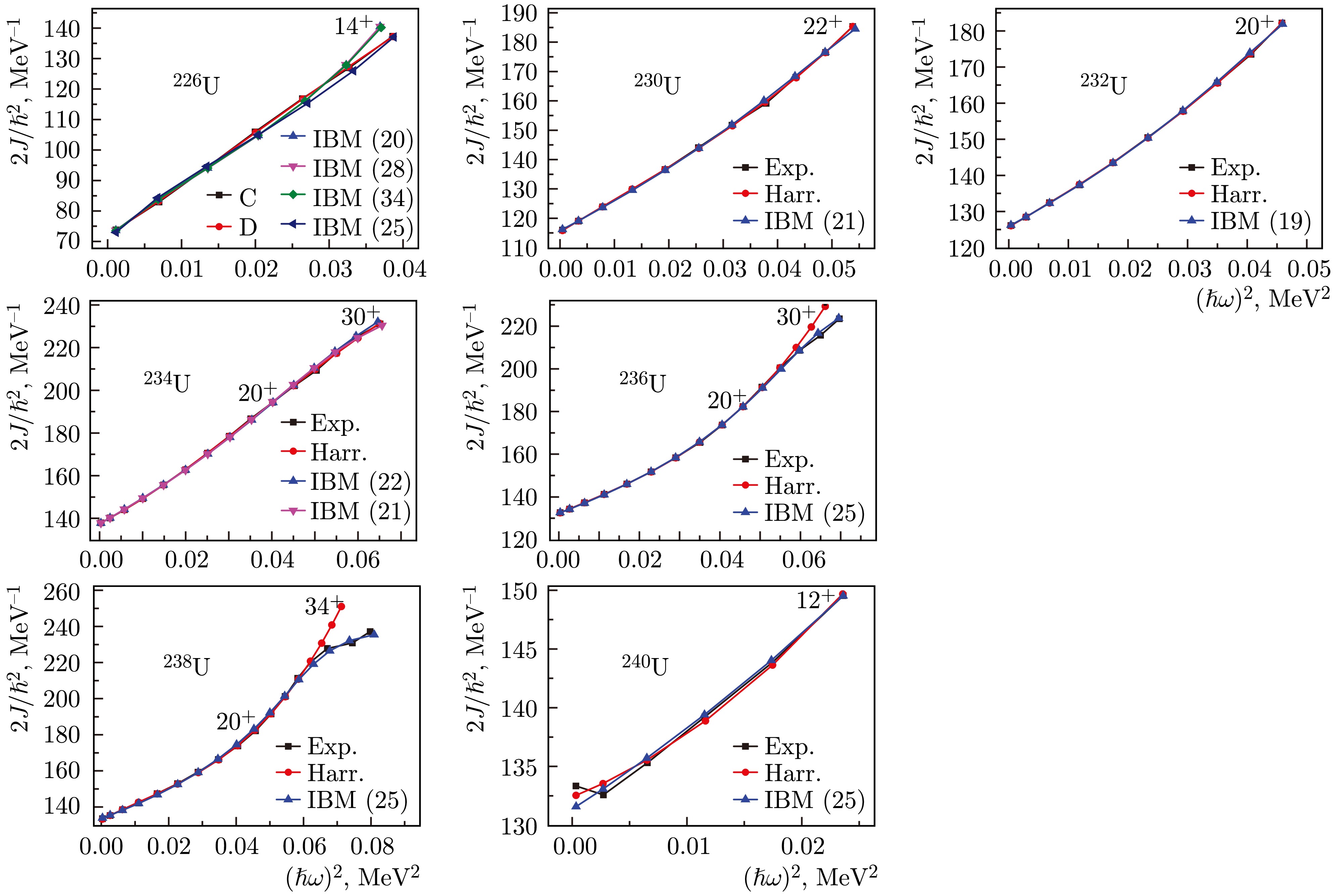
Figure 5.  (color online) Effective moments of inertia from experimental and theoretical energy values of yrast bands in U isotopes

The parameters of the boson Hamiltonian (8) for the U isotopes are given in Table 6 and the corresponding moments of inertia with others are also given in Fig. 5. The parameters of the boson Hamiltonian given in Table 6 are given with an accuracy of 1 eV. To justify the need for such high accuracy, the partial derivatives $ {\partial E_I}/{\partial\varepsilon_d}, \ldots, {\partial E_I}/{\partial C_4} $ were calculated in the vicinity of the parameter values determined for ²³⁶U. They are given in Table 7. In accordance with these values, the maximum deviations of the parameters were obtained when the deviations of the calculated energies do not exceed 0.1 keV. These values are given in Table 8. The change in the Hamiltonian parameter (8) $ k_1 $ reacts most strongly to the energies of the states under consideration. And as can be seen from Table 8, at high spins its values should be given with greater accuracy than 1 eV, but since at high spins the experimental uncertainty of energies exceeds 1 keV, this can be avoided for now.

$ I^\pi $	$ 0^+ $	$ 2^+ $	$ 4^+ $	$ 6^+ $	$ 8^+ $	$ 10^+ $	$ 12^+ $	$ 14^+ $	$ 16^+ $	$ 18^+ $	$ 20^+ $	$ 22^+ $	$ 24^+ $	$ 26^+ $	$ 28^+ $	$ 30^+ $
$ {\partial E_I}/{\partial\varepsilon_d} $	11	$ 0.071 $	$ 0.23 $	$ 0.48 $	$ 0.8 $	$ 1.2 $	$ 1.7 $	$ 2.2 $	$ 2.7 $	$ 3.3 $	$ 4.0 $	$ 4.7 $	$ 5.4 $	$ 6.2 $	$ 6.9 $	$ 7.7 $
$ {\partial E_I}/{\partial k_1} $	316	$ -2.5 $	$ -8.1 $	$ -16.7 $	−28	$ -41.7 $	$ -57.4 $	$ -74.8 $	$ -93.7 $	−113	−134	−155	−175	−196	−216	−234
$ {\partial E_I}/{\partial k_2} $	−138	$ 0.475 $	$ -1.54 $	$ -3.09 $	$ -5.0 $	$ -7.1 $	$ -9.3 $	$ -11.4 $	$ -13.4 $	−15	−16	$ -16.6 $	$ -16.3 $	$ -15.2 $	−13	$ -9.5 $
$ {\partial E_I}/{\partial C_0} $	12	$ -0.067 $	$ -0.23 $	$ -0.47 $	$ -0.8 $	$ -1.21 $	$ -1.7 $	$ -2.2 $	$ -2.9 $	$ -3.6 $	$ -4.2 $	$ -5.1 $	$ -5.8 $	$ -6.6 $	$ -7.4 $	$ -8.2 $
$ {\partial E_I}/{\partial C_2} $	−17	$ 0.071 $	$ 0.23 $	$ 0.48 $	$ 0.8 $	$ 1.19 $	$ 1.7 $	$ 2.2 $	$ 2.7 $	$ 3.3 $	$ 3.9 $	$ 4.6 $	$ 5.3 $	$ 6.0 $	$ 6.7 $	$ 7.3 $
$ {\partial E_I}/{\partial C_4} $	23	$ 0.65 $	$ 2.16 $	$ 4.55 $	$ 7.8 $	$ 11.9 $	$ 17.0 $	$ 22.9 $	$ 29.6 $	$ 37.4 $	$ 46.0 $	$ 55.6 $	$ 66.2 $	$ 77.7 $	$ 90.2 $	104

Table 7.  Partial derivatives of IBM energies with respect to boson parameters in the special case of parameters adopted for ²³⁶U, $ E_{I\geq 2} $ are understood to be the excitation energy, and $ E_0 $ — the total boson energy, measured from the energy of the d-boson vacuum

$ I^\pi $	$ 0^+ $	$ 2^+ $	$ 4^+ $	$ 6^+ $	$ 8^+ $	$ 10^+ $	$ 12^+ $	$ 14^+ $	$ 16^+ $	$ 18^+ $	$ 20^+ $	$ 22^+ $	$ 24^+ $	$ 26^+ $	$ 28^+ $	$ 30^+ $
$ \triangle\varepsilon_d $	9	1400	430	210	125	83	59	45	37	30	25	21	18	10	14	13
$ \triangle k_1 $	0.32	40	12	6	$ 3.6 $	$ 2.4 $	$ 1.7 $	$ 1.3 $	$ 1.1 $	$ 0.88 $	$ 0.75 $	$ 0.65 $	$ 0.57 $	$ 0.51 $	$ 0.46 $	$ 0.43 $
$ \triangle k_2 $	0.72	210	65	32	20	14	11	$ 8.8 $	$ 7.5 $	$ 6.7 $	$ 6.2 $	$ 6.0 $	$ 6.1 $	$ 6.6 $	$ 7.7 $	10
$ \triangle C_0 $	8	1492	435	213	125	83	59	45	34	28	24	20	17	15	14	12
$ \triangle C_2 $	6	1408	435	208	125	84	59	45	37	30	26	22	19	17	15	14
$ \triangle C_4 $	4	154	46	22	13	$ 8.4 $	$ 5.9 $	$ 4.4 $	$ 3.4 $	$ 2.7 $	$ 2.2 $	$ 1.8 $	$ 1.5 $	$ 1.3 $	$ 1.5 $	$ 1.3 $

Table 8.  The required accuracy of the parameters in eV so that the accuracy of calculating the energy of the yrast band states is not less than 0.1 keV in the particular case of the parameters adopted for ²³⁶U, for $ I\neq 0 $, the energies are considered relative to the ground state

The IBM Hamiltonian parameters, including the Ω number, for ^226-238U were determined from states up to the limiting observed spins and are given in Table 6. Let us discuss the quality of the description of the energies of states consistently in all uranium isotopes under consideration.

For ²²⁶U, the experimental data show a practically linear dependence of $ J(\omega^2) $ and this is naturally reproduced in the Harris scheme. This could not be obtained in the description in IBM. The calculations were carried out in a wide range of Ω from 14 to 34. In this case, if the quality of reproduction of energies for states with $ I\leq 12^+ $ is satisfactory, and this is evident from Table 9, where the values of energies with $ \Omega=20 $ are given, then the energy of the state with $ 14^+ $ turns out to be underestimated by 7 keV, and this leads to the calculated increase in the value of J. If we degrade the quality of the energy description, the linear dependence $ J(\omega^2) $ is approximately reproduced, which is reflected in the corresponding Fig. 5. The question of the possibility of quantitative reproduction of the energies of the ²²⁶U nucleus in IBM remains open. This is despite the fact that the question concerns the description of states up to relatively low spins. It should be borne in mind that the experimental errors for this isotope are the highest of all those considered.

For the next nucleus, ²³⁰U, the description of energies in the Harris scheme is precise and the difference between the calculated and experimental values of energies, as can be seen from Table 10, does not exceed 0.4 keV. Within the IBM framework, this is 1.4 keV, which also indicates a high quality of the description. This is despite the fact that states are observed up to $ 22^+ $.

For ²³²U, states are observed up to $ 20^+ $ and the description of their energies in the two calculations is quite satisfactory. Thus, in the Harris scheme, the discrepancy is no more than 0.21 keV, and for IBM — no more than 1.2 keV, as follows from Table 11. The quality of the energy description is especially clearly manifested through the moments of inertia for ²³⁰U and ²³²U in Fig. 5.

For ²³⁴U, states are observed already up to $ 30^+ $. In the Harris scheme, the discrepancy is no more than 0.86 keV. Within the IBM framework, as can be seen from Fig. 5, calculations were made with two values of Ω, these are 21 and 22. The results of the calculations of the moments of inertia closely cover the moments of inertia from the experimental energies on both sides. Taking into account the influence of high-spin modes on the energies of states, we give preference to $ \Omega=21 $ and it is with this value that the calculated values are presented in Table 12, from which it is clear that the corresponding differences are no more than 3.2 keV.

In the ²³⁶U nucleus, the observed states also extend to $ I=30^+ $. The observed moments of inertia at $ I=28^+ $ and $ I=30^+ $ definitely give a decrease in the slope of $ J(\omega^2) $. More precisely, starting from spin $ 26^+ $, a slower growth of the moment of inertia — downbending — is manifested. That is why the parameters in the Harris scheme were determined by the states up to spin $ I=24^+ $ and for these states, the difference between the experimental and calculated energies does not exceed 0.74 keV, as follows from Table 13. The moments of inertia at high spins, as can be seen from Fig. 5, for this nucleus significantly exceed the experimental values. The calculation in IBM reproduces this experimental trend and this is achieved at $ \Omega=25 $. This can be associated with a decrease in the collective configuration space at the corresponding spins, as well as the presence of s bosons or square roots, due to which the closure of the $ SU(6) $ algebra of boson operators is realized in comparison with other collective models. This is the case when the variable moment of inertia model with the used parameterization cannot describe this phenomenon, and the IBM phenomenology describes the corresponding increase in the energies of collective states. Such a phenomenon is realized, as can be judged by ^{236, 238}U nuclei, starting with spin $ 28^+ $. For all states of this nucleus, the difference between the calculated IBM and experimental energy values does not exceed 2 keV.

The effect observed in the ²³⁶U nucleus of weakening the growth of J from $ \omega^2 $ at $ I=28^+,\ 30^+ $ is even more pronounced in the ²³⁸U nucleus, since the spins observed for it extend to $ I=34^+ $. The parameters in the Harris scheme were determined by the states with $ I\leq 28^+ $ and for these states, as can be seen from Table 14, the difference between the experimental and calculated energies does not exceed 0.76 keV. For large spins, this difference grows rapidly, and the calculated energy values are noticeably lower than the experimental ones. As can be seen from Fig. 5, for this nucleus, the calculation in IBM reproduces the experimental situation and this is realized at $ \Omega=25 $. If we use large values of Ω, for example, 30, then J will be significantly larger, approaching those given by the Harris scheme. The difference between the experimental and calculated energies within the IBM framework for all spins does not exceed 4.6 keV.

It should be noted that the description of the energies of states in a number of uranium nuclei is so good that the discrepancies with experimental values sometimes give smaller values than the experimental uncertainties, especially for calculations in the Harris scheme.

As a rule, the quality of description in the Harris model is higher than in IBM, this is evident from ^{226,230,232,234}U (there are no experimental data for ²²⁸U). This can be explained by the method of determining the parameters. For the Harris scheme, they are determined by the least squares method, which makes them clearly optimal, while for IBM, other methods for determining the parameters have to be used, which are not so effective. For ²³⁶U, as can be seen from Fig. 5, both models reproduce the energies equally qualitatively.

For ²⁴⁰U, states are known only up to spin $ 12^+ $. In Fig. 5, for ²⁴⁰U, a strong anomaly of the moment of inertia for the first excitation is visible. It cannot be reproduced by any of the models and its presence is associated with a large experimental error in the energy of the first excitation (see Table 15). If, when describing energies within the IBM framework, the determination of parameters is carried out without the $ 2^+_1 $ state, then its energy turns out to be equal to 45.6 keV, that is, 0.6 keV higher than that suggested by the experiment. In this case, the experimental error for this state is equal to 1 keV, i.e., such a correction is within the experimental corridor of admissible values, and the anomaly in the effective moment of inertia is the result of a large experimental uncertainty. If the moments of inertia are determined with the corrected energy of the $ 2^+ $ state, the value of σ will decrease significantly and become equal to 0.08.

A comparison of the effective moments of inertia for heavy even nuclei, namely, thorium and uranium isotopes, with the variable moment of inertia model and IBM, both in its phenomenological aspect and in its microscopic version, allowed us to draw the following conclusions.

1. The Harris model effectively reproduces the experimental situation if the collective component in the wave function remains at least 50%. The standard boson model cannot do this; for this, it must be extended by explicitly taking into account high-spin excitation modes up to $ J\leq 14^+ $. However, the Harris scheme does not reproduce the decrease in the slope of J from $ \omega^2 $.

2. If the energies of collective states increase significantly at spins greater than $ 28^+ $, this may be due to a reduction in the collective configuration space. This situation is reproduced in the IBM phenomenology, but cannot be reproduced in either the Harris model or classical geometric collective models.

In this paper, the Harris scheme is not considered through the use of the cracking model, but only as one of the convenient and visual representations of the excitation energies in the bands. In a number of cases for the lowest states, when there are large experimental uncertainties, it can give clarifying estimates. For large values of spins, when the experimental values of the moments of inertia are noticeably greater than the Harris estimates, it is possible to make judgments about the extent of the influence of noncollective modes with high spins on these states.