On the generalized Friedrichs-Lee model with multiple discrete and continuous states

Unstable states constitute a ubiquitous phenomenon in contemporary physics, manifesting across various disciplines such as molecular physics, nuclear physics and particle physics. In the realm of hadronic physics, the prevalence of unstable resonances is particularly notable within the context of strong interactions, where new resonant states are frequently encountered and documented. These resonances assume significant significance in unraveling the fundamental characteristics of hadrons and their interactions, perpetuating their investigation as a vibrant research area within the field of particle physics.

To explore the characteristics of unstable states across diverse branches of physics, several models sharing a similar conceptual framework have independently emerged. Among these models, the Friedrichs model stands as a simple non-relativistic Hamiltonian that couples a bare discrete state to a bare continuous state [1]. Within this model, the solutions for unstable generalized eigenstates can be rigorously obtained and expressed in terms of the bare states. In the realm of quantum field theory, the Lee model was developed to investigate the properties of field renormalization [2]. This model considers two nucleon states, denoted as N and V, which can be converted to each other by absorbing or emitting a bosonic θ particle through the processes $ V\rightleftharpoons N+\theta $. Analogous models can be found in various domains, such as the Jaynes-Cummings model in quantum optics [3] and the Anderson model in condensed matter physics [4]. In this article, we collectively refer to these models as the Friedrichs-Lee (FL) model, highlighting their common conceptual foundation. The generalized eigenstates of the full interacting Hamiltonian within the FL model can be explicitly determined in terms of the original discrete state and the continuum states.

The original Friedrichs-Lee model, which involves only one discrete and one continuous state, is often considered as a toy model due to its simplicity. It is usually employed to comprehend the properties of bound states, virtual states and resonant states that appear in the scattering processes. When the bare discrete state is above the continuum threshold, its pole position moves to the second sheet and become a pair of resonance poles. If the bare discrete state is below the threshold, there would be an accompanied virtual state pole on the second sheet when the interaction is turned on. Besides these states generated from the bare discrete states, there could also be dynamically generated states from the singularities of the interaction vertices [5]. The mathematical background of describing the unstable states is the Rigged Hilbert Space (RHS) quantum mechanics [6−8], rather than the conventional Hilbert space. In the RHS quantum mechanics, the Hamiltonian H, as an Hermitian operator, could have generalized complex eigenvalues and the related eigenstates corresponding to the pole of the S-matrix that lies on the unphysical sheet of the analytically continued energy plane, commonly referred to as the Gamow states. The Friedrichs model was also extended to include more continuous or discrete states and with a more realistic interaction vertex function. As a result, it finds extensive application in a wide range of realistic scenarios, particularly in the study of hadronic scattering processes [9−14]. Furthermore, coupled-channel models sharing similar spirits have demonstrated success in describing a variety of resonance phenomena in different physical systems [15−25]. The widespread applicability and efficacy of these models in describing resonance phenomena render them as powerful tools in studying the properties of unstable states in different physical contexts.

In the hadron physics, the usual effective field theory calculation of the scattering amplitude encounter challenges pertaining to unitarity and analyticity. The perturbative S matrix generally fails to generate bound states or resonance poles on the analytically continued Riemann surface of the energy plane. To address this, various unitarization methods are used, such as the K-matrix method. The typical K-matrix parameterization of the S-matrix like $ S=\dfrac {1-iK}{1+iK} $ lacks a dynamical origin and enforces unitarity by hand. However, this parametrization does not guarantee the absence of unphysical spurious poles, including those situated in the complex energy plane of the first Riemann sheet, which violates causality. In contrast, the Friedrichs-Lee model achieves unitarity as a consequence of its dynamics, and the Hermitian property of the Hamiltonian ensures the absence of spurious poles in the first Riemann sheet. These are the immediate advantages of these kinds of models over the K-matrix parameterization.

While there have been notable achievements in the application of such models, certain aspects still call for further improvement. From a quantum field theory perspective, the previous model only considered the contribution of intermediate s-channel discrete state to the amplitude. However, there are other types of interactions that are not included. The first one comes from the crossed channels in the two-to-two scattering amplitude, where the intermediate particle can also appear as the t- or u-channel propagators. The second one involves the contact interactions, such as the four-point vertex. Upon performing a partial wave projection, both of these interactions can be represented by continuum-continuum interactions. These interactions introduce a mild background to the final experimental observation, potentially interfering with the s-channel resonances and modifying the lineshape. It is crucial to include these background contributions in the analysis of the experimental data while preserving analyticity and unitarity. The commonly used Breit-Wigner parametrization to parameterize the t- or u-channel resonance and a polynomial to parameterize the background would violate the unitarity. A naïve K-matrix unitarization may introduce unexpected spurious poles in the S-matrix. Thus, to incorporate the continuum-continuum interactions into the Friedrichs-Lee like models could overcome these problems. However, a general continuum-continuum interaction renders the model no longer solvable. In refs. [10, 26], a particular form of separable interaction involving the continuum states is introduced, where the interaction vertex function between the discrete states and the continuum also appears as the factors of the separable interaction between two continuum states. The Hamiltonian is

where the form factor $ f_i(\omega) $ is associated with the i-th continuum state $ |\omega;i\rangle $, both for its the interaction with different discrete states and for its interaction with other continuum states. There are two aspects which could be improved for this model. First, the interaction between the discrete states $ |j\rangle $ and the continuum could be extended to a general function $ f_{ij}(\omega) $, for a more realistic description of the strong interaction in the real world. Using the quark pair creation (QPC) model as an example, the interaction between a meson and their decay products is expressed as a complicated integration between the wave function for the three states and the pair production vertex [12, 27]. Thus the form of the interaction function depends both on the discrete state and the continuum. Secondly, the interaction between the continuum states does not need to be factorized using the same factors as the interaction between the discrete state and the continuum. In this paper, we will demonstrate that after factorizing the continuum-continuum interaction independent of the discrete-continuum interaction, the model remains exactly solvable. In principle, the extra continuum-continuum interaction should be the residue interaction after subtracting the s-channel intermediate discrete state contribution, which could have no relation with the discrete-continuum interaction. Whether this interaction can be expressed as a separable potential remains an open question. There are aleady some physical applications of the separable potentials in discussing real world problems, for example, describing the interaction between the open-flavor channels and the hidden-flavor channels in momentum space [?]. Our formalism differs from this implementation by two key advances: First, we parameterize all continuum-continuum couplings via separable potentials, withou the distinction between open-flavor and hidden -flavor channels. This enables a more general description of coupled-channel systems. Secondly, by projecting potentials onto angular momentum eigenstates through spherical harmonic expansion, the three-dimensional momentum integration reduces to a one-dimensional radial integral. This systematically eliminate angular variables, significantly simplifying both numerical implementation and analytical discussion of mementum dynamics. Moreover, in general, a square-integrable interaction potential between continuum states could be expanded using a series of general separable basis. In fact, one can also expand both the discrete-continuum interaction vertex and continuum-continuum interaction vertices using the same function basis. Thus, the study of such separable potentials may have broader physical applications. In this paper, our focus lies on these two kinds of improvements: the incorporation of a more general discrete-continuum interaction and various separable continuum-continuum interactions among multiple bare discrete and continuum states in the FL model. By rigorously solving the eigenstates for the Hamiltonian, we obtain the "in'' and "out'' states, the scattering S-matrix, discrete state solution, and other mathematical physics properties. Our aim is to establish a solid foundation for the further phenomenological applications of the FL model by including these additional physical features.

We organize the paper as follows: In Section II, the solution of the FL model with more general interactions between discrete states and continuum states is derived. Section III discusses the case with extra separable continuum-continuum interactions. Section IV is devoted to studying the case when the interaction potential between continuum states could be approximated by a sum of separable potentials and consider the cases when both the continuum-continuum potential and continuum-discrete potentials are approximated by a truncated series. In section V, as an application, we consider some simple examples and discuss the behavior of the discrete states after turning on various interaction. Section VI is the conclusion.

First, we are going to consider a system with D kinds of discrete states and C kinds of continuum states, where C and D denote the numbers of the continuum states and the discrete states respectively. If there is no interaction, the mass of the j-th discrete state $ |j\rangle $ is $ M_j $, while the energy spectrum of the n-th continuum state ranges in $ [a_n,\infty) $ with the threshold energy $ a_n $. The interaction between the j-th discrete state and the n-th continuum state can be generally represented by a coupling function $ f_{jn}(\omega) $. The full Hamiltonian can be expressed as

where the free Hamiltonian $ H_0 $ could be written down explicitly as

and the interaction part $ H_I $ reads

The free eigenstates are supposed to be orthogonal to each other and the normalization conditions satisfy $ \langle i|j\rangle=\delta_{ij} $, $ \langle i|\omega;n\rangle=0 $ and $ \langle \omega;n|\omega';n'\rangle=\delta(\omega-\omega')\delta_{nn'} $. For simplicity, we first suppose that there is no degenerate threshold and no degenerate discrete states. In fact, if there are degenerate states with the same threshold and the same interactions with the other states, the corresponding solutions will also be degenerate with the same expression after the interactions are turned on, and we will take them as one state with degenerate degrees of freedom just like different magnetic quantum numbers when there is no magnetic field. If the states with degenerate threshold take part in different interactions, the following discussion will not be modified too much. We will come back to this case later.

The general solution for the energy eigenvalue problem $ H|\Psi(E)\rangle=E|\Psi(E)\rangle $ can be represented as a linear combination of the discrete states and the continuum states,

where the $ \alpha_i(E) $ and $ \psi_n(E,\omega) $ functions are defined as the coefficient functions of the discrete states and the continuum states respectively. By substituting this ansatz into the eigenvalue equation, and carefully examining the coefficients preceding the discrete states and the continuum states, we can derive two distinct sets of equations,

An important observation to make is that the formula exhibits a nontrivial complexity, which does not appear in the single-channel scenario. Specifically, for a given energy range $ a_l < \omega < a_{l+1} $, there are only l equations present in Eqs. (7).

Consequently, the eigenvalue problem yields both continuum solutions and discrete solutions. These solutions correspond to different regimes of the spectrum, which will be addressed carefully in the following.

1. The continuum state solutions

When the energy E is above the highest threshold, that means, $ E>a_C $, there will be C continuum states when the interactions are turned on, so the m-th continuum solution will be

However, when the energy E is lower than the highest threshold, e.g., $ E\in[a_l,a_{l+1}) $, $ l<C $, there will be l degenerate continuum eigenstates, $ m=1,2\dots,l $, and the other states are not well-defined below their thresholds and are set to $ \mathbf 0 $. To remove the ambiguity of the degenerate states, it is required that when the interaction is turned off, i.e. $ f_{jm}(\omega)\to 0 $, $ |\Psi_m\rangle $ tends to the free continuum state $ |E;m\rangle $. We expect that, when the eigenvalue $ E\in[a_1,a_2] $, we can solve $ \alpha_{1,i} $ and $ \psi_{1,i} $ in $ |\Psi_1(E)\rangle $, and then analytically extend these parameters to $ E\in[a_2,a_3] $ to solve $ |\Psi_2(E)\rangle $, and so on. In this way the eigenfunctions can be uniquely determined. From Eq. (6,7) in terms of the coefficients in Eq. (8), the coefficient function $ \psi_{mn}(E,\omega) $ before the continuum state in different energy regions could be expressed as

This equation could be concisely written down in one equation by using the Heaviside step function $ \Theta(x) $,

Notice that $ \psi^{\pm}_{mn} $ is a generalized function, and in order to distinguish between different integral contours, we have included $ \pm i0 $ in the denominator of the integral in Eq.(8). The $ \psi^+ $ state corresponds to the coefficient for the in-state while $ \psi^- $ corresponds to those of the out-state. For the convenience of the future discussions, we will omit the superscripts $ \pm $ in the notations. It should be understood that the appropriate superscript can be easily inferred based on the context. In the cases where there is a need to explicitly indicate the in-state or out-state, we will make use of the superscript accordingly.

Inserting this equation back into Eq.(6), we can obtain the equations for the coefficient functions $ \alpha_{mk}(E) $ for $ m=1,2,\dots l $

With many different discrete states and continuum ones involved in, the representation becomes much more complex than the simplest version. In fact, the formula and the derivation procedure could be simplified by introducing the matrix form. In the following, the matrices are represented in bold faces and the dot symbol "$ \cdot $" represents the matrix product, and the matrix element is expressed in the form like $ (\boldsymbol\eta)_{ij} $. For example, Eq. (10) could be written down in the matrix form as

where $ \boldsymbol \alpha $ and $ \mathbf f $ are the $ C\times D $ and $ D\times C $ matrices for the coefficients $ \alpha_{mk} $ and $ f_{jm} $, respectively. The matrix $ \boldsymbol\gamma $ is defined as a diagonal matrix of dimension $ C\times C $

whose diagonal elements $ \gamma_n $ could be different in principle for different n and the values could be determined by the normalization conditions. The $ \boldsymbol\eta_\pm $ matrix, the inverse of resolvent function matrix, is of dimension $ D\times D $ and every matrix element reads

In general, the determinant of η matrix does not vanish for $ a_l<E<a_{l+1} $, and the matrix $ \boldsymbol\alpha^\pm $ can be represented as

Inserting this result into Eq. (9), the coefficient functions $ \psi_{mn} $ before the continuum states can be obtained in matrix representation

The solution of the continuum eigenstate can then be expressed as

Notice that in the energy region $ a_l<E<a_{l+1} $, the wave function $ |\Psi^\pm_m\rangle $ for $ m>l $ should vanish. Another required condition is that, when the coupling function $ f_{jn} $ vanishes, $ |\Psi^\pm_m(E)\rangle $ tends to $ |E,m\rangle $. Therefore, the coefficient $ \gamma_m $ is determined to be 1. It can be checked that the normalization satisfies $ \langle \Psi^\pm_m(E)|\Psi^\pm_n(E')\rangle=\delta(E-E')\delta_{mn} $. Actually, in the point view of the scattering theory, $ |\Psi^+\rangle $ is the "in" state and $ |\Psi^-\rangle $ is the "out" state, so the S matrix can be obtained by inner product of the "in" state and the "out" state as

The $ \boldsymbol\eta_\pm(E) $ function can be analytically extended to the complex E plane with $ \eta_+(E) $ and $ \eta_-(E) $ coinciding with $ \boldsymbol \eta(E) $ on the upper edge and lower edge of the real axis above the thresholds, respectively. We can also define the analytically continued S matrix

where E is analytically continued to the complex energy plane and only when E is real and on the upper edge of the cut above the lowest threshold $ a_1 $ is the S matrix the physical one. Given the presence of C continuous states with distinct thresholds, it is a general result that there exist $ 2^C $ different Riemann sheets for the analytically continued S matrix. Since only the Riemann sheets nearest to the physical region affect the physical S-matrix the most, we label the m-th sheet as the Riemann sheet continued from the physical region $ (a_m,a_{m+1}) $, where the first sheet where the physical S matrix resides is called physical sheet by convention.

It is worth pointing out that the formula of scattering matrix Eq. (14) has important phenomenological applications. For example, in studying the particle-particle scattering processes, the two particles that collides or those final states (usually called as channels in the scattering experiments) form continuum states, while the intermediate resonance states are regarded as the discrete states. The $ (n,m) $-th element of scattering matrix in Eq. (14) could describe the scattering amplitudes from the channel of n-th continuum state to the m-th channel. The coupled-channel unitarity is naturally satisfied among all the related scattering amplitudes due to the obvious relation $ \mathbf S\mathbf S^\dagger= I $. Furthermore, once the coupling function between the discrete and continuum state is reliably described by some dynamical models, the physical observables, such as the cross sections, could be predicted or calculated [28].

2. The discrete state solutions:

In Eqs. (6, 7), if the eigenvalue $ E\notin [a_n,\infty) $ for $ n=1,\dots, C $, there is no need to introduce the $ \pm i 0 $ in the denominator of the integrand and we have

In order to obtain nonzero solutions of $ \alpha_k(E) $, it is necessary to satisfy the condition $ \det \boldsymbol\eta(E)=0 $. This condition implies that there may exist discrete energy solutions for this equation, which in general correspond to the poles of the S-matrix elements. If there exist solutions on the first sheet, they must reside on the real axis below the lowest threshold since the eigenvalue of a hermition Hamiltonian for a normalizable eigenstate should be real. Additionally, solutions can also be found on the unphysical sheets, which may corresponds to complex conjugate resonance poles on the complex energy plane or to virtual state poles located on the real axis below the lowest threshold. There would be at least D discrete solutions which tend to the bare discrete states, i.e. $ \alpha^{(l)}_k\to \delta_{kl} $ and $ E\to M_l $ for $ l=1,2,\dots, D $, as all the coupling function $ f_{ln}\to 0 $. Furthermore, it is possible for other dynamically generated states that do not go to the bare states when the interactions are switched off. In general, the solutions does not exhibit degeneracy, indicating that the poles for S matrix are just simple poles. If the degenerate solutions occur for $ \det \boldsymbol\eta(E)=0 $, it implies that two or more poles may coincide and form a higher order pole. This situation is considered to be accidental and only occurs for some special coupling functions. For the purposes of our discussion, we will not consider this special case and assume that the solutions are non-degenerate. Then for each energy solution $ E_i $, we can also find the eigenvector $ \alpha^{(i)}_k(E_i) $ and $ \psi^{(i)}_n(E_i,\omega) $, and the wave function of discrete state is expressed as

When $ E_i $ lies on the real axis of the first Riemann Sheet below the lowest threshold, this wave function corresponds to a bound state. In this case, the integrals in $ \eta(E_i) $ and $ \alpha_k^{(i)}(E_i) $ are real. The normalization for this state is well-defined and the $ \alpha_k^{(i)}(E_i) $ can be chosen such that

with $ \eta'_{kj}(E) $ being the derivative of $ \eta_{kj}(E) $ w.r.t. E. Actually, this equation has a probabilistic explanation. The first term on the right-hand side of the equal sign represents the probability of finding the bare discrete states in the bound state, while the second one represents those of finding the bare continuum states in it. If we define

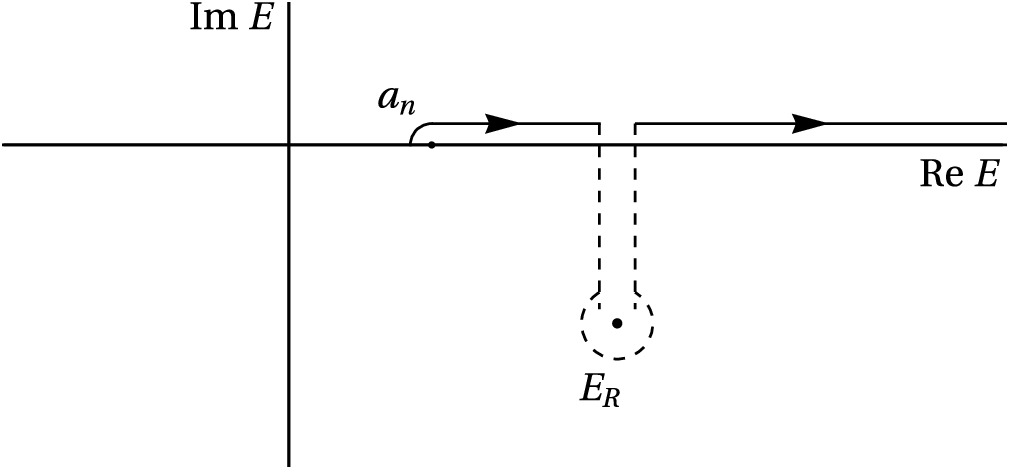
then, $ Z^{(i)}\equiv \sum_k Z^{(i)}_k $ is called the elementariness and $ X^{(i)}\equiv \sum_{m=1}^CX^{(i)}_m $ is called the compositeness for the bound state. When the solution $ E_i $ resides on the unphysical sheet, it is necessary to deform the integral contour to bypass the pole position in different integrals, as illustrated in Fig. 1. For resonance poles on the m-th sheet, the integral contour for the first m-th integral should be deformed accordingly, following the contour shown in Fig. 1. In such cases, the usual definition of the normalization may not be well-defined, as the integral contour for the pole and its conjugate pole are not consistent. Therefore, it becomes necessary to define the normalization through the inner product of the state and its conjugate state which corresponds to the conjugate pole. The resulting normalization is similar to Eq. (18) with $ E_i $ replaced by the pole position on the unphysical sheet and the integral contour suitably deformed. However, it is important to note that the probabilistic interpretation of each term in the sum will no longer hold, as the terms may not be real or positive for poles on the unphysical plane.

Figure 1.  The integral contour for the resonance solution.

Now we come to the case with degenerate threshold. If there are different continuum states with the same threshold $ a_n $, with degeneracy $ h_n $, we need to add another label κ to the continuum to denote the different continuum states sharing the same threshold, $ |\omega,n\kappa\rangle $. Thus all the indices in the equations labelling the continuum states would include the additional indices κ to label the degenerate states, for example, $ f_{in}(\omega) $, $ \alpha_{ni} $, $ \gamma_m $, $ \psi_{mn} $, $ \Psi_m $ become $ f_{i,n\kappa} $, $ \alpha_{n\kappa, i} $, $ \gamma_{m\kappa} $, $ \psi_{m\kappa,n\kappa'} $. There will be $ \mathfrak h=\sum_{n=1}^C h_n $ continuum states. The sum over the continuum states also needs to sum over the κ. The matrix $ \boldsymbol\gamma $ is defined as $ \gamma_{m\kappa,n\kappa'}(E)=\delta_{mn}\delta_{\kappa,\kappa'}\Theta(E-a_n) $. $ \mathbf f $ matrix becomes a $ D\times \mathfrak h $ matrix and $ \boldsymbol \eta $ is still a $ D\times D $ matrix. With all these changes, the previous discussion and equations can be smoothly used in this case.

In the previous case, we considered a scenario where a bare continuum state is only coupled to the bare discrete states but not to the other continuum states. However, when the direct interactions between continuum states become significant, it is more appropriate to include the corresponding term in the interaction Hamiltonian $ H_I $. Analytically solving the Hamiltonian with a general continuum-continuum interaction is generally not feasible. Therefore, in this section, we will focus on the case with a separable interaction, which still allows for an exactly solvable solution.

The Hamiltonian, including D discrete states and C continua with factorizable self-interacting contact terms, can be expressed as

In this case, the new coupling constants $ v_{mn} $ between two continuum states have been incorporated in the interaction terms, and $ v_{mn}=v_{nm}^* $ is satisfied to meet the Hermiticity requirement. The form-factor functions $ g_n(\omega) $ are involved in the interaction between two continuum states, and $ f_{jn}(\omega) $ represents the interaction vertex between the j-th discrete state and the n-th continuum state. We suppose $ f_{jn} $ matrix is of full rank, otherwise one can always find a decoupled state by linear combination of the discrete states or the continuum states. For the sake of simplicity, we first assume that the coupling constant matrix $ v_{mn} $ is non-degenerate and will come back to the degenerate $ v_{mn} $ case later.

Similar to the previous case, we are also going to solve the Hamiltonian eigenfunction $ H|\Psi(E)\rangle=E|\Psi(E)\rangle $. The eigenstate of the Hamiltonian with eigenvalue E can be be expanded in terms of the discrete states and the continuum states as

Inserting this ansatz into the eigenvalue equation and projecting to the discrete eigenstates or the continuum ones, one can find two sets of equations

where, two new integration functions $ A_j(E) $ and $ B_n(E) $ have been defined as

Since we have assumed that the continuum-continuum coupling constants $ v_{mn} $s are not degenerate, there are C independent $ B_n(E) $ functions. On the contrary, if $ v_{mn} $ matrix is degenerate, the only change is that there will be fewer $ g_n $ and $ B_n $ functions.

Similarly as discussed previously, if the eigenvalue $ E\in [a_l,a_{l+1}) $ for $ l< C $, there should be l continuum solutions $ |\Psi_m(E)\rangle $, $ m=1,2,\dots, l $ with the same eigenvalue E. As the interactions are gradually deactivated, it is required that these continuum solutions tends to well-defined states $ |E,m\rangle $. This ensures that in the absence of interactions, the continuum solutions can be uniquely determined as the continuum states $ |E,m\rangle $, thus eliminating any ambiguity in their characterization. This requirement guarantees a smooth transition from the interacting system to the non-interacting system.

Under these specific conditions, the l contiuum state solutions for $ a_l<E<a_{l+1} $ coincide with the first l states for $ E>a_C $. Consequently, it is sufficient to solve for the solutions when $ E>a_C $, and then the first l solutions can be obtained for the range $ E<a_l $. For each continuum state $ |\Psi_m(E)\rangle $ with $ E>a_C $, the corresponding coefficients are denoted as $ \alpha_{jm} $, $ \psi_{nm}(E,\omega) $, $ A_{jm} $, and $ B_{nm} $ as in eqs. (21), (22), and (23). Then, one could obtain

The procedure of solving the equation Eq. (26) is straightforward but intricate. The strategy is to apply the operations $ \sum_n\int_{a_n} d\omega f^*_{jn}(E)\times $ and $ \sum_n v^*_{nm'}\int d\omega g^*_{n}(\omega)\times $ on the left-hand side of Eq. (26), respectively. After this, we can derive the following expressions:

The matrix representation proves to be a valuable tool in simplifying the derivation process and achieving concise results. In this context, we introduce matrix $ \mathbf{Y} $ and $ \mathbf{F} $ with $ (C+D) \times C $ dimension, matrices $ \mathbf{V}^A $ and $ \mathbf{V}^B $, with dimensions $ D \times D $ and $ C \times C $ respectively, matrices $ \mathbf{V}^{AB} $ and $ \mathbf{V}^{BA} $, having dimensions $ D \times C $ and $ C \times D $ respectively, and finally, a $ (C+D) \times (C+D) $ matrix $ \mathbf{M} $ encompassing $ \mathbf{V}^A $, $ \mathbf{V}^B $, $ \mathbf{V}^{AB} $ and $ \mathbf{V}^{BA} $ as follows

Similar to the coefficients α and ψ, we have omitted the superscript $ \pm $ in the notations of the matrices $ \mathbf Y $, $ \mathbf V $, and $ \mathbf M $, which can be inferred from the surrounding contexts. With these matrices, the two equations (27) and (28) above can be expressed in matrix form

or in component form

Before further proceeding, let us look at some properties of these matrices. From the relation $ v^*_{mn}=v_{nm} $, we can observe the following symmetric properties:

In the case where $ v_{mn} $, $ f_{jm}(\omega) $ and $ g_n(\omega) $ are real for real ω, these function matrices possess real analyticity property. As a result, they can be analytically continued to the entire complex E plane and satisfy the Schwartz reflection property. Moreover, the analytically continued function matrices can relate the $ +i0 $ and $ -i0 $ counterparts, representing the limits on the upper and lower edges along the real axis above the threshold. In the cases that $ v_{mn} $, $ f_{jm}(\omega) $ and $ g_n(\omega) $ are complex, the function matrices will no longer be real analytic, but the determinant of the matrix $ \mathbf M $, denoted as $ \det \mathbf M $, remains real analytic. Thus the analytically continued determinant exhibits the Schwartz reflection symmetry, $ \det \mathbf M(z)=\det \mathbf M^{*}(z^*) $.

In general, $ \det \mathbf M $ is nonzero for general real E values above the lowest threshold, otherwise if $ \det \mathbf M=0 $ for all real E, $ v_{mn} $ matrix would be degenerate and there would be a state decouples in continuum-continuum interaction, which is not our assumption at present. As a result, $ \mathbf M $ possesses an inverse. and $ \mathbf Y $ can be obtained by $ \mathbf Y= \mathbf M^{-1}\cdot \mathbf F $. Then, by inserting $ A_{jm}(E) $ or $ \alpha_{jm}(E) $ and $ B_{nm} $ into Eq. (26), one obtains the coefficients $ \psi^\pm_{nm} $, and the continuum eigenstates are solved to be

for $ E>a_m $. Upon comparison with Eq. (12), this solution is different only in the last term, stemming from the presence of separable potential. Importantly, it can be confirmed that the solution retains the previous normalization condition, $ \langle \Psi^\pm_m(E)|\Psi^\pm_n(E')\rangle=\delta(E-E')\delta_{mn} $. This normalization condition guarantees the orthogonality of the wave functions, ensuring their compatibility and consistency within the framework of the problem.

The S-matrix can be obtained as

or

in a simplified matrix form. For a more thorough derivation of the normalization and meticulous calculation of the S-matrix, please refer to the Appendix A, where we provide a detailed presentation of the calculations, offering a comprehensive and in-depth derivation of the normalization condition and the S-matrix.

Subsequently, our attention turns towards the derivation of discrete eigenstates. The eigenvalues for the discrete states does not coincide with the spectrum of the continuum states. Thus, using the condition $ E\notin [a_i,\infty) $ for $ i=1,\dots, C $, Eq.(23) one can solve Eq.(23) and obtain

By multiplying Eq. (39) with $ f^*_{jn}(\omega) $ and $ v^*_{nm}g_n^*(\omega) $ separately, and subsequently summing over n and integrating w.r.t. the variable ω, we arrive at the following expressions:

The expressions obtained in these two equations deviate from (27) and (28) by the absence of the first terms on the right hand side. Analogous to the definition in Eq. (30), we can introduce the matrices $ \mathbf V^A $, $ \mathbf V^{AB} $, $ \mathbf V^{BA} $, $ \mathbf V^B $, and $ \mathbf M $ as the analytic continuation of the matrices in Eq. (30) and

Then Eqs.(40) and (41) can be expressed as

To obtain nonzero solutions for the vector $ \mathbf X $, it is essential to satisfy the condition that the determinant of $ \mathbf M $ is equal to zero, i.e., $ \det \mathbf M(E)=0 $. By analytically continuing this equations to different Riemann sheets and solving it on each sheet, we can determine the generalized discrete eigenvalues.

Once the generalized eigenvalues are determined, the vector $ \mathbf X $ can be solved for each eigenvalue. Substituting the solutions for $ \alpha_j $ and $ B_n $ into Eq. (39), we obtain the discrete solution from Eq. (21) for each generalized energy eigenvalue,

where the superscript $ (i) $ denotes the i-th discrete solution. The solution for $ \mathbf X $ is only determined up to a normalization. On the first Riemann sheet, the zeros of the $ \det \mathbf M $ can only be located on the real axis below $ a_1 $ due to the hermicity of the Hamiltonian. These zeros correspond to the discrete eigenvalues $ E_b $. It is possible for the associated states to have a finite norm, and we can impose the normalization condition on the coefficients to ensure

Within the framework described earlier, each term in the summation can be interpreted as the probability of finding the corresponding bare state within the bound state. However, there could also be complex energy solutions present on different unphysical sheets. As the determinant of $ \mathbf M $ is a real analytic function, these complex eigenvalue solutions appear as complex conjugate pairs.

As already mentioned, there exist $ 2^C $ distinct Riemann sheets. However, for our specific purposes, we focus solely on solutions $ E_R $ that reside on the lower half Riemann sheet closest to the physical sheet. These solutions have a significant impact on the physical S-matrix elements. Since $ E_R $ lies on a nearby unphysical sheet, the evaluation of the matrix value of $ \mathbf M $ at this point requires deforming the integral contours to the corresponding sheet around $ E_R $ defined in the matrix $ \mathbf V $ and $ \mathbf M $ in Eq. (30) as illustrated in Fig. 1 [5]. Also in the state solution Eq.(42), the integral contours are also deformed similarly. The normalization requirement of these states may resemble Eq.(43), but with $ E_b $ replaced by $ E_R $, and the integral contour adjusted accordingly following the deformation depicted in Fig. 1. However, it is important to note that there is no probabilistic explanations for each terms in the sum, as they may not be real. Additionally, there can also be real solutions below the lowest threshold $ a_1 $ on unphysical sheets, which correspond to virtual states. Similar to the resonant states, the corresponding integral contours should be deformed in Eq. (42) and in Eq. (30) for these states.

In the case where the coupling constant matrix $ v_{mn} $ is degenerate, certain continuum states may decouple from the contact interaction. This allow us to choose a suitable set of continuum basis states in which the decoupled states do not appear in the contact interaction terms. A more general hamiltonian can be expressed as

where r is the rank of the continuum-continuum coupling constant matrix and $ v_{mn} $, $ m,n=1,\cdots,r $ is a non-degerate matrix. Notice that in general, though we are discussing the case for degererate case where $ r<C $, this general interaction even applies for the cases when $ r>C $ which may correspond to the case we will discuss in the next section. Since v is a hermitian matrix, it can always be diagonalized and be chosen as $ v_{mn}=\lambda_m\delta_{mn} $, for $ m,n=1,\cdots,r $. When $ g_{mm'}\propto \delta_{mm'} $, it reduces to the original case (20). The solution to the engenvalue problem for this Hamiltonian is straightforward as before. The difference of the results from the nondegerate case is roughly to change definition of $ B_n $ in Eq. (24) by $ B_n= \sum_{l=1}^C \int g_{nl}\psi_l $ ($ n=1,\cdots,r $) and replace the factor $ v_{nm} g_n $ to $ \sum_{l=1}^r v_{lm}g_{ln} $ in each equation. For different continuum solution $ B_n $ would need another index m to denote the corresponding continuum solution, i.e. $ B_{nm} $, $ (n=1,\cdots,r; m=1,\cdots,C) $. Notice that the range of the first subindex of $ g_{ln} $ and $ B_{nm} $ is from $ 1 $ to r and the second one from $ 1 $ to C. Thus the sum of the first subindex of $ g_{ln} $ of $ B_{nm} $ need to be from $ 1 $ to r.

A special case is when $ r=1 $ and we can set $ v_{11}=1 $ and $ g_{1n}= v_n g_{n}(E)\equiv (\mathbf g)_n $ where $ v_n $ is a constant and $ g_n(E) $ is a coupling function. Then the we can rename $ B_{1m} $ to $ B_m^\pm(E)\equiv B^\pm _{1m}=\sum_{n=1}^C v_n \int d\omega g_n(E)\psi^\pm_{nm}(E) $. The $ \mathbf M $ matrix in Eq. (30) can be represented as

For the continuum eigenstate solutions, $ \alpha_{jm} $ and $ B_m $ are solved as

where we have defined the vector $ (\mathbf f_m)_i=f_{im} $, $ i=1,\cdots,D $. Then the S-matrix can be obtained as

With the S matrix, the observable scattering cross section can be obtained to compare with the experiments.

In the spirit of effective field theory, a discrete state $ j_0 $ become decoupled when its mass $ M_{j_0} $ greatly exceeds the system's characteristic energy scale. This fundamental principle was exemplified in Weinberg's seminal work [29], where two equivalent formulations were constructed: the full theory contains the discrete state explicitly in the free Hamiltonian, while the reduced theory eliminates the discrete state by introducing a specific potential renormalization. Weinberg demonstrated their equivalence when $ M_{j_0}\to \infty $, provided the potentials satisfy the matching conditions that encode the decoupling dynamics. In our present scenario, we can also construct a low energy effective Hamiltonian without this discrete state and include an effective contact interaction of the continuum states after integrate out the intermediate discrete state in s channel. The corresponding interaction term can be expressed using separable contact effective interaction terms as

This interaction is similar to the previous special case with $ r=1 $ by replacing $ v_{11}\to v_{j_0j_0}=-1 $, and $ g_{1n}\to g_{j_0 n}=\dfrac{f_{j_0 n}}{\sqrt{M_j}} $, and the matrix elements $ v_{j_0,n}=0 $ and $ g_{mm'}=g_m\delta_{mm'} $. It effective adds one extra rank to the original $ v_{mn} $ matrix. To solve this eigenvalue problem, using Eq. (30) and previous discussion below (44), there will be a row and colomn in the $ \mathbf V^B $ from the (54), with

For $ \mathbf V^{AB} $, there will be corresponding matrix elements

and similar for $ \mathbf V^{BA} $. For $ \mathbf F $, there is an element $ \mathbf F_{j_0,n}=-f^*_{j_0 n}/\sqrt{M_{j_0}} $. Alternatively, we can start from the original Hamiltonian with the discrete state and taking the large $ M_{j_0} $ limit. From Eq. (30), taking $ M_{j_0} $ much larger than E in $ \mathbf V^{A}_{j_0j_0} $ is to factorize the $ M_{j_0} $ and take $ E/M_{j_0}\to0 $, i.e. making the replacement $ \mathbf V^{A}_{j_0j_0}\to M_{j_0}(-1- \dfrac 1 {M_{j_0}} \sum_{n=1}^C\int_{a_n}d\omega\dfrac{f_{j_0n}(\omega)f^*_{j_0n}(\omega)}{E-\omega\pm i0}) $. Similarly, after factorizing out $ M_{j_0} $ from $ \mathbf V^A_{j_0 j_0} $, and $ \sqrt{M_{j_0}} $ from $ \mathbf V^A_{ij_0} $, $ \mathbf V^A_{j_0i} $, $ \mathbf V^{AB}_{j_0m} $, $ \mathbf V^{BA}_{mj_0} $, these matrix elements are of the same form as the corresponding matrix elements in $ \mathbf V^{AB} $, $ \mathbf V^{BA} $, $ \mathbf V^B $ in (56) and (55) as if one is directly solving the decoupled Hamiltonian as constructed above (54). One can then find out that the S matrices obtained by the two approaches are the same.

In scenarios where the interaction potential can be reasonably approximated as separable potentials, wherein the potential can be expressed as the product of two components associated with the ingoing and outgoing states, respectively, the problem can be effectively addressed and hold practical significance. Now the problem is how to approximate a potential using the separable potentials. Before addressing this problem, let us review how a general contact interaction can arise in the elastic and nonelastic scattering.

As discussed in the previous section, the Hamiltonian of a most general model with multiple discrete states and continuum states and their interactions can be expressed as

In the context of nonrelativistic scattering, i.e. when the in-state and out-state are composed of the same two-particle content, in the angular momentum representation, these continuum states can be expressed as $ |\omega,n\rangle=\sqrt{\mu p}|p,JM;lS\rangle $, where $ J,M,l,S $ are the quantum numbers for total angular mentum, magnetic angular momentum, relative orbital angular momentum, and total spin, respectively, and are collectedly denoted using n and $ a_n $ are the threshold. Here, p represents the radial momentum, μ is the reduced mass and $ \omega=\dfrac{p^2}{2\mu}+a_n $ represents the total energy. The normalization of the continuum states is chosen such that the inner product between two continuum states is given by $ \langle \omega',n'|\omega,n\rangle= \delta_{n'n}\delta(\omega-\omega') $. The momentum space potential $ V_{mn}(\omega',\omega) $ can be derived from the coordinate space potential $ V( {\mathbf r}) $. For simplicity, we consider only the rotational invariant potential. The potential function $ V_{mn}(\omega',\omega) $ arises from the matrix elements $ V_{n'n}(\omega',\omega)\equiv\langle \omega',n'|V|\omega, n\rangle= \sqrt{\mu' p'}\sqrt{\mu p}\,\langle p'JMl'S'|V|pJMlS\rangle $. The simplest example is when the in-states and out-states are composed of the same spinless particles, i.e. elastic scattering. If we know the coordinate-space potential $ V(r) $, then the momentum-space potential $ V(k',k) $ can be expressed in terms of the coordinate-space potential $ V(r) $ as follows:

where the $ {\hat j}(z) $ represents the Riccati-Bessel function.

In the cases where the in-states and out-states can have different particle compositions, we can generalize the potential $ V(\omega',\omega) $ accordingly. In addition to the angular momentum quantum numbers, the labels n and $ n' $ can also denote the different particle compositions $ |\omega,n\rangle $. If the potential in coordinate space, $ V( {\mathbf r}', {\mathbf r}) $, in the center-of-mass system, is invariant under rotation, it can be expressed as a function of $ {\mathbf r}^2, {\mathbf r}'^2 $ and $ {\mathbf r}\cdot {\mathbf r}' $. Here, $ {\mathbf r} $ and $ {\mathbf r}' $ represent the position of the in-state and out-state relative coordinates,respectively. In the case of spinless particle system, the matrix elements for in-states and out-states can be expressed as follows:

The Wigner-Ekart theorem has been employed to account for the spherical symmetry of the potential $ V( {\mathbf r}', {\mathbf r}) $. When the in-state and out-state can have spins, the total angular momentum are conserved but the orbital angular momentum could be different. We can include the different orbital angular momentum and total spin quantum numbers $ lS $ and $ l'S' $ into n and $ n' $ to label different in-states and out-states,

where $ C^{JM}_{lmSm_s} $ is the Clebsch-Gordon coefficients. To make further progress, we also suppose that the potential is square integrable for both $ \omega' $ and ω, and the same for the interaction vertex between the discrete states and the continuum states $ f_{jn}(\omega) $, that is

There are no exact solutions for Hamiltonian for general potentals $ V_{mn}(\omega',\omega) $. However, it is well-known that such a potential can be expanded using a sum of separable potentials [30]. For continuum states $ |\omega,m\rangle $, we can choose a set of complete basis functions $ \tilde g_{m\rho}(\omega) $, with $ \int_{a_m} d\omega \tilde g^*_{m\rho}(\omega)\tilde g_{m\delta}(\omega)=\delta_{\rho\delta} $ and $ \sum_\delta \tilde g_{m\delta}(\omega')\tilde g_{m\delta}(\omega)= \delta(\omega'-\omega) $. The basis sets for different continuum states, i.e. for different m and n, do not need to be the same. The potential $ V_{mn}(\omega',\omega) $ can then be expanded as

In the following we will use the Greek letter ρ, δ to label the basis, and repeated Greek letters are summed over without explicit sum symbol and the sum symbol for the Latin letters would still be left explicit. The coefficient matrix composed of $ v_{mn,\rho\delta} $ is hermitian $ v_{mn,\rho\delta}=v^*_{nm,\delta\rho} $ and is supposed to be non-degenerate. In general, there are infinite number of bases, the sum of δ and ρ is up to infinity. Since the expansion coefficients $ v_{mn,\rho\delta} $ are small at large enough order, one can make an approximation and truncate the series to a finite order N, i.e. $ v_{mn,\rho\delta}=0 $ for $ \rho,\delta>N $. Then, the general Hamiltonian for multiple continuum states and discrete states can be recast as

One can take $ m\rho $ and $ n\delta $ as the row and column indices and diagonalize the matrix $ v_{mn,\rho\delta} $. Then, the problem reduces to the similar case in the last part of the last section when the degenerate $ v_{mn} $ is discussed. Here the rank of $ v_{mn,\rho\delta} $ is greater than C just as we mentioned in last section. Alternatively, we can also directly solve the problem as before in the following. The general eigenstate for this eigenvalue problem can be expanded using the bare discrete states and the bare continuum states

Similar to previous sections, for $ |\Psi_m\rangle $, the corresponding $ \alpha_i $ and $ \psi_n $ will have another index m, i.e. $ \alpha_{im} $ and $ \psi_{nm} $.

With the same procedures as the previous section, the approximate properly normalized continuum states can be solved as

where $ \alpha^\pm_{im}(E) $ and $ \psi^\pm_{n'm\rho}(E)\equiv\int_{a_n}^\infty \psi_{n'm}(\omega)\tilde g_{n\rho}(\omega) $ can be solved as in Eq.(B11). The S-matrix can then be obtained,

where the matrix $ \tilde{\mathbf M}^+ $ with dimension $ (D+NC)\times (D+NC) $ and vector $ \tilde {\mathbf F}_m $ with dimension $ (D+NC) $ are defined in Eq.(B7). The detailed calculation is left to appendix B. The discrete eigenvalues can be obtained by solving Eq. $ \det \tilde {\mathbf M}(E)=0 $. The discrete state corresponding to eigenvalue $ E_i $ can be expressed as

where the integral contour needs to be deformed for $ E_i $ on unphysical sheets as before.

It is worthful to mention that though we are choosing $ g_{m\delta} $ as orthogonal function sets, we do not use this orghogonal property in solving the problem. Thus, as long as we can approximate the Hamiltonian using the separable interaction like in (58) without orthogonal conditions for $ g_{m\delta} $ functions, the solution applies.

Next, we could go further and also expand the interaction function $ f_{jm}(\omega) $ using the same set of basis $ \tilde g_{m\delta}(\omega) $ as in the corresponding contact interaction involving the continuum state $ |\omega,m\rangle $,

and also make an approximation by truncating the series to the N-th order the same as in the contact terms, that is, $ f_{jm\delta}=0 $ for $ \delta>N $. This may reduce the dimension of the matrix $ \tilde{\mathbf M} $ and may also simplify the numerical calculation. Then, the general Hamiltonian for multiple continuum states and discrete states can be recast as

This case is more like the cases discussed in [10, 26], where the same form factor comes with the continuum both in the discrete-continuum and continuum-continuum interaction. Using the eigenstate ansatz

one can proceed solving the eigenvalue problem similarily to the previous section, of which the details will be left to appendix C. The properly normalized continuum state can be solved and expressed as

where the $ \alpha^\pm_{im} $ and $ \psi^\pm_{nm\rho} $ can be solved from Eq.(C9). The S-matrix can be obtained

where the $ NC\times NC $ matrix $ \tilde {\mathbf W}^+ $ and $ NC $ dimensional vector $ \tilde {\mathbf F}_m $ are defined in Eq. (C8) and Eq. (C7). Similar to previous section, the generalized energy eigenvalues for the discrete state can be obtained from the $ \det \tilde {\mathbf M}(E)=0 $, and for each eigenvalue $ E_i $, $ \psi_{n\rho}^{(i)} $ can be solved from $ \tilde {\mathbf M}\cdot \tilde {\mathbf Y}=0 $, where the matrix $ \tilde {\mathbf M} $ and $ \tilde {\mathbf Y} $ are defined in Eq. (C6) and Eq. (C7). Then we have the discrete eigenstates,

with integral contour deformed for resonances and virtual states as before.

In the case when there are contact interactions involved, we can explore the effect of introducing small couplings on the mass of the discrete states in a general manner. Analyzing pole trajectories as couplings vary offers valuable insights into particle properties. This type of analysis proves useful in elucidating the origin of certain states observed in the experiments utilizing Friedrichs-like models or similar formulas derived from the dispersive models. Notably, refs. [21, 31−34] demonstrate how pole trajectories of various states provide valuable clues regarding the possible nature of these particles. Moreover, such analyses may also provide qualitative guidance in understanding the interaction properties from the spectrum. To illustrate this, we focus on the exponential form factor, a frequently employed form factor in the literature. Using this form factor as an example, we discuss the properties of the bound states while varying the couplings. For simplicity, we consider a two-channel case where the threshold for the two continuum states are denoted as $ a_1 $ and $ a_2 $ with $ a_1<a_2 $.

The basic consideration is as follows: At the leading order, where the interactions are absent, the discrete state is determined by the condition $ E-\mu=0 $, with the bare mass being the solution. When a small coupling constant λ is turned on, we must consider an equation of the form $ E-\mu+\lambda \chi(E)=0 $ ($ \lambda>0 $), where $ \chi(E) $ is real and small in the vicinity of $ E=\mu $. The next-to-leading-order solution can be expressed as $ E=\mu-\lambda \chi(\mu) +O(\lambda^2) $. The sign of $ \chi(\mu) $ allow us to determine the tendency of the solution's behavior. If we know that $ \chi(E) $ is a monotonic function, either positive definite or negative definite, we can determine the direction in which the solution will shift as λ increases continuously. For example, if $ \chi(E) $ is a positive decreasing function, it is evident that the solution will move downward as λ becomes increasingly positive. More generally, when we replace the left-hand side of the leading-order equation $ E-\mu=0 $ with another increasing function, i.e. $ \zeta(E)=0 $, the addition of another positive increasing function will cause the zero point to shift to the left. See Fig. 2 for an illustration.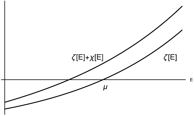

Figure 2.  A monotonic increasing function $ \zeta(E) $ which satisfies $ \zeta(\mu)=0 $. The solution for $ \zeta(E)+\chi(E)=0 $ is smaller than μ if $ \chi(E) $ is a monotonic increasing positive function.

We also need to examine the behavior of the dispersion integral defined as $ G(E)=\int_a^\infty d\omega \dfrac{ |f(\omega)|^2}{E-\omega +i0} $. When $ E<a $, the integral behaves as a purely negative decreasing function. For $ E>a $, the imaginary part is $ -\pi |f(E)|^2 $, which is purely negative in this region. The real part corresponds to the principal value integral in $ G(E) $. Near the threshold, the real part is negative and increasing with E, passing through zero point $ \hat E $ and reaching a positive maximum, and then decreases back towards zero as E approaches infinity. See Fig. 3 for an example. Typically, the integrand includes a phase space factor $ \rho(E)\propto \sqrt{E-a_1} $ which suppresses the integrand near the threshold a, which causes a higher value of $ \hat E $. See Fig. 3 for the case with $ |f(\omega)|^2=\sqrt{\omega-a_1} e^{-E/\Lambda} $. We observe that $ \mathrm{Re}G(E) $ becomes positive only when E approaches Λ, which characterizes the inverse of the interaction range. If the energy range of interest is significantly smaller than Λ, then $ \mathrm{Re} G(E) $ remains negative. We will primarily focus on this region below.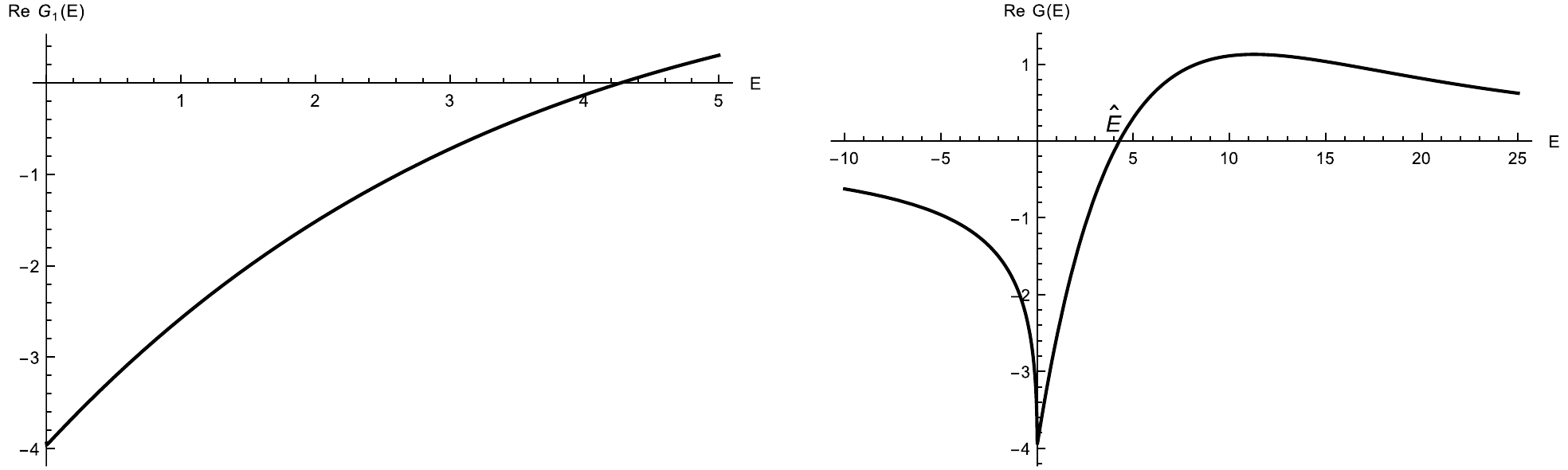

Figure 3.  The general behavior of the real part of $ G(E)=\int_{a}^\infty d\omega \frac{|f(\omega)|^2}{E-\omega+i\epsilon} $ function, using $ |f(\omega)|^2=\sqrt{\omega-a} e^{-\omega/\Lambda} $, with $ \Lambda=5 $, $ a=0 $. If the interested energy region is much smaller than Λ, then $ \mathrm {Re} G(E)<0 $.

With this preparation, we can explore some interesting and instructive simple cases that are relevant to the phenomenological analysis of the spectrum.

First, we consider the cases with only continuum states.

1. In the presence of a single continuum and self interaction $ v_{11} $, if $ v_{11} $ is sufficiently negative (i.e. attractive), a bound state will emerge at $ E_0<a_1 $.

This is the simplest case. The $ \mathbf M $ matrix reduces to a function,

where $ G_1=\int_{a_1}^\infty d\omega \dfrac{|g_1(\omega)|^2}{E-\omega+i\epsilon} $ and $ a_1 $ is the threshold. Since $ G_1(E) $ is negative and continuously decreasing for $ E<a_1 $ with $ \lim_{E\to -\infty} G_1(E)=0 $, as shown in Fig. (3), for $ M_{11} $ to have a zero point at $ E_0<a_1 $, the coupling $ v_{11} $ must satisfy the condition $ v_{11}< 1/G_1(a_1) $.

2. With a second continuum state included, we can examine the coupled-channel effect on the dynamical bound state of the lower channel discussed in previous case when $ v_{11}<0 $.

The $ \mathbf M $ matrix becomes

where $ a_1 $ and $ a_2 $ are the thresholds for the two channels with $ a_1<a_2 $. The determinant can be calculated to be

It is worth mentioning that since $ v_{12} $ appears only in $ \det \mathbf v $ in the form of $ |v_{12}|^2 $, the phase or sign of $ v_{12} $ is irrelavent to this result in this context.

There are four cases to consider progressively. In each case we will first present the result and then provide the reasoning behind it.

(a) When $ v_{12}\neq 0 $ and $ v_{22}=0 $, the coupled channel effect will play a role of attractive interaction, causing the bound state to shift from $ E_0 $ to a deeper energy level $ E_{0b} $, i.e. $ E_{0b}<E_0 $.

This can be demonstrated by directly calculating the determinant of $ \mathbf M $, yielding

At $ E<a_1 $, the last term $ -|v_{12}|^2G_1(E)G_2(E) $ in the bracket is negative and decreasing, while the term $ -v_{11}G_1(E) $ is also negative and decreasing. Following similar reasoning as illustrated in Fig. 2, E must be much smaller in order to have a zero point of $ \det\mathbf M $, denoted as $ E_{0b} $. This discussion does not rely on the smallness of the coupling, and therefore it is also valid for strong interaction.

(b) When a sufficiently small $ v_{22} $ is then turned on, the result depends on the sign of $ v_{22} $. A negative $ v_{22} $ causes the bound state to shift to a deeper energy level, while a positive $ v_{22} $ results in a shallower bound state.

The contribution from $ v_{22} $ to the $ \det \bf M $ at the zero point $ E_{0b} $ can be expressed as

When the $ v_{22} $ is negative, indicating a more attractive interaction, this term contributes positively to $ \det \mathbf M $ for $ E<a_1 $, thereby negatively affecting the terms in the bracket of (69). This results in the bound state shifting deeper from $ E_{0b} $, moving away from the threshold. Conversely, when $ v_{22} $ is positive, the bound state becomes shallower, moving upward from $ E_{0b} $. Therefore, when both $ v_{12} $ and a positive $ v_{22} $ are present, the direction of the bound state's movement from $ E_0 $ depends on the competition between the effects of $ v_{22} $ and $ v_{12} $.

(c) For large $ |v_{22}| $, when $ v_{22}>0 $, we can conclude that the bound state will be located to the left of $ E_0 $ but to the right of $ E_{0b} $.

This can be understood by expressing $ \det \mathbf M $ as follows:

and by considering the positivity of $ -v_{22}G_2(E) $ in the last term in the bracket for $ E<a_1 $. As $ v_{22} $ increases, the absolute value of the last term in the bracket deceases. Thus, when positive $ v_{22} $ is turned on from $ 0 $ to $ \infty $, the bound state moves from $ E_b $ to $ E_0 $.

(d) When negative $ v_{22} $ is introduced, starting from zero and becomes increasingly negative, the bound state will shift deeper from $ E_{0b} $ to $ -\infty $.

This occurs because, for fixed E, the term $ 1-v_{22}G_2(E) $ in the denominator of the last term in the bracket approaches zero, leading to a divergence of that term. To cancel the first two finite terms, E must become increasingly negative so that $ |G_2(E)| $ decreases sufficiently, allowing the last term to remain finite and effectively cancel the first two terms in the bracket. Consequently, this will cause the bound state to shift deeper from $ E_{0b} $ to $ -\infty $.

3. Similar to previous case, when there is only an attractive interaction in the second channel, i.e. $ v_{22}<0 $ with $ v_{11}=v_{12}=0 $, a dynamically generated bound state ($ E_b $) can exist below $ a_2 $ and is assumed to be above $ a_1 $, satisfying the condition $ 1/G_{22}(a_1)<v_{22}<1/G_{22}(a_2) $. We can then examine the effect of turning on the first channel on the bound state spectrum of the second channel. There are two cases to consider.

(a) When a small $ v_{12} $ is introduced while keeping $ v_{11}=0 $, the bound state will transit to the second sheet. Whether the mass of the state increases or decreases depends on the sign of $ \mathrm{Re} G_1(E_b) $. A negative $ \mathrm{Re} G_1(E_b) $ will cause the mass of the state tend to decrease, while a positive $ \mathrm{Re} G_1(E_b) $ will lead to an increase in the mass.

In this case, we have

Consider solving $ \det M=0 $ in the powers of $ v_{12} $ using iteration. Since $ E_b>a_1 $, the $ G_1(E) $ factor in the last term contributes an imaginary term of $ -\pi i |g_1(E)|^2 $. Combining this with the other factors yields a negative imaginary part on the order of $ |v_{12}|^2 $ in the bracket. For $ \det M=0 $ to hold, the state corresponding to $ E_b $ must move into the complex plane, allowing the term $ -v_{22}G_2(E) $ to generate a negative imaginary part of order $ v^2_{12} $ to cancel the imaginary part of the last term in the bracket. Thus, E must have a negative imaginary part, and with the $ +i\epsilon $ in the definition of $ G_i(E) $, the pole moves continuously to the second Riemann sheet. This is consistent with the common knowledge that the resonance poles can not reside on the physical sheet. Whether the mass of the pole is increasing or decreasing depends on the the sign of the leading real part of the last term, which is determined by examining $ \mathrm{Re} G_1(E_b)=P.V.\int_{a_1}^\infty d\omega \dfrac{|g_1(\omega)|^2}{E_b-\omega} $. If this value is negative(positive) the mass will decrease(increase). This is due to $ G_2(E) $ being negative and decreasing for $ E<a_2 $, leading to a negative (positive) contribution from the real part of the last term in the bracket. In the example illustrated in Fig. 3, when Λ is much larger than $ a_2 $ where $ \mathrm{Re} G_1(E) $ is negative and monotonically increasing near $ E_b $, turning on the $ v_{12} $ will cause the mass of the dynamically generated state (from $ E_b $) in the second channel to decrease.

(b) When a small $ |v_{11}| $ is also turned on, as long as $ |v_{11}| $ is small enough, the result will be the same as previous case.

Similar to previous case, $ \det \mathbf M $ can be expressed as

Compared to (71), there is an extra factor $ 1/(1- v_{11}G_1) $ in the $ |v_{12}|^2 $ term. The difference is of order $ O(v_{11}|v_{12}|^2) $, and therefore, for sufficiently small $ |v_{11}| $, the result would be the same as in the previous case.

4. There could also be a bound state generated from pure $ v_{12} $ interaction with no self-interaction, i.e. $ v_{11}=v_{22}=0 $, regardless of the sign of $ v_{12} $. In this case, $ v_{12} $ acts as an attractive interaction.

If $ v_{11}=v_{22}=0 $, $ \det \mathbf M=-|v_{12}|^2(1-|v_{12}|^2G_1(E)G_2(E)) $. Since both $ G_1(E) $ and $ G_2(E) $ are negative and decreasing for E below the first threshold, there can be a solution to $ \det \mathbf M=0 $ when $ |v_{12}|^2 $ is sufficiently large, specifically when $ |v_{12}|^2>1/(G_1(a_1)G_2(a_1))) $. When $ |v_{12}|^2 $ decreases, the bound state will go up through the threshold to the second Riemann sheet, becoming a virtual state or a resonance. Thus, activating only $ v_{12} $ is equivalent to enhance the attractive interaction when there are only two continuum states.

Next, we add a discrete state of bare mass μ with coupling vertex functions to the two continua, $ f_1(\omega) $ and $ f_2(\omega) $. Now $ \mathbf M $ matrix becomes

where $\mathcal F_{n}=\int_{a_n}d\omega\dfrac {f_{n}(\omega)f_{n}^*(\omega)}{E-\omega+ i0}$, $\mathcal F^g_{n}=\int_{a_n}d\omega\dfrac {f^*_{n}(\omega)g_{n}(\omega)}{E-\omega+ i0} $, $ \mathcal F^{g{\text ‡}}_{n}=\int_{a_n}d\omega\dfrac {f_{n}(\omega)g^*_{n}(\omega)}{E-\omega+ i0} $.

We look at three different cases.

1. One bare discrete state coupled with two continuum states with $ v_{ij}=0 $.

When there is only the interaction between the discrete state and the continuum states, i.e. $ v_{11}=0, v_{12}=0, v_{22}=0 $, we need only to look at

By default, we will suppose $ \mu\ll \Lambda $, and $ \mathrm {Re} \mathcal F_1(\mu)<0 $ similar to Fig. 3.

(a) When $ \mu<a_1 $, since $ \mathcal F_1(E) $ and $ \mathcal F_2(E) $ for $ E<a_1 $ are negative and decreasing, the solution, denoted as $ E_\mu $, will be less than μ. This indicates that when the discrete state lies below both continuum states, turning on the interaction between the discrete state and the continuum states causes the discrete state move deeper below the thresholds.

(b) For $ a_1<\mu<a_2 $, when the sufficiently weak interactions $ f_1 $ and $ f_2 $ are gradually turned on, the discrete state would move to the second sheet and the mass will go down.

In this case, only $ \mathcal F_{1,2} $ contributions near μ are significant to the shift of the zero point, as observed in the iteration solution. With $ \mathcal F_2(\mu)<0 $, and assuming $ \mathrm{Re} \mathcal F_1(\mu) <0 $ (as seen in the case of exponential form factor with $ \mu\ll \Lambda $), a weak interaction between the discrete state and the two continua will also lead to a decrease in the mass of the discrete state. Since $ \mathcal F_1(\mu) $ has a negative imaginary part, the energy of the discrete state solution and $ -\mathcal F_2(E) $ will develop negative imaginary parts to cancel it. As a result, the discrete state will move continuously to the complex plane of the second Riemann sheet.

(c) When $ \mu>a_2 $, similar to the previous case, the discrete state will go to the third Riemann sheet and the mass will decrease.

The discussion is similar to the previous item. When $ \mu\ll \Lambda $, we find that $ \mathrm {Re}(\mathcal F_{1,2}(\mu)) <0 $, and these terms act as attractive interactions, driving the mass of the discrete state downward. The negative imaginary parts of $ \mathcal F_{1,2}(\mu) $ result in the solution moving down to the third sheet of the Riemann surface.

This may provide an understanding of why most of the open-flavor effects tend to cause the mass of the $ c\bar c $ state smaller [35]: The Λ in the corresponding system is large enough or the interaction range is so small such that $ \mathrm {Re}(\mathcal F_{1,2}(\mu)) <0 $.

2. One bare discrete state coupled with two continuum states with $ v_{11}\neq 0 $.

Now, proceeding from previous case, we gradually turn on $ v_{11}\neq 0 $ and leave $ v_{12}=v_{22}=0 $. Then we need to examine the zero point of the determinant of the first $ 2\times 2 $ submatrix, denoted as $ \mathbf M_{12} $

(a) We first consider $ E_\mu<a_1 $. We continue to use $ E_\mu $ to denote the solution to $ M_{11}=(E-\mu)-\mathcal F_1-\mathcal F_2=0 $, meaning that the discrete state is renormalized from the bare mass μ to $ E_\mu $ by turning on $ f_1 $ and $ f_2 $. There may also be another bound state dynamically generated by the continuum-continuum interaction $ v_{11} $, denoted by $ E_0 $, which arises from the solution to $ 1-v_{11}G_1(E)=0 $ when $ f_1=0 $, as discussed in case 2. We would examine the effect of turning on $ v_{11} $ on the bound state $ E_\mu $ and then the effect of turning on $ f_{1,2} $ on the bound state $ E_0 $.

● The simplest case is when $ v_{11}>0 $, no bound state is developed by pure continuum-continuum interaction. Turning on $ v_{11} $ will cause the bound state move upward toward the threshold from $ E_\mu $.

This occurs because at $ E=E_\mu $, the last term in (75) becomes $ |v_{11}\mathcal F^g_{1}(E_\mu)|^2>0 $ and $ (v_{11}(1-v_{11}G_1(E_\mu)))>0 $, while $ \mathcal F_{1,2}(E_\mu) $ are negative. Thus, turning on $ v_{11} $ has the opposite effect of $ \mathcal F_{1,2} $ on the discrete state. So, the state moves upward from the previous solution $ E_\mu $ toward the threshold.

● If $ v_{11}<0 $, the bound state would always move down from $ E_\mu $.

We first consider the case when $ |v_{11}| $ is sufficiently small, such that $ |v_{11}\mathcal F^g_{1}(E_\mu)|^2/(v_{11}(1-v_{11}G_1(E_\mu)))<0 $. This condition will cause the discrete states corresponding to $ E_\mu $ to move downward. For larger $ |v_{11}| $, there may be a zero point of $ (1-v_{11}G_1(E)) $ at $ E_0<a_1 $, indicating a bound state at $ E_0 $ that moves down from the threshold $ a_1 $, when $ f_1(\omega)=0 $. Since at $ E_\mu<E_0 $, $ \dfrac{v_{11}^2|\mathcal F^g_{1}(E_\mu)|^2}{(v_{11}(1-v_{11}G_1(E_\mu)))}<0 $, if $ \mathcal F^g_{1}(E) $ continues to decrease similar to $ G_{1,2}(E) $ for $ E<E_0 $, the previous result remains valid for large $ |v_{11}| $. In this case, when negative $ v_{11} $ is activated and becomes increasingly negative, the bound state generated from μ consistently moves down.

● For the bound state from $ E_0 $, switching on a small interaction $ f_1(\omega) $ will cause the bound state to move upward toward the threshold.

The reasoning is as follows. Since $ E_0 $ moves down from the threshold as $ v_{11} $ becomes increasingly negative, we have $ E_\mu<E_0 $ and $ (E_0-\mu)-\mathcal F_1(E_0)-\mathcal F_2(E_0)>0 $. Then, the negativity of the term $ \dfrac{v_{11}\mathcal F^g_{1}\mathcal F^{g{\text ‡}}_{1}}{(E-\mu)-\mathcal F_1-\mathcal F_2} $ causes the bound state corresponding to $ E_0 $ to shift upward toward the threshold. Therefore, in this case, turning on $ f_1 $ appears to activate a repulsive interaction that decelerates the downward movement of the state at $ E_0 $ as $ v_{11} $ becomes more attractive. However, turing on $ f_2 $ will reduce this deceleration effect, since $ -\mathcal F_2 $ is positive and $ \dfrac{v_{11}^2\mathcal F^g_{1}\mathcal F^{g{\text ‡}}_{1}}{(E-\mu)-\mathcal F_1-\mathcal F_2} $ will become smaller.

(b) Next we look at the case when $ a_1<\mu<a_2 $, $ f_{1,2}(\omega) $ small enough, $ v_{12}=v_{22}=0 $, and $ \mathrm{Re}\mathcal F_1(\mu)<0 $, to see the effect of turning on small $ v_{11} $. By iteration once, we have an approximation to the solution

Expanding to $ O(v_{11}) $, we have

where $ \mathrm {P.V.} $ means the principal value part. Thus, the effect of turning on $ v_{11} $ on the mass is determined by the $ v_{11} $ term in Eq. (78). If it is positive (negative), it will play an attractive (repulsive) role. Whether the width will be broader or not depends on the positivity or the negativity of the second term in the bracket of Eq.(79), respectively. Using our example form factor, $ \mathrm {Re}\mathcal F_1^g(\mu)\mathrm {Re}( f_1^*(\mu)g(\mu))<0 $, a positive (negative) $ v_{11} $ causes a broader (narrower) resonance.

(c) When $ \mu>a_2 $, both $ \mathcal F_{1,2} $ have imaginary parts and Eqs. (78, 79) change to

The analysis and the result are similar to the previous case.

3. One bare discrete state coupled with two continuum states with $ v_{12}\neq 0 $.

Let us then discuss the effect of nonzero $ v_{12} $ and set $ v_{11}=v_{22}=0 $. Now the $ \mathbf M $ matrix becomes

and

This time $ v_{12} $ not only appears in $ |v_{12}|^2 $, but also in linear terms.

When $ v_{12}=0 $, the bare state at $ E=\mu $ is renormalized to $ E_\mu<a_1 $, which satisfies $ (E_\mu-\mu)-\mathcal F_1(E_\mu)-\mathcal F_2(E_\mu)=0 $. When the coupling $ v_{12} $ is turned on, the position of this bound state will shift. The result depends on the sign of the last line in Eq. (82) near the bound state. If this term is negative, the effect of turning on $ v_{12} $ will be to pull the bound state downward. Conversely, if it is positive, a small $ |v_{12}| $ will initially cause the bound state from $ E_\mu $ to move upward. However, as $ |v_{12}| $ become sufficiently large, the state will eventually move downward.

The reasoning is as follows. For $ E<a_1 $, the $ |v_{12}|^2 $ term in the second line of Eq. (82) is always negative and decreases with E. The linear terms of $ v_{12}^{(*)} $ in the third line takes the form $ 2\mathrm {Re} [v_{12} \mathcal F^{g{\text ‡}}_{1}(E) \mathcal F^g_{2}(E)] $.

We first consider a special case when the two terms in the last line are too small compared with the second line and can be ignored, for example, $ |\mathcal F_2^g|\ll |\mathcal F_1^g| $ and $ |\mathcal F_2^g|\ll |G_2| $.

● Then when $ |v_{12}|^2 $ is small enough, the factor $ 1-|v_{12}|^2 G_1(E)G_2(E)>0 $ for $ E<E_\mu $, and the effect of the purely negative second line is to push the discrete state downward from $ E_\mu $ as $ |v_{12}| $ increases from zero.

● When $ |v_{12}|^2 $ becomes large enough, such that the solution to $ 1-|v_{12}|^2 G_1(E)G_2(E)=0 $ generates $ E_b $, which comes down from the threshold $ a_1 $, we can expect $ E_\mu<E_b $ since $ E_\mu $ is already below the threshold $ a_1 $. Given that $ G_1(E)G_2(E)>0 $ and increases with respect to E below threshold $ a_1 $, we still have $ 1-|v_{12}|^2 G_1(E)G_2(E)>0 $ for $ E<E_b $. Thus, the discrete state generated from the bare state always goes away from the threshold.

● We can also examine the effect of the second line on the bound state generated from $ E_b $. Since we have $ (E_b-\mu)-\mathcal F_1(E_b)-\mathcal F_2(E_b)>0 $, the effect of the negative second line is to decelerate the bound state from moving down or to pull it toward the threshold $ a_1 $.

Thus, the second line of Eq.(82) plays the role of an effective attractive interaction, dragging the bound state generated from the bare discrete state downward, while it functions as an effective repulsive interaction for the bound state arising from the continuum-continuum interaction.

If the last two terms on the last line can not be ignored, they will add complexity to the discussion. If the sum of these two term is negative, it will play a similar role to the second line, whereas if it is positive, it will have the opposite effect and compete with the second line. In fact, since it is of order $ v_{12} $, it may contribute more significantly than the second term for very small $ v_{12} $. If this is the case, when $ v_{12} $ is activated, the third line will initially dominate the second line. If both interaction vertices $ f_i $ and $ g_i $ are real positive exponential functions, as in the exponential form factor example, the sign of the last line will correspond to $ \mathrm {Re}v_{12} $. A small positive $ \mathrm{Re} v_{12} $ will cause the bare discrete state to move upward toward the threshold. However, as $ \mathrm{Re} v_{12} $ increases, the terms in the second line will dominate, dragging the discrete state down from $ E_\mu $ and decelerating the one from $ E_b $ from descending. There is also the possibility that the third line is sufficiently large such that the bound state from $ E_b $ collides with the bound state generated from $ E_\mu $ as $ |v_{12}| $ increases, and then they may separate again into two bound state again, one moving downward and the other moving upward.

In more complicated cases, the results may be intricate, and may not present a simple picture. The previous cases serve as examples for the analyzing the effects of the different interaction in various situations and qualitatively understanding the behavior of the pole positions.

This paper presents several improvements to the Friedrichs model, aiming to provide a more comprehensive description of coupled channel scattering in real-world scenarios. Firstly, we investigate situations involving multiple discrete states and continuum states, focusing on the general interaction between these discrete states and the continuum states. Secondly, we consider the inclusion of continuum-continuum interactions, employing a more general separable interaction that is independent of the interaction between the discrete states and the continuum states. Notably, this extended model remains exactly solvable. Thirdly, we address scenarios where the square integrable interaction between the continuum states takes a non-separable form, rendering it non-solvable. However, we propose an approach to approximate this potential by expanding it in terms of a chosen basis set, effectively expressing it as a truncated series of separable potentials. Consequently, at a finite order, this potential becomes solvable. To simplify the analysis, we also suggest utilizing the same basis set for expanding both the discrete-continuum interaction and the continuum-continuum potential. A few simple examples are discussed to analyse the behaviors of the masses of the discrete states when different interaction are turned on, which may be helpful in qualitatively understanding the spectrum in the coupled channel system. A few interesting results may also be useful for the systems where the couplings between states can be tuned such as the cold atom systems.

This discussion establishes a theoretical foundation for the application of the Friedrichs model in various contexts, including hadron physics and other areas involving coupled channel scattering and intermediate resonances. To utilize the model effectively, one must first model the interaction between the discrete-continuum and continuum-continuum components. Subsequently, the continuum-continuum potential can be approximated using a series of separable potentials, enabling resonance searches or S-matrix calculations. An advantageous aspect of this model is the automatic preservation of unitarity in the S-matrix, while avoiding the presence of spurious poles on the first Riemann sheet. In contrast, the conventional K-matrix parameterization lacks control over spurious poles on the physical sheet.

However, a remaining challenge lies in determining the continuum-continuum interactions in a reasonable manner. Further research is required to develop suitable approaches for obtaining these interaction terms in a manner that meets the physical expectations and provides reliable results in various real world applications.

The normalization of the continuum state using the coefficients in (25) and (26) can be calculated as follows,

Notice that we have omitted the $ \pm $ superscripts in the coefficients $ \alpha_{im} $, $ A_{jm} $ and $ B_{mn} $ since they all have the same superscript of $ \pm $. Using the definitions in Eq. (30), Eqs. (32) and (33), the last two lines can be reduced as

Thus, they cancel with the terms in Eq. (A1) except for the $ \delta(E-E') $ term. The S-matrix can also be obtained by

We have used $ \frac 1{E-\omega+ i0}\frac 1{E'-\omega+ i0}=\frac1{E'-E+ i0}\big(\frac 1{E-\omega- i0}-\frac 1{E'-\omega+ i0}\big)-2\pi i\delta(E-\omega) \frac 1{E'-\omega+ i0}=\frac1{E'-E+ i0}\big(\frac 1{E-\omega+ i0}-\frac 1{E'-\omega+ i0}\big) $. Since $ \delta(E'-E)\big(\frac 1{E-\omega+ i0}-\frac 1{E'-\omega+ i0}\big)=0 $, the $ i0 $ in the first factor does not have any effect. The last two lines can be reduced to

These terms cancel with the other terms except the terms with $ \delta(E-E') $. Notice that for $ E=E' $ and is real, the final sum inside the square bracket will be zero,

which can be derived directly from Eqs. (32) and (33). Then the S matrix can be derived:

From the definition of $ \mathbf Y $ and $ \mathbf F $ in Eq. (29) and solving $ \mathbf Y $ from Eq.(31), we can reformulate the previous equation using the matrices and obtain Eq. (36).

This section we provide the details for solving the eigenstate problem for the Hamiltonian in section Ⅳ. After approximating the general contact potential as the sum of the separable potentials, the approximated Hamiltonian for multiple continuum states and discrete states is shown in Eq.(58) which is copied here for completeness

The general eigenstate for this eigenvalue problem can be expanded using the bare discrete states and the bare continuum states

The proceeding derivation goes in parallel with the process in section Ⅲ. With this ansatz, the eigenvalue problem can be reduced to the following equations

where we have defined

There are C continuum eigenstate solutions and $ |\Psi(E)\rangle $, $ \alpha_i $, $ \psi_{n\delta} $ and $ A_{j}(E) $ need another index m to denote different continuum solutions, i.e. $ |\Psi_m(E)\rangle $, $ \alpha_{im}(E) $, $ \psi_{nm\delta}(E) $, and $ A_{jm}(E) $. Similar to section Ⅲ, we require that $ |\Psi_m(E)\rangle $ tends to $ |E,m\rangle $ as the interactions are turned off and consider the C continuum solutions for $ E>a_C $. Then the above equations can be reduced to

By applying the operation $ \sum_n \int_{a_n} d\omega f^*_{jn}(\omega)\times $ and the operations $ \sum_{n\delta}v^*_{nm',\rho'\delta}\int_{a_n} d\omega\tilde g^*_{n\delta}(\omega)\times $ on (B4) respectively, we obtain

These two equations correspond to previous Eq. (27) and (28). Notice that the differences are Greek letters and the sums here. Similar to the vectors and matrices defined in Eqs.(29)-(30), we define

We still have $ \tilde {\bf M}^{+\dagger} =\tilde {\bf M}^- $. With these matrices, Eqs. (B5) and (B6) can be expressed as

or

As before $ \tilde{\mathbf M} $ is still independent of m, but $ \tilde {\mathbf F}_m $ depends on m. If there are infinite number of bases, the matrix $ \tilde {\mathbf M} $ and vector $ \tilde{\bf F}_m $ and $ \tilde {\mathbf Y} $ are infinite dimensional. Now we have supposed that the bases chosen are well enough, and have made a truncation to a finite order N of the expansion of the potential $ V_{nn'} $ i.e. $ v_{nn',\delta\rho}=0 $ for $ \delta,\rho > N $. Then $ \tilde {\bf M} $ is a $ (D+N C)\times (D+ NC) $ matrix. In general, the matrix $ \tilde {\bf M} $ is non-degenerate for $ E>a_m $, and $ \tilde{\bf Y}_m $ can be solved,

With all the $ \psi^\pm_{nm\rho}(E) $ and $ \alpha^\pm_{jm}(E) $ at hand, the approximate continuum solutions are solved as

It can be checked that the normalization is $ \langle \Psi_m^\pm(E)|\Psi_n^\pm(E')\rangle=\delta_{mn}\delta(E-E') $. The S-matrix can be obtained,

For discrete eigenvalues and discrete eigenstates, there will not be the delta function in Eq. (B4), and we have equations,

where $ \tilde {\bf Y} $ is defined similar to Eq. (B7) without subindex m. The generalized energy eigenvalues for the discrete state can be obtained from the $ \det \tilde {\mathbf M}(E)=0 $ and the eigenvector $ \tilde {\bf Y} $ can be obtained with proper normalization chosen as in previous section. Then the i-th discrete state can be expressed as

where $ \tilde {\mathbf M}'(E) $ is the derivative of the matrix w.r.t. $ E_i $ and the integral contour needs to be deformed for $ E_i $ on unphysical sheets as before.

This section serves to solve the eigenstates for the Hamiltonian in Eq.(63) where both the contact potential and the vertex are expanded using the function bases $ \tilde g_{n\delta} $, which we reproduce here for completeness

This case is more like the cases discussed in [10, 26], where the same form factor comes with the continuum both in the discrete-continuum and continuum-continuum interaction. Using the eigenstate ansatz

and proceeding in solving the eigenvalue problem similarly to the previous section, one finds that $ A_j $ in Eq. (B2) becomes

For the m-th continuum solution $ |\Psi_m(E)\rangle $, the coefficients $ \alpha_i $, $ \psi_n $ and $ \psi_{n\delta} $ take another subindex m and Eq. (B3) and (B4) becomes

where $ V_{n\delta',n'\rho}(E) $ is defined as the matrix elements of a $ NC\times NC $ matrix $ \mathbf V $

which is supposed to be non-degenerate for general E. Multiplying $ \tilde g_{n\delta}^*(\omega) $ to above equation (C4) and integrating w.r.t ω, we get

Define $ NC\times NC $ matrix $ \tilde {\mathbf M} $ and $ NC $ dimensional vector $ \tilde {\bf F}_m $, $ \tilde {\bf Y}_m $ as

Then Eq.(C5) can be expressed as $ \tilde {\mathbf F}_m=\tilde{ \mathbf M}\cdot \tilde{\mathbf Y}_m $. Notice that $ \tilde{\mathbf M} $ is independent of the m-th solution, but $ \tilde {\mathbf F}_m $ depends on m. To see the real analyticity of $ \det \tilde {\mathbf M} $, we define

and then we have $ \tilde {\mathbf M}^\pm=\tilde{\mathbf W}^\pm\cdot \mathbf V $. Since $ (\tilde {\mathbf W}^\pm(E))^\dagger =\tilde {\mathbf W}^\mp(E) $ and $ \mathbf V(E) $ is hermitian for real E, $ \det\tilde {\mathbf M}^{\pm \dagger }(E)=\det\tilde {\mathbf M}^{\mp}(E) $. So the analytically continued $ \det \tilde {\mathbf M}(E) $ with $ \det\tilde {\mathbf M}^{+}(E) $ and $ \det\tilde {\mathbf M}^{-}(E) $ on the upper and lower edge of the cut above the threshold satisfies the Schwartz reflection relation, $ \det\tilde {\mathbf M}^{*}(E)=\det\tilde {\mathbf M}(E^*) $.

Then, in general, the matrix $ \tilde {\bf M} $ is non-degenerate for $ E>a_m $, and $ \tilde{\bf Y}_m $ can be solved,

With all the $ \psi^\pm_{nm\rho}(E) $ for $ \rho\le N $ at hand, all the $ \alpha^\pm_{jm}(E) $ and $ \psi^\pm_{nm}(E,\omega) $ can also be obtained. Then, the continuum state can be approximated as

It can be checked that the normalization is $ \langle \Psi_m^\pm(E)|\Psi_n^\pm(E')\rangle=\delta_{mn}\delta(E-E') $. The S-matrix can be obtained

Similar to previous section, the generalized energy eigenvalues for the discrete state can be obtained from the $ \det \tilde {\mathbf M}(E)=0 $, and for each eigenvalue $ E_i $, $ \psi_{n\rho}^{(i)} $ can be solved from $ \tilde {\mathbf M}\cdot \tilde {\mathbf Y}=0 $. Then we have the discrete eigenstates,

with integral contour deformed for resonances and virtual states as before.