Rediscovery of Numerical Lüscher's Formula from the Neural Network

Physicists are always going after a concise description of data. Generally, this concise description boils down to analytic expressions or conserved quantities, which are usually dodging and hiding and cannot be trapped easily. Nowadays the rapid progress of machine learning (ML) techniques are helping physicists to meet their goals, as manifested by the applications, such as AI Feynman [1, 2] and AI Poincaré [3, 4]. For a review of ML techniques in physics, see [5] and several applications in hadron physics in Refs. [6–12] and references therein.

In most cases of modern physics, a concise description is generally realized at more abstract levels, such as analytic differential or integral equations whose solutions are supposed to explain the data. If these equations are explicitly known but cannot be solved easily even through numerical methods, ML may help to work out the solutions through Physics-informed-neural-network (PINN) approach [13]. In a more challenging case that there are conceptually links between physical principles and realistic phenomena but we cannot write down the exact expressions, maybe we can also resort to the data driven ML for uncovering the underneath connections.

A typical example is the study of the strong interaction in the low energy regime. It is known that the properties of hadrons are necessarily dictated by quantum chromodynmics (QCD), the fundamental theory of the strong interactions. However, due to the unique self-interacting properties of gluons, the strong coupling constant is large at the low energy regime and makes the standard perturbation theory inapplicable. Up to now, lattice QCD (LQCD) is the most important ab initio non-perturbative method for investigating the low energy properties of the strong interactions. LQCD is defined on the discretized Euclidean spacetime lattice and adopts the numerical simulation as its major approach. The major observables of LQCD are energies and matrix elements of hadron systems. However, except for the properties of ground state hadrons without strong decays, it is usually non-trivial for lattice results (on the Euclidean spacetime lattice) to be connected with experimental observables in the continuum Minkowski spacetime. For example, most hadrons are resonances observed in the invariant mass spectrum of multi-hadron system in decay or scattering processes, while what the lattice QCD can calculate are the discretized energy levels of related hadron systems on finite lattices. Therefore, the connection must be established.

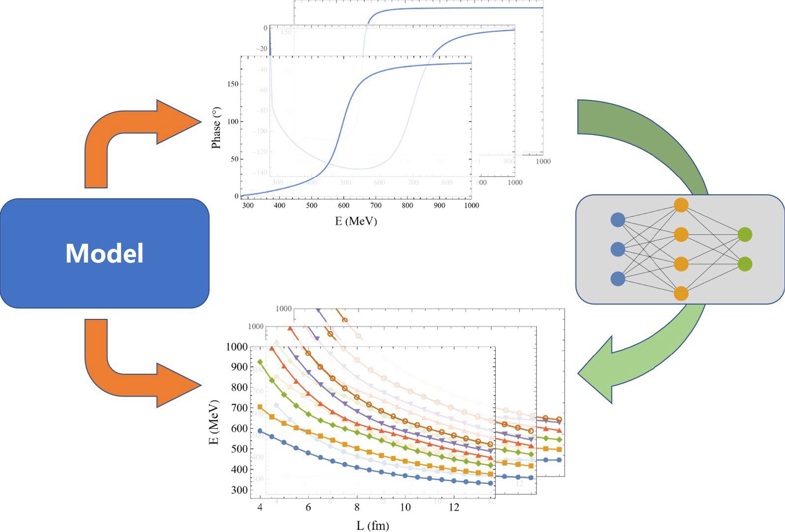
Figure 1.  (color online) The workflow of this work.

One successful approach to address this issue is called Lüscher's formula [14–16], developed by Lüscher and collaborators more than 30 years ago. By making use of the finite volume effects, Lüscher's formula describes relation of the spectrum $ E(L) $ of a two-body system on the finite lattice of size L with the scattering phase shift $ \delta(E) $ of this system in the continuum Minkowski space. The extension of Lüscher's formula to three-body systems is still undergoing [17–27]. Lüscher's formula and its extension are not only practically useful, but also is invaluably model-independent on the theoretical side. Deriving these model-independent theoretical approaches are very challenging and require a lot of wisdom and insight.

For the multi-channel case, more than one free parameters in the scattering amplitude will show up in the infinite volume, while Lüscher's formula offers only one constrain to connect the volume size and scattering amplitude at the discrete energy levels. To extract the information of scattering amplitude in the infinite volume, we will need several different finite volume sizes which share the same energy level. However, one cannot know a priori which volume size will produce the desired spectra without doing the expensive lattice calculations. Therefore, one practical way in the multi-channel process is to build a model to relate the scattering amplitude at different energy levels in order to use the Lüscher's formula to translate the lattice spectrum into phase shifts or other information. As a consequence, model dependence will inevitably enter into such calculation. In contrast, since the neural network is trained via the data-driven way, it is naturally model independent, or at least its model dependence can be safely ignored. To this end, as a firs step, we should answer whether the neural network can rediscover the numerical Lüscher's formula in single channel case.

Another challenge comes from the Lüscher's formula itself. Unlike extracting the analytic expression of the conserved quantities from the trajectory by ML approach [4], the Lüscher's formula is beyond the elementary function, therefore it can only be evaluated numerically. This property also leaves a great challenge for neural network to discovery it.

Encouraged by the achievement of machine learning in various areas, it is intriguing to ask if the neural network is able to discover the Lüscher's formula and its variance after fed by plenty data of spectra on lattice and the corresponding phase shifts. If a model-independence link does exist, in principle, a highly generalizable neural network will be a decent approximation of this link, because of the universal approximation theorem [28–30]. In this paper, we will show that neural network is able to rediscover the numerical Lüscher's formula to a high precision.

This paper is organized as follows. Sec. II is devoted to build the theoretical formalism to generate the data of energy levels in the finite volume and phase shifts in the infinite space. Then we will elaborate on the construction of neural network and its training setup in Sec. III. In Sec. IV, we will analyse the result in detail, and provide the evidence to show the numerical form of Lüscher's formula is generated from neural network. Finally, we give a brief conclusion in Sec. V.

It is known that Lüscher's formula connects the finite volume energy level E and the S-wave phase shift $ \delta(E) $ as [16]

where $ q=\dfrac{k_{0} L}{2 \pi } $ is defined with $ k_0 $ being the on-shell momentum of energy E, and the generalized zeta function $ {\cal{Z}}_{00}(1;q^2) $ is defined as

The system which we check against Lüscher's formula is the elastic $ \pi\pi $ S-wave scattering process. In order to generate the training and test set, which consists of the phase shift $ \delta(E) $ and the finite volume spectrum $ E(L) $ for a given lattice size L, we model this scattering process by Hamiltonian Effective Field Theory (HEFT) [31].

Following Refs. [32, 33], we assume that $ \pi\pi $ scattering can be described by vertex interactions and two-body potentials. In the rest frame, the Hamiltonian of a meson-meson system takes the energy-independent form as follows,

The non-interacting part is

where $ |\sigma\rangle $ is the bare state with mass $ m_{\sigma} $, and $ |\vec{k}\rangle $ is for the $ \pi\pi $ channel state with relative momentum $ 2\vec{k} $ in the rest frame of σ, and $ \omega(k)=\sqrt{m_\pi^2+k^2} $.

The interaction Hamiltonian is

where $ \tilde{g} $ is a vertex interaction describing the decays of the bare state into two-pion channel,

and the direct $ \pi\pi \to \pi\pi $ interaction (only S-wave) is defined by

For the S-wave, the $ \pi\pi $ scattering amplitude is then defined by the following coupled-channel equation,

where the coupled-channel potential is

We choose the normalization $ \langle \vec{k}|\vec{k}^{'}\rangle = \delta (\vec{k}-\vec{k}^{'}) $, such that the S-matrix (and thereby the phase shift $ \delta(E) $) in each partial-wave is related to the T-matrix by

with

and $ 2\omega(k_{on})=E $.

On the other hand, the HEFT provides direct access to the multi-particle energy eigenstates in a periodic volume characterized by the size length L. The quantized three momenta of the π meson is $ k_n = \sqrt{n}\dfrac{2\pi}{L} $ for $ n = n_x^2+n_y^2+n_z^2 $ where $ n_x, n_y, n_z=0,\pm1,\pm2, \ldots $. Then the Hamiltonian matrices with discrete momenta are,

The corresponding finite-volume matrix elements are given by

where the factor $ C_3(n) $ is the degeneracy of $ (n_x, n_y, n_z) $ that gives the same n. The factor $ \sqrt{\dfrac{C_3(n)}{4\pi}}\left(\dfrac{2\pi}{L}\right)^{3/2} $ follows from the quantization conditions in a finite box of a size L, where only S-wave contribution is included. With this Hamiltonian matrix, the spectra in the finite volume are the eigenvalues $ E(L) $ of H satisfying $ H|\Psi_E\rangle = E(L)|\Psi_E\rangle $.

For $ g(k) $ and $ v(k,k') $, we let them to be

and in order to explore different types of data, three different forms of the $ f(a;k) $ and $ u(a;k) $ is assumed,

which are model A, B and C, respectively.

Note that the shapes of the potentials in the momentum space become sharper and sharper from model A to model C. Since a sharper potential in momentum space has a larger effective range in coordinate space, and therefore has a more prominent finite volume effect, which is an artifact of a finite lattice. This artifact can be attributed to the deviation of the discrete momentum summation from the continuous momentum integration of the kernel function of the model. It is proved that the finite volume correction to Lüscher's formula behaves as $ e^{-m L} $ with m being the typical energy scale of the model and a sharper potential will suffer larger corrections in general.

To ensure the diversity of the data, the training set should cover both the broadest and the sharpest potentials. In practice, the data from model A and C are used as the training set, while the data from model B serve as the test set. Each data set includes 100 evenly-sampled phase shift $ \delta(E) $ values from $ 2m_\pi \approx 277{\rm{MeV}} $ to $ 1{\rm{GeV}} $, and the lowest 10 energy levels of $ E(L) $ for different lattice sizes $ L\in [10,13] $ fm with a step size $ 0.5 $ fm. The parameter space is spanned by $ m_\sigma({\rm{MeV}}),g_{\sigma},c({\rm{fm}}),g_{\pi \pi} $ and $ d({\rm{fm}}) $, ranging from $ [350,700] $, $ [0.5,5] $, $ [0.5,2] $, $ [0.1,1] $, $ [0.5,2] $, respectively. The space is randomly sampled by 2500 points for each model A, B and C. Once the parameters are fixed, we calculate the phase shift $ \delta(E) $ in continuum space and $ E(L) $ for lattice size L in $ [10, 13] $ fm with step size $ 0.5 $ fm. The phase shift $ \delta(E) $ is evenly sampled by 100 points from $ 2m_\pi \approx 277 $ MeV to $ 1 $ GeV, and the lowest 10 energy levels of $ E(L) $ were kept for training and testing.

We summarize the workflow and the structure of the neural network in Fig. 2. Since the phase shift $ \delta(E) $ contains the full information of a scattering process, it is natural to expect that the finite volume energy $ E(L) $ can be predicted from $ \delta(E) $. This is treated as a feature extraction task. To be precise, for a given phase shift $ \delta(E) $ and a lattice size L, the neural network is designed to predict the lowest 10 energy levels $ E(L) $ above the $ \pi\pi $ threshold. With some trial-and-error, we construct a small feed-forward fully-connected neural network with “SoftPlus" activation function. The neural network is trained by ADAM method, with learning rate $ 10^{-3} $ and batch size $ 10^4 $. 10% of the training set is kept for validation and training process finishes after $ 4\times 10^4 $ epoch.

Figure 2.  (color online) The structure of our neural network. Green round rectangles with integer n represent the linear layer with size n, which consists of all the learning parameters. Orange circles denote the input and output nodes and blue circles are layers with operations marked in the middle. The yellow thick arrow marks the “SoftPlus” activation function and the right brace is a conjunction of the corresponding layers.

In Fig. 2, L and $ \delta(E) $ are fed separately into different ports, since they are different physical quantities ($ \delta(E) $ has nothing to do with L). In order to speed up the training, we also normalize the input $ \delta(E) $ by dividing $ 360 $ and output $ E(L) $ by multiplying $ 1000 $. Instead of the widely used rectified linear unit, we also find our task prefers more smooth activation functions, such as “SoftPlus“. Although a strict proof is still missing, we speculate this preference of smooth activation functions originates from the regularity or even analyticity of the formulas in physics. Compared with the tiny neural network such as LeNet-5 in computer vision [34], our network is even smaller. However, it turns out that such a simple network is already adequate to make notable predictions.

For a regression task, one natural test is to calculate the deviation $ \Delta(E)=E_{{\rm{model}}}-E_{{\rm{NN}}} $ of the neural network prediction $ E_{{\rm{NN}}} $ from the ground truth values $ E_{{\rm{model}}} $ from models.

As shown by the histograms in Fig. 3, $ \Delta(E) $s of all the three models cluster around zero which ensures the precision of the neural network. It is also reasonable to see the precision on the test set (model B), is slightly worse than that of the training set (model A and C).

Figure 3.  (color online) The histogram of $ \Delta(E)\equiv E_{{\rm{model}}} - E_{{\rm{NN}}} $ at $ L=10 $ fm, where $ E_{{\rm{model}}}, E_{{\rm{NN}}} $ represent the predictions from the neural network and the model, respectively. The neural network is trained on the data from model A and C, and the data from model B serves as test set.

For the test set, there is an additional feature in Fig. 3: The distribution of $ \Delta(E) $ has a slightly heavier tail on the right. This implies that $ E_{{\rm{NN}}} $ is generally smaller than $ E_{{\rm{model}}} $. It turns out, this systematic underestimation of the spectrum is not a flaw of neural network, on the contrary, it reveals that neural network is successfully trained as a decent model-independent feature extractor which essentially approximates the Lüscher's formula.

To see this, we plot the Lüscher's formula along with the model predictions in Fig. 4, where we insert the spectrum back to the phase shift and make a scattering plot of $ [E_L, \delta(E_L)] $.

Figure 4.  (color online) Comparison of the Lüscher's formula (red), predictions from the neural network (black) and models (blue), where lattice size is 10 fm.

By definition, these points should agree with the Lüscher's formula up to a model-dependent correction term $ e^{-mL} $. Theoretically, it is difficult to foreseen the magnitude or even the sign of this correction term.

As shown in Fig. 4, data from model A are nearly identical to what Lüscher's formula predicts. This agrees with what we have anticipated, since the potentials in model A are generally narrow in coordinate space, the correction terms are small. Compared with this ideal-matching case, data from model C becomes much nosier. However, the mainstream of it still agrees considerably with Lüscher's formula, and the blue points are evenly scattered along two sides of red curves. It can also be seen in Fig. 5 that, with the increase of the volume size, the model becomes closer to the Lüscher's formula predictions.

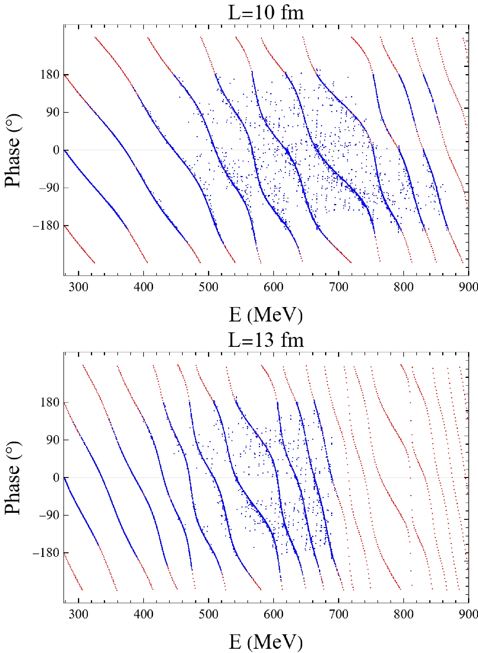
Figure 5.  (color online) Comparison of model C (blue points) with the Lüscher's formula in different volume sizes.

Compared with model A and C, a new feature from the model B is that the spectra from the model are systematically larger than what Lüscher's formula have predicted. Thus, if the neural network learns the Lüscher's formula well, spectra from model B will be naturally larger than neural network predictions.

The above statement can also be confirmed by comparing the two plots of the second column in Fig. 4. After training, the neural network suppresses the energy levels towards what Lüscher's formula predicts when it applies on model B, thus leading to a less accurate results and notable non-central distribution in Fig. 3. Thus, the deviation on model B signifies that neural network successfully captures the model-independent ingredients in the process $ \delta(E) \to E(L) $ and effectively treats the model-dependent features as noise.

We speculate that this may partially due to the small size of the neural network (28362 parameters V.S. $ 3.5*10^5 $ energy points + $ 5*10^5 $ phase shift points in training set), which keeps the neural network from learning or even memorizing the highly model-dependent feature (see. e.g. Ref. [35] for the risk when the number of parameters exceeds the number of data points). Since Lüscher's formula is the only model-independent approach, this lead to our central conclusion that we get a neural network reprint of the numerical Lüscher's formula.

To make a stronger evidence that the numerical Lüscher's formula is learned by neural network, it is necessary to expand the test set and explore the generalizability further, i.e., challenge the neural network by more different types of phase shifts. This will not only reveal more interesting structure of the neural network, but also guide us to spot a subtle deficiency in the above treatment.

One typical pattern of the phase shift $ \delta(E) $ in our training and test set is that, with the increase of energy, $ \delta(E) $ will departure from zero at $ 2m_\pi $ threshold, gain a sharp or broad resonance structure in the middle steps and end up to be $ 0^\circ $ or $ \pm 180^\circ $. Here, we will challenge the neural network by feeding a constant phase shift $ \delta(E)=\delta_0 $, where $ \delta_0 $ ranges in $ [-180^\circ, +180^\circ] $. Since this constant phase shift is far beyond our training set, it would be impossible to pass the test if the neural network were doing nothing but a trivial memorization.

In Fig. 6, the agreement between Lüscher's formula and neural network is even more fascinating except an unexpected twist around $ \delta=0^\circ $. To be precise, if we track the lowest level of the spectrum $ E_1 $, the neural network concludes from the data that $ E_1 $ should generally increase with the decrease of $ \delta_0 $. However, once $ \delta_0 $ crosses the zero from above, another lower energy level will emerge. Thus, as a function of $ \delta_0 $, $ E_1 $ is not a continuous function at zero. This discontinuity is essentially caused by the periodicity of the phase shift: $ \delta(E) $ and $ \delta(E) + n\pi $ corresponds to the same physics. On the other side, since the neural network is designed to predict the lowest 10 energy levels above the threshold, and the activation functions are continuous in order to do back-propagation in the training process, the best neural network can achieve is to make a soft transition between the neighbor red curves around $ \delta_0=0^\circ $, resulting several zigzag tracks in Fig. 6. It is also worthy to find that this twist structure does not manifest itself in Fig. 4, which makes this constant-phase-shift-test valuable.

Figure 6.  (color online) Prediction (black dots) from the neural network when phase shift is constant $ \delta(E)=\delta_0, \delta_0\in [-180^\circ,180^\circ] $. The precise Lüscher's formula curve is marked as red dots. One period boundary $ \pm 90^\circ $ is marked by gray horizontal line for comparison.

We circumvent this twist issue by the following approach. The energy level E is marked as $ E_1 $ only when $ \delta(E) $ is negative and $ E<2\sqrt{\left(\frac{2\pi}{L}\right)^2 +m_\pi^2} $, otherwise, the valid energy levels starts from $ E_2 $. Noting that this does not request any pre-knowledge of the Lüscher's formula. It is essentially a convention that $ \delta(E) $ is zero at the following free energies

where $ \vec{n}=(n_x,n_y,n_z), n_{x,y,z}=0,\pm 1,\pm 2,\ldots $. Retraining the neural network with the above modification results in a superb agreement with the Lüscher's formula, which is shown in Fig. 7. The slightly worse precision around $ \pm 180^\circ $ can be improved by either increasing the size of the neural network or we can simply ignore the neural network predictions by constraining it within a period, such as $ [-90^\circ,+90^\circ] $ and extrapolate the results to other regions by periodicity. After addressing this twist issue, we finally strengthen the previous conclusion that the numerical form of Lüscher's formula is learned by the neural network.

Figure 7.  (color online) Same as Fig. 6, with energy level issue explicitly addressed.

In this paper, we have shown that the numerical form of Lüscher's formula can be rediscovered by the neural network when it is trained to predict the spectrum on lattice from the phase shift in continuous space. From the perspective of pragmatism, the neural network is able to exploit the sophisticated data and extract valuable information. In a broad sense, our work is an concrete example to demonstrate how to extract model-independent link between model-dependent quantities in a data-driven approach. Surprised by the capability of the neural network, we believe its potential is still waiting for physicists to explore.

We are grateful to Yan Li, Qian Wang, Ross D. Young and James M. Zanotti for useful discussions.