Study the yrast and yrare low-lying excited states using machine learning approaches

The investigation of the properties of nuclear excited states is crucial for elucidating the complex interactions of protons and neutrons in atomic nuclei. While substantial progress has been made in characterizing low-lying yrast and yrare states of nuclei near the stability line, experimental measurements remain particularly scarce for nuclides that are close to or beyond the drip lines [1−13]. The measurement of excited states unveils the wide diversity of nuclear phenomena, e.g., shell evolution, pairing correlation, shape coexistence, octupole deformation, clustering, continuum effects [14−18]. Currently, a vast number of exotic nuclei have yet to be measured due to the challenges posed by various experimental techniques and the considerable investment of beam time required, primarily because of their low production cross section. Among the excited states, the $ 2_1^+ $ state garners significant attention because of its fundamental importance, carrying crucial benchmark information for investigating the evolution of shell structure and collectivity. As the proton and neutron numbers approach the magic numbers, the energy of the $ 2_1^+ $ state, $ E(2_1^+) $, increases sharply, reaching a maximum in double magic nuclei. As one moves away from the magic numbers along isotope chains, the presence of low $ 2_1^+ $ excitation energies reflect deformed ground state stem from the polarizing effect of added nucleons, which induces deformation. The non-yrast $ 2_2^+ $ states are regarded as indicators of collectivity, showing simpler characteristics compared to their $ 2_1^+ $ counterparts. The physical properties of $ 2_2^+ $ excited states are always of interest due to their potential role as initial levels of collective bands, which are traditionally referred to as γ-vibrational bands or quasi-γ bands.

Various theoretical methods have been developed to reproduce and predict the energies of low-lying excited states, as well as further to explore their underlying physical mechanisms over the Segrè chart, e.g., shell model [19, 20], nuclear energy density functional theory [21−24]. However, these models often demand a large amount of computational resources, and notable discrepancies between the model calculations and experimental data have been observed for nuclei located far from the stability line [25−27]. This may be attributed to the complexity of the mapping function, which is non-trivial and, in some cases, cannot be properly defined. In recent years, machine learning (ML) algorithms have been used to simulate known data and predict unmeasured ones [28−31]. It has been shown that ML achieves significantly shorter computation times than traditional methods while maintaining comparable accuracy. Promising results have been obtained using ML to address critical issues and predict unknown properties of nuclei [28−30], e. g., β-decay half-lives and energy [32−36], α-decay [37−41], mass and charge radius of atomic nuclei [42−45], nuclear density distribution [46−49], heavy ion collisions [50−53]. Recently, the energies of the $ 2_1^+ $ states were studied using the Bayesian neural network (BNN) approach, artificial neural networks method, and machine leaning approach for even-even nuclei across the nuclide chart, showing superior performance compared to the shell model and the five-dimensional collective Hamiltonian model [54−57].

In this study, two types of algorithms are employed to investigate the excitation energies of $ 2_1^+ $ and $ 2_2^+ $ states: the Light Gradient Boosting Machine, which is based on decision trees, and Sparse Variational Gaussian Process, which is a Bayesian method. Both algorithms are supervised tasks that require ML algorithms along with a set of labeled data consisting of input and output variables for regression predictions. Our goal is to assess the performance of the two ML algorithms in predicting the $ E(2_1^+) $ and $ E(2_2^+) $, and to also examine their interpretability. In addition, the present study aims to extrapolate these observables to unseen data, rather than merely optimizing the fit to known data by minimizing the root-mean-square (rms) error. A comparison with the calculated results using the Hartree-Fock-Bogoliubov theory extended by the generator coordinate method and mapped onto a five-dimensional collective quadrupole Hamiltonian (HFB+5DCH) is also presented [25]. It is noteworthy that although $ E(2_1^+) $ has been studied using other machine learning approaches, it is intriguing to explore whether new algorithms can refine the predictions, thereby facilitating more reliable explorations of unmeasured nuclei. In addition, the present work is the first attempt for the exploration of $ E(2_2^+) $ within the framework of machine leaning. Finally, the performance of these ML models in predicting $ E(2_1^+) $ and $ E(2_2^+) $ was also examined using 12 newly measured data points that were not included in the training set.

The article is organized as follows: Section II describes the LightGBM and SVGP algorithms, training and testing datasets, as well as the input features. The obtained results from the two algorithms and discussions are presented in Section III. In Section IV, we summarize our findings and conclusions from the present work.

In this section we introduce the two algorithms employed in our study: Light Gradient Boosting Machine and Sparse Variational Gaussian Process. We also outline the parameter sets, training and validation datasets used in these models.

LightGBM as an efficient gradient boosting framework developed by Microsoft that has been widely used for various machine learning tasks [58]. It employs a histogram-based learning algorithm that significantly accelerates training and reduces memory usage compared to traditional boosting methods. LightGBM handles sparse data and categorical features effectively, supports parallel and distributed computing, and performs well in tasks such as classification, regression, and ranking. A key advantage of LightGBM lies in its optimized leaf-wise tree growth strategy, which improves accuracy by reducing loss more aggressively than level-wise methods. Combined with its strong scalability and low computational cost, LightGBM has become a popular choice in both machine learning competitions and real-world applications.

SVGP is a scalable probabilistic modeling approach that integrates variational inference with sparse approximations [59, 60]. By introducing a small set of inducing points, SVGP reduces the computational complexity of standard Gaussian Processes (GP) from $ {\cal{O}}(N^3) $ to $ {\cal{O}}(M^3) $, where $ M \ll N $, while preserving core GP properties such as uncertainty quantification. Its main strengths include: (1) Efficiency, through sparse matrix operations and evidence lower bound (ELBO) optimization; (2) Flexibility, supporting non-Gaussian likelihoods, high-dimensional features, and customizable kernels; and (3) Interpretability, as the variational distribution $ q(u) $ directly conveys the model’s confidence in predictions. Compared to traditional GPs and deep neural networks, SVGP offers a balanced trade-off between expressiveness, uncertainty estimation, and computational feasibility, serving as a bridge between Bayesian inference and large-scale machine learning.

To ensure fair and effective model evaluation, key hyperparameters for both models were systematically configured, with an emphasis on balancing predictive accuracy and computational efficiency. For LightGBM, the main hyperparameters are set as follows: the maximum number of leaves per tree is 10, the maximum depth is set to -1 (indicating no depth limit), and the number of boosting iterations is fixed at 50,000. All other parameters remain at their default values to maintain standard model behavior. For SVGP, the number of inducing points (n_z) is set to 100 to enable sparse variational approximation. During training, 20 particles (n_particles = 20) are used for Monte Carlo estimation of the ELBO, and 100 particles (n_particles_test = 100) are used during testing to improve stability. The model is trained using a batch size of 300 (batch_size = 300) over 8000 epochs (n_epoch = 8000), with a learning rate of 0.01 (lr = 0.01).

The dataset used in this study comprises a total of 660 and 437 experimental data points corresponding to the excitation energies of the $ 2_1^+ $ and $ 2_2^+ $ states, respectively, in even-even nuclei with proton numbers ranging from $ Z = 10 $ to $ Z = 100 $. The data are obtained from the National Nuclear Data Center [61]. To train the machine learning models, the dataset is randomly divided into training and test sets with various ratios. In our previous work, we initially investigated the effect of the ratio between the training and validation sets on the prediction performance of the LightGBM model [56]. The results showed that the rms deviation decreases as the proportion of training data increases. However, an excessively large training set reduces the number of data points in the test set, thereby increasing the uncertainty of performance evaluation. Therefore, following the set in earlier studies, we adopt a split ratio of $ 80 $% for training and $ 20 $% for validation in this work. This 4:1 division, along with other commonly used ratios such as 7:3 or 3:1, is a standard strategy widely applied in machine learning model design. Totally, we randomly divide the data points into training and validation data sets 500 times. In order to study $ E(2_1^+) $ and $ E(2_2^+) $, we incorporate 16 relevant features of nuclei into our algorithm, referred to as $ M16 $. $ M16 $ consists of 16 inputs: one-proton separation energy ($ S_p $), one-neutron separation energy ($ S_n $), two-proton separation energy ($ S_{2p} $), two-neutron separation energy ($ S_{2n} $), and the separation energy of $ ^4 {\rm{He}}$ ($ S_{He} $); deformation parameters derived from FRDM calculations [62] ($ \beta_1 $) and from WS4 [63] ($ \beta_2 $); proton number $ (Z) $, neutron number $ (N) $, mass number $ (A) $, experimental binding energy (B), binding energy predicted from the liquid drop model ($ B_{LDM} $), the difference between experimental B and the liquid drop model ($ B-B{_{LDM}} $), Casten factor $ (P) $ [64], the valence number of neutrons as measured from the nearest closed shell ($ {\rm{v}}_n $), the valence number of protons as measured from the nearest closed shell ($ {\rm{v}}_p $). These features are recognized as fundamental characteristics of nuclei and impact the performance of ML models. The performance of ML algorithms on both training and test datasets were quantified using the standard rms deviation between the machine learning predictions and the experimental data, defined as follows:

where $ log_{10}E^{ML} $ represents ML predictions, $ log_{10}E^{Exp} $ denotes the experimental value, and N is the total number of nuclei.

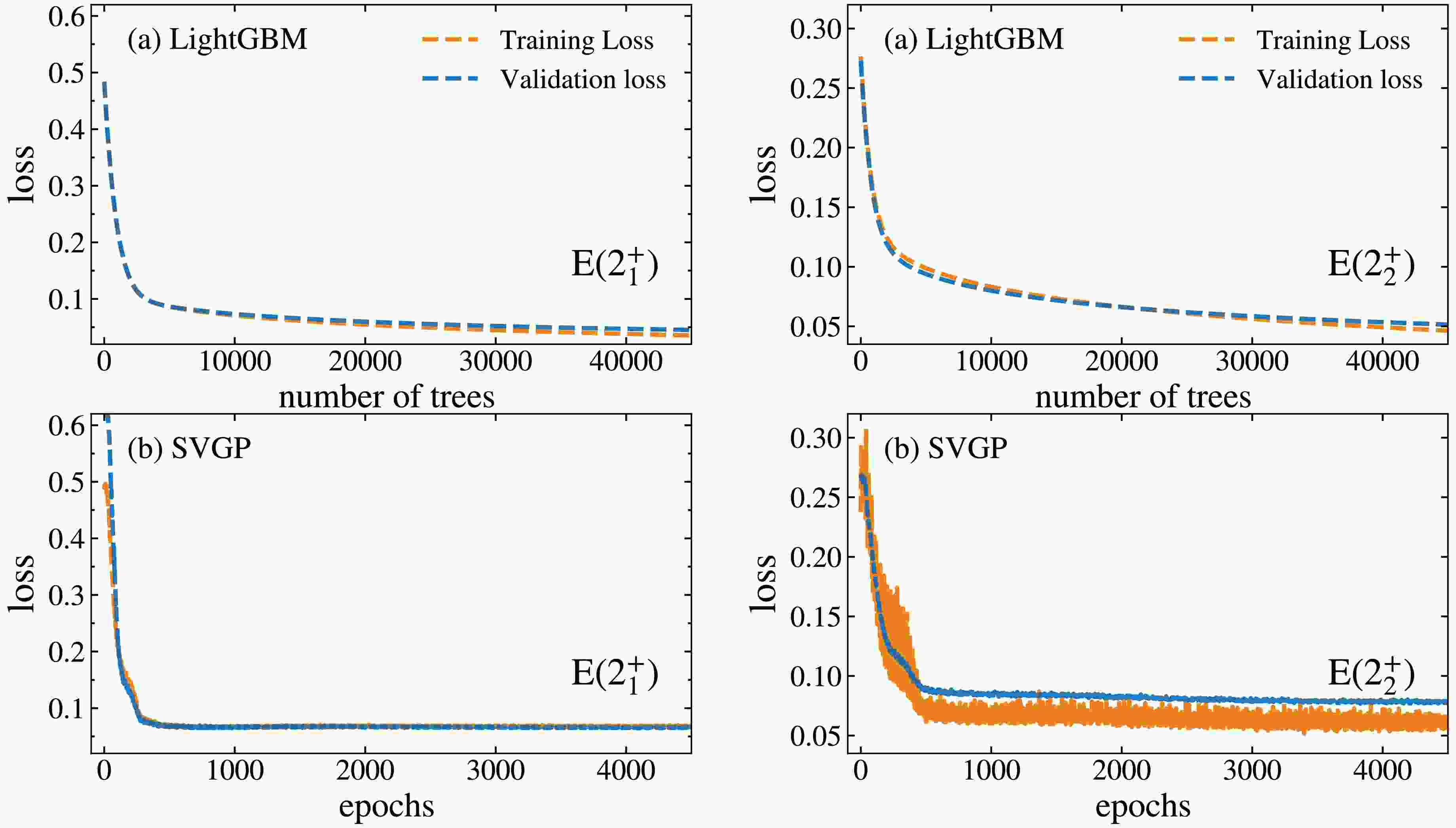
Performance of LightGBM and SVGP in the study of $ E(2_1^+) $. In this work, to ensure the quality the models, we initially examined the learning curves of LightGBM and SVGP for excitation energies of the $ 2_1^+ $ and $ 2_2^+ $ states under the 4:1 train-validation split, as shown in Fig. 1. The learning curves show how the loss function evolves with the number of training iterations (or trees). As training proceeds, the loss gradually decreases and converges, indicating that the model is approaching an optimal state. The difference between training and validation losses reflects model's fitting behavior: the two curves should be close under proper training, while a large difference between them suggests overfitting or underfitting. One can infer from Fig. 1 that the loss values for validation and training decrease with the increase in the number of trees (or epoches) and saturate at around 20000 for LightGBM and approximately 500 for SVGP in the study of $ E(2_1^+) $. For $ E(2_2^+) $, the saturation occurs at around 25000 for LightGBM and at around 500 for the SVGP, respectively. In addition, one can observe in Fig. 1, the loss functions for both models decrease steadily on both training and validation curves lying on top of each other, indicating no fitting issues. These results demonstrate that the selected hyperparameter configurations effectively ensure training stability, good generalization, and computational efficiency for both models.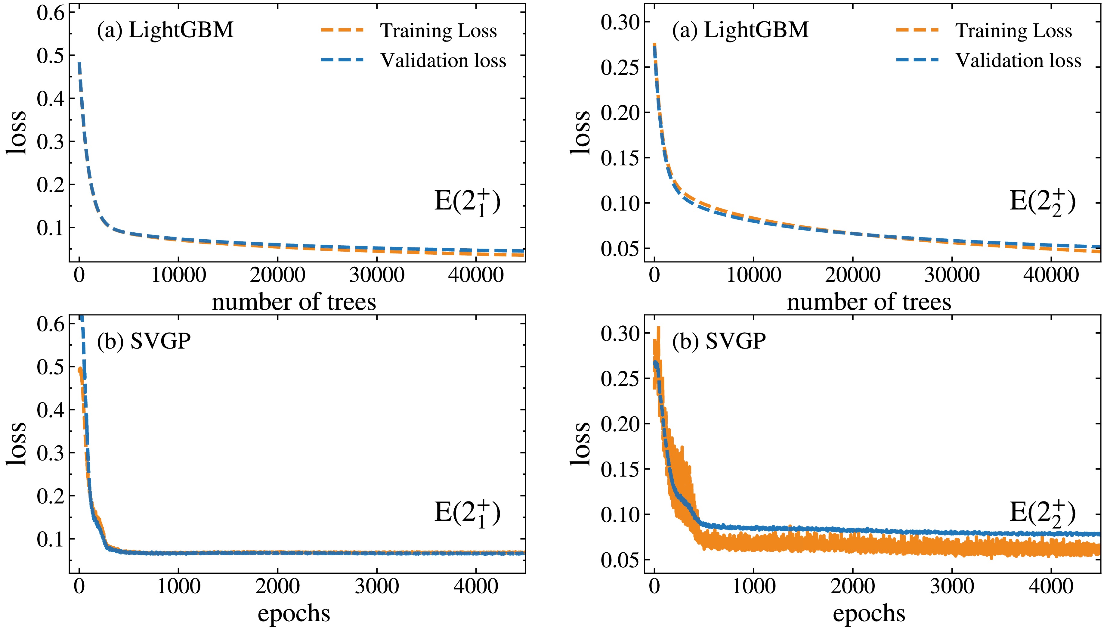

Figure 1.  (Color online) The learning curves of the LightGBM and SVGP models for the prediction of the excitation energies of $ 2^+_1 $ and $ 2^+_2 $ states illustrate the evolution of the loss function with training iterations (i.e., the number of decision trees or training epochs).

The excitation energies of the $ 2_1^+ $ states were previously explored in our work using the LightGBM algorithm [56]. The rms deviation of LightGBM approach with respect to the experimental $ {\rm{log}}_{10}E $ was determined to be 0.030(1) for $ E(2_1^+) $. In addition, the $ E(2_1^+) $ was also analyzed using LightGBM in Ref. [57], albeit with only five physical features. Nevertheless, it still revealed that the average difference between the LightGBM predictions and the experimental data was 18 times smaller than that obtained by the shell model and only $ 70 $% of the BNN prediction results [57]. In this study, we incorporated deformation parameters derived from FRDM calculations [62] ($ \beta_1 $) as an additional feature to account for the collectivity of nuclei. Finally, the rms values of 0.032(3) and 0.049(5) of the training and validation sets were obtained, respectively. By utilizing the same 16 input ($ M16 $) features within the framework of SVGP, we also investigated the $ E(2_1^+) $ of even-even nuclei. This implementation yielded rms values of 0.066(2) and 0.070(6) of the training and validation sets, respectively, which are a factor of two inferior to those obtained using LightGBM, suggesting that the LightGBM more effectively captures the excitation energies of $ 2_1^+ $ states.

Performance of SVGP and LightGBM in the study of $ E(2_2^+) $. Prior to this work, the excitation energies of $ 2_2^+ $ states remained unexplored using machine learning methodologies. In the current study, we employed LightGBM and SVGP to analyze $ E(2_2^+) $ using the $ M16 $ feature space. Fig. 2 illustrates the density distribution of the rms value for the validation dataset of the excitation energies of the $ 2_2^+ $ states using LightGBM and SVGP, respectively. The rms for the validation data points predicted by LightGBM and SVGP were 0.058(5), and 0.077(6), respectively. This means that LightGBM and SVGP reproduce the experimental data within a factor of $ 10^{0.058} = 1.14 $ and $ 10^{0.077} = 1.19 $, respectively. These results are better than that most of the traditional theoretical models. Similar to the study of $ E(2_1^+) $, the decision tree-based LightGBM outperforms SVGP in predicting $ E(2_2^+) $. For the reader's convenience, we have summarized the current results in Table 1. It is worth noting that although the predictions from LightGBM are deterministic under fixed training data and parameters, the reported validation rms error (e.g., $ 0.058 \pm 0.005 $) results from repeated random partitioning of the training data. Specifically, we performed 500 independent training runs, each using a randomly selected 80% of the data for training and the remaining 20% for validation. The reported mean value of rms and standard deviation are calculated across these runs to assess the model’s stability and generalization under different data splits.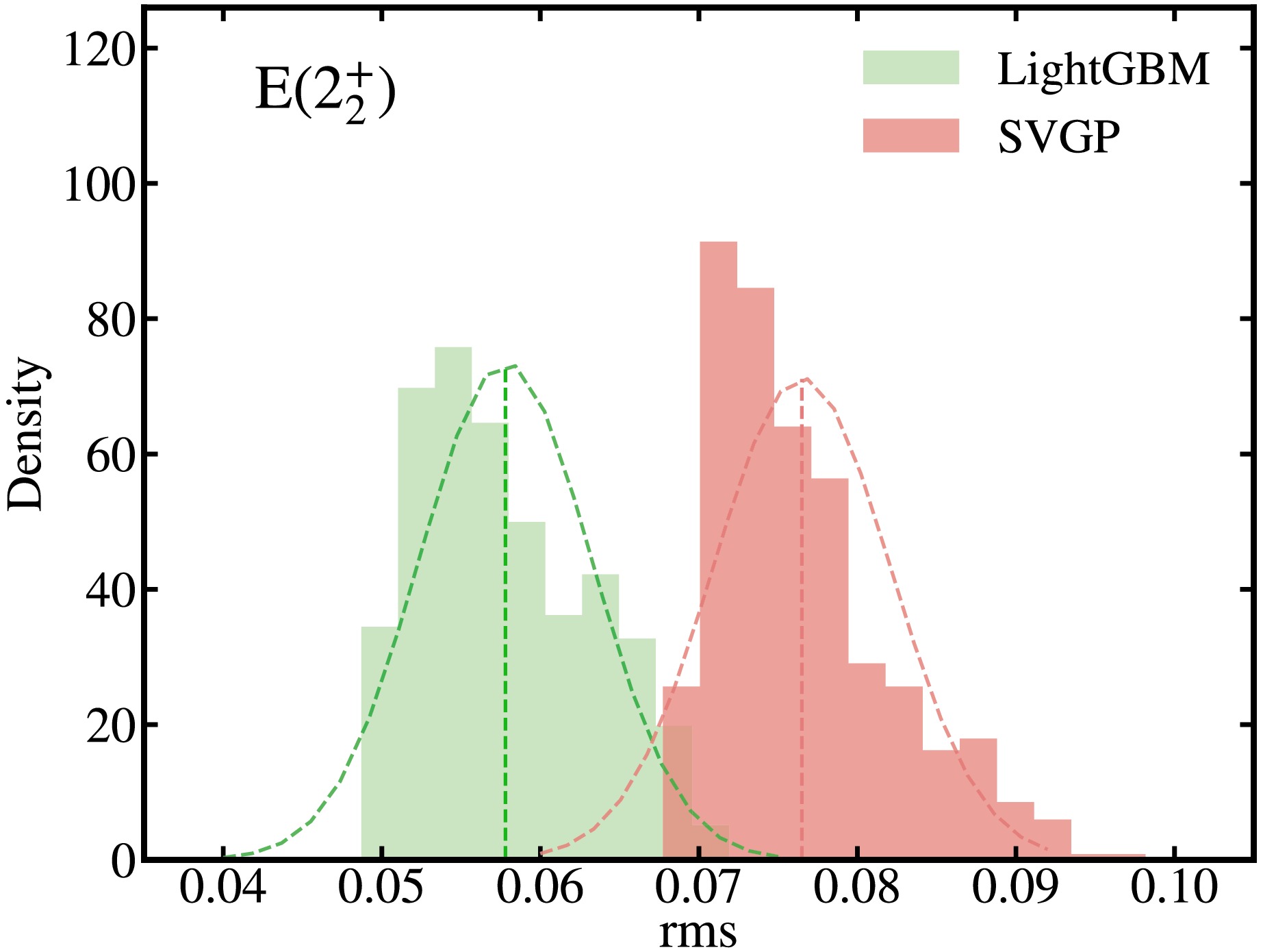

Figure 2.  (Color online) Density distribution of the rms value of the validation dataset from LightGBM and SVGP for the $ E(2_2^+)$ using M16 feature space, respectively. The results from 500 runs are displayed. Dashed lines denote a Gaussian fit to the distribution. In each run, the data points were randomly split into training and validation sets at a ratio of 4:1.

	Algorithms	Training	Validation
$E(2_1^+)$	LightGBM	0.032(4)	0.049(5)
$E(2_1^+)$	SVGP	0.066(2)	0.070(6)
$E(2_2^+)$	LightGBM	0.040(3)	0.058(5)
$E(2_2^+)$	SVGP	0.067(7)	0.077(6)

Table 1.  The average rms values on the training and validation sets.

Fig 3 displays the calculated excitation energies of the $ 2_2^+ $ states derived from LightGBM, SVGP, and HFB+5DCH calculations, as a function of their experimental values. This comparison facilitates a comprehensive evaluation of the predictive power of each methodology across an extensive energy scale, spanning over an order of magnitude from approximately 0.3 MeV to 10 MeV. The analysis reveals that, on average, the HFB+5DCH model tends to overestimate the excitation energies $ E(2_2^+) $, with predicted values approximately $ 25 $% higher than the experimentally observed ones [25]. In contrast, both SVGP and LightGBM exhibit reduced variance in their predictions, indicating greater consistency. Notably, the LightGBM predictions demonstrate a high degree of concordance with the experimental data, underscoring its superior accuracy compared to the HFB+5DCH and SVGP approaches.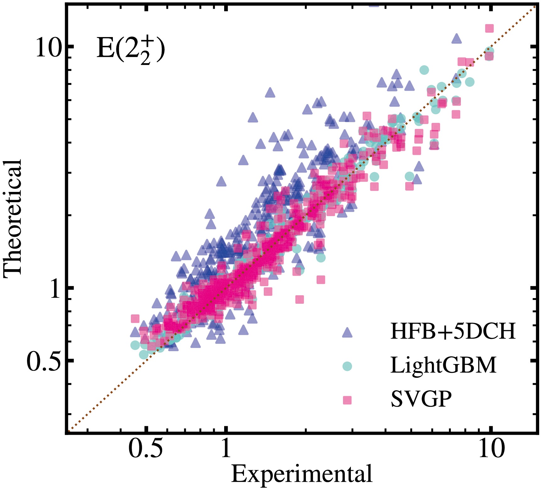

Figure 3.  (Color online) Theoretical results for $ E(2_2^+)$, obtained using HFB+5DCH, LightGBM, and SVGP, compared with the corresponding experimental data.

To more clearly illustrate the discrepancies between the calculations and experimental results, the differences between the machine learning predictions and experimental data for $ E(2_2^+) $ on the nuclear chart are quantified in Fig. 4. It is evident that both machine learning algorithms predictions exhibit excellent agreement with the experimental data for nearly all nuclei, including triaxial, transitional and magic nuclei. However, deviations are mainly observed in light nuclei with complex structures, presenting halos and clusters, as well as in these nuclei that exhibit dominant single-particle characteristics. Additionally, significant deviations are also noticeable in the neutron-rich nuclei of the medium-heavy mass regions, likely due to the relative scarcity of training data in these areas.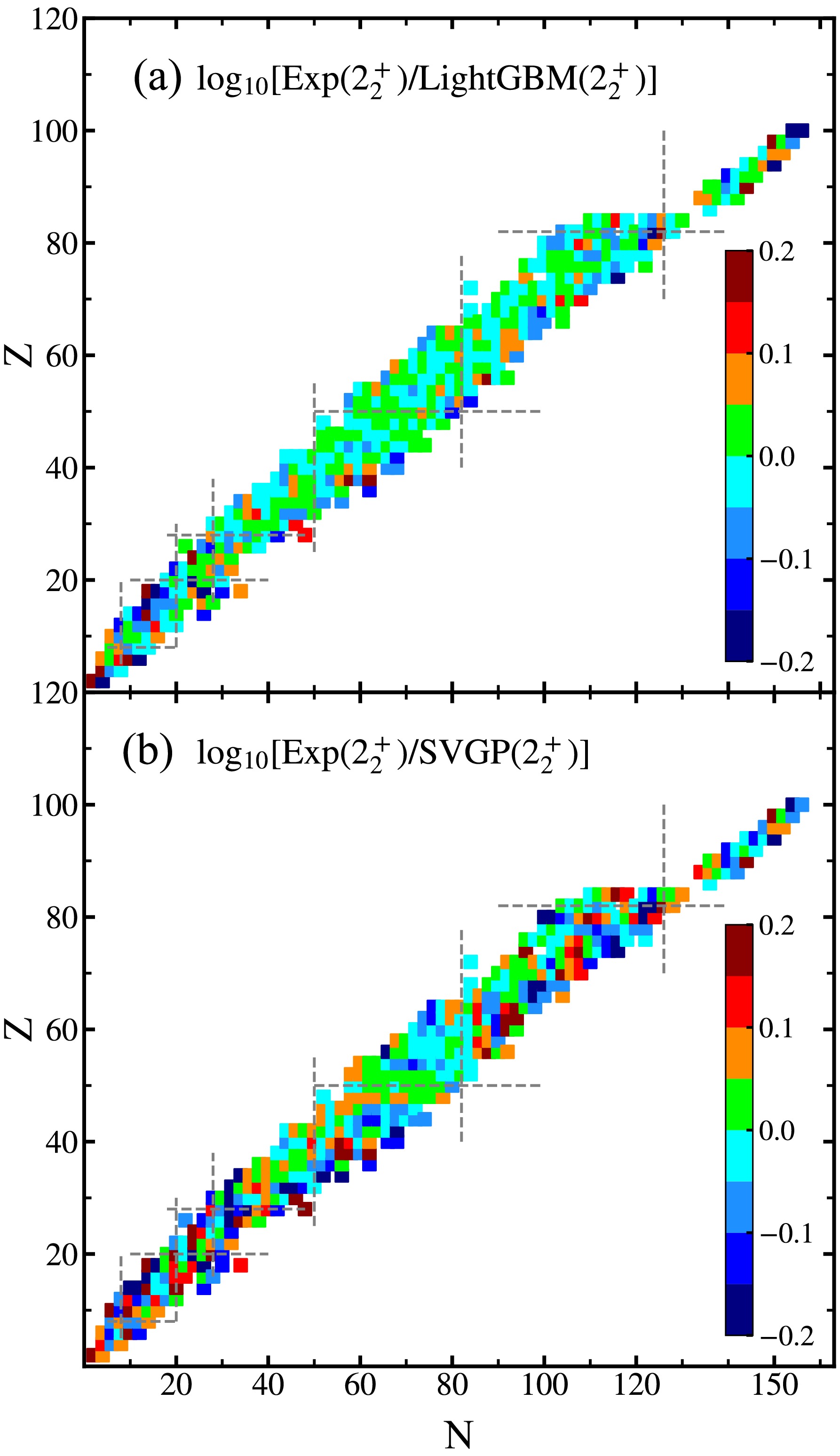

Figure 4.  (Color online) Panels (a) and (b) show the differences between the experimental data and machine learning predictions using LightGBM and SVGP for the excitation energies of $ 2_2^+ $ states, respectively.

Physically interpretablity. The implementation of machine learning algorithms is often constrained by their “black box” nature, which obscures the reasoning behind their predictions. Recently, explainable AI techniques have gained significant attention as critical tools for addressing the interpretability gap. Among various methods, SHapley Additive exPlanations (SHAP) has become widespread recognized for its effectiveness in providing clear, comprehensible insights into model behavior, while also quantifying feature importance through cooperative game theory frameworks [65−68]. In this work, we apply the SHAP technique to gain a deeper understanding of the results obtained from LighGBM. Fig. 5 presents the ranking of features obtained from the $ M16 $ feature space for predicting $ E(2_2^+) $ using LightGBM. In these plots, features are ordered along the y-axis according to their impact, with the most impactful feature at the top and the least influential at the bottom. The x-axis represents the relative importance of each feature, as determined by its SHAP value. Features with larger absolute SHAP values have a greater impact on the model’s predictions, while those with smaller values have a smaller effect. The analysis reveals that the feature P is the most critical, as it reflects nuclear collectivity, which was high sensitivity to $ E(2_2^+) $. A similar behavior of P was also observed for the study of $ E(2_1^+) $ [56, 57]. The difference in binding energy between experimental data and the liquid drop model (denoted as $ B-B_{LDM} $) occupies a secondary position in the ranking, reflecting shell and pairing effects, as well as nuclear deformation [56]. Following this, the top six features include Z, N, $ S_n $, $ S_{He} $. Beyond these, all other features have relatively smaller contribution, but it has indispensable contributions to the prediction of $ E_2^+ $. This suggests that using all 16 basic features appears a reasonable manner for making accurate predictions.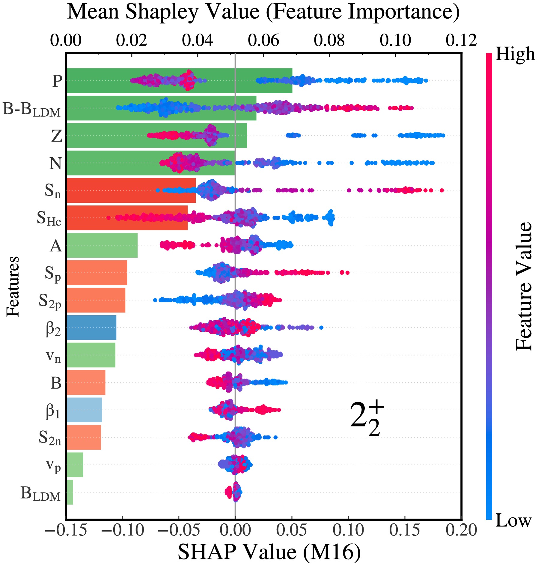

Figure 5.  (Color online) The ranking of feature importance measured by SHAP value for the excitation energies of $ 2_2^+ $ states. The color of each bar indicates the direction of the feature’s influence on the prediction: blue for a decrease with lower feature values and red for an increase with higher feature values, with the intensity of the color denoting the magnitude of the feature’s value.

To identify feature redundancy, we constructed a simplified feature set consisting of the top six SHAP-ranked features (denoted as M6) and used it as input to train both LightGBM and SVGP models. On the $ E(2_2^+) $ validation set, the resulting rms errors were 0.070 and 0.090, respectively—higher than the 0.058 (LightGBM) and 0.077 (SVGP) achieved with the complete M16 feature set. Compared to the M16 model, the rms values of the M6 models increased by approximately 20% and 16%, respectively, suggesting that non-linear interactions may exist among input features, and removing certain features could weaken the model's ability to leverage other information, ultimately impairing predictive performance.Therefore, although WS4’s $ \beta_2 $ ranked lower than FRDM’s $ \beta_1 $ in the SHAP analysis, we retained FRDM’s $ \beta_1 $ in the initial feature set to preserve any potential synergistic effects. Additionally, both LightGBM and SVGP have strong feature selection capabilities and employ regularization (LightGBM) and variational inference (SVGP) during training, making them robust to redundant features. This robustness underscores the reliability of our methodology and modeling choices.

Partial Dependence Plot (PDP) analysis is an another effective method for interrogating the functional relationship between input features and model predictions in the LightGBM algorithm [69, 70]. Within this framework, if the curve for a particular feature is nearly constant or shows random fluctuations, it suggests that the feature may be insignificant or uninformative. Conversely, a steep PDP curve or one that exhibits significant changes indicates that the feature has a substantial contribution to the model's predictions. Fig. 6 quantifies the impact of the six most salient input features on the prediction of $ E(2_2^+) $. Although PDP and SHAP utilize different techniques to characterize the importance, the identified six most important features are the same. Among the input features, proton number (Z) has the most pronounced influence on the prediction of $ E(2_2^+) $. It has a negative impact, an increase from 20 to 80 resulted in a decrease in the PDP value from 3.34 to 3.10, representing a reduction of approximately $ 7.1 $%. The Casten factor P also exhibits a negative impact, an increase from 0 to 4 resulted in a decrease in the PDP value from 3.29 to 3.08, representing a reduction of approximately $ 6.2 $%. Similar behaviors were observed for the features of N and $ S_{He} $. However, as shown in Fig. 6, the predicted $ E(2_2^+) $ increases with increasing values of $ B-B_{LDM} $ and $ S_n $. The effect becomes particularly significant when the difference in the binding energy ($ B-B_{LDM} $) increase from -3 to 3 MeV. As shown in Fig. 7, the PDP curve for $ B_{LDM} $ is nearly flat, with a variation of only about 0.16%, indicating a negligible average impact on the model’s output. This finding is consistent with its low importance revealed by the SHAP analysis..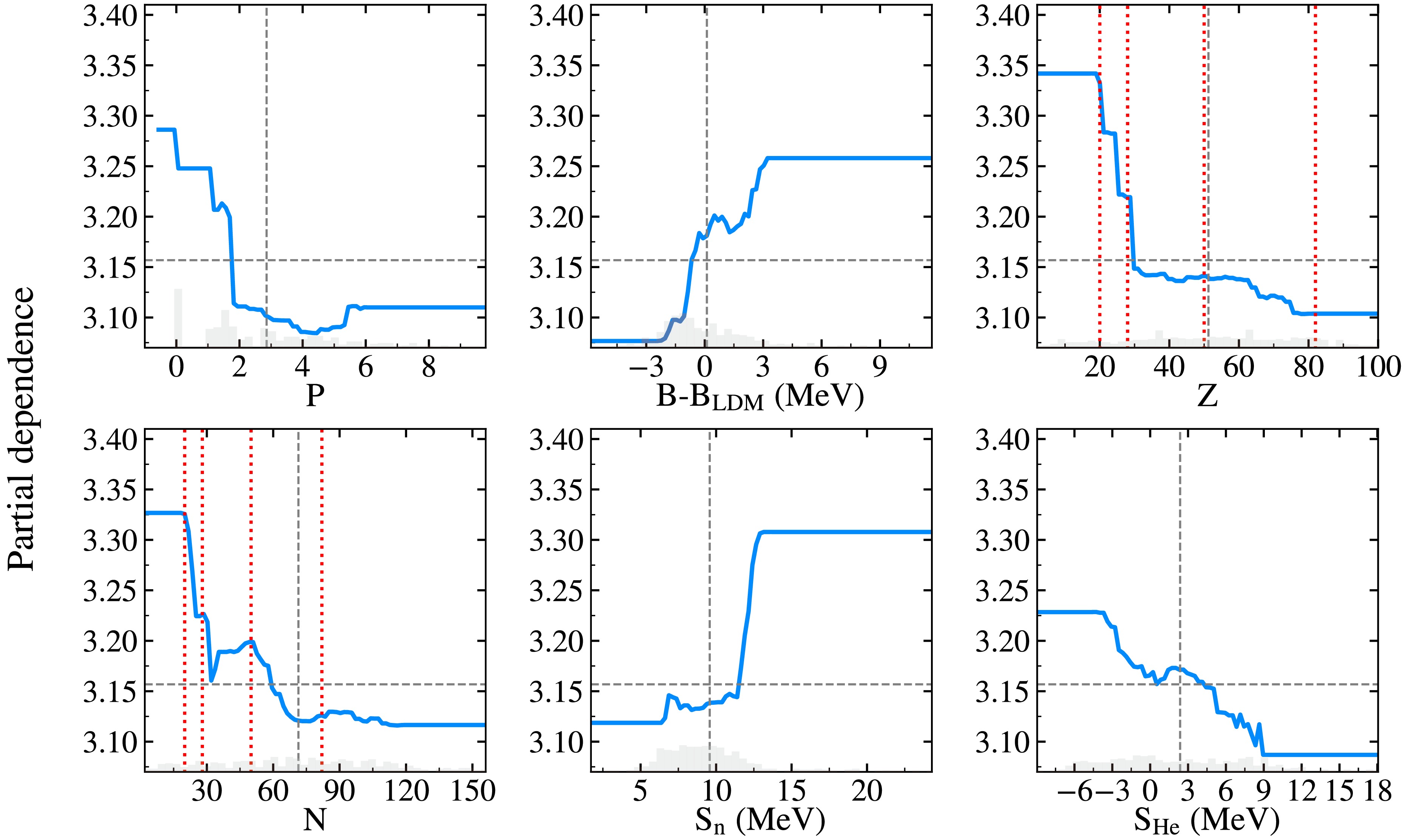

Figure 6.  (Color online) PDP analysis of the effect of input features on the excitation energies of $ 2_2^+ $ states. The blue lines represent the partial dependence value, while the gray columns represent the data point distribution for each input feature at a certain value. The red dashed lines indicate the positions of neutron or proton magic numbers.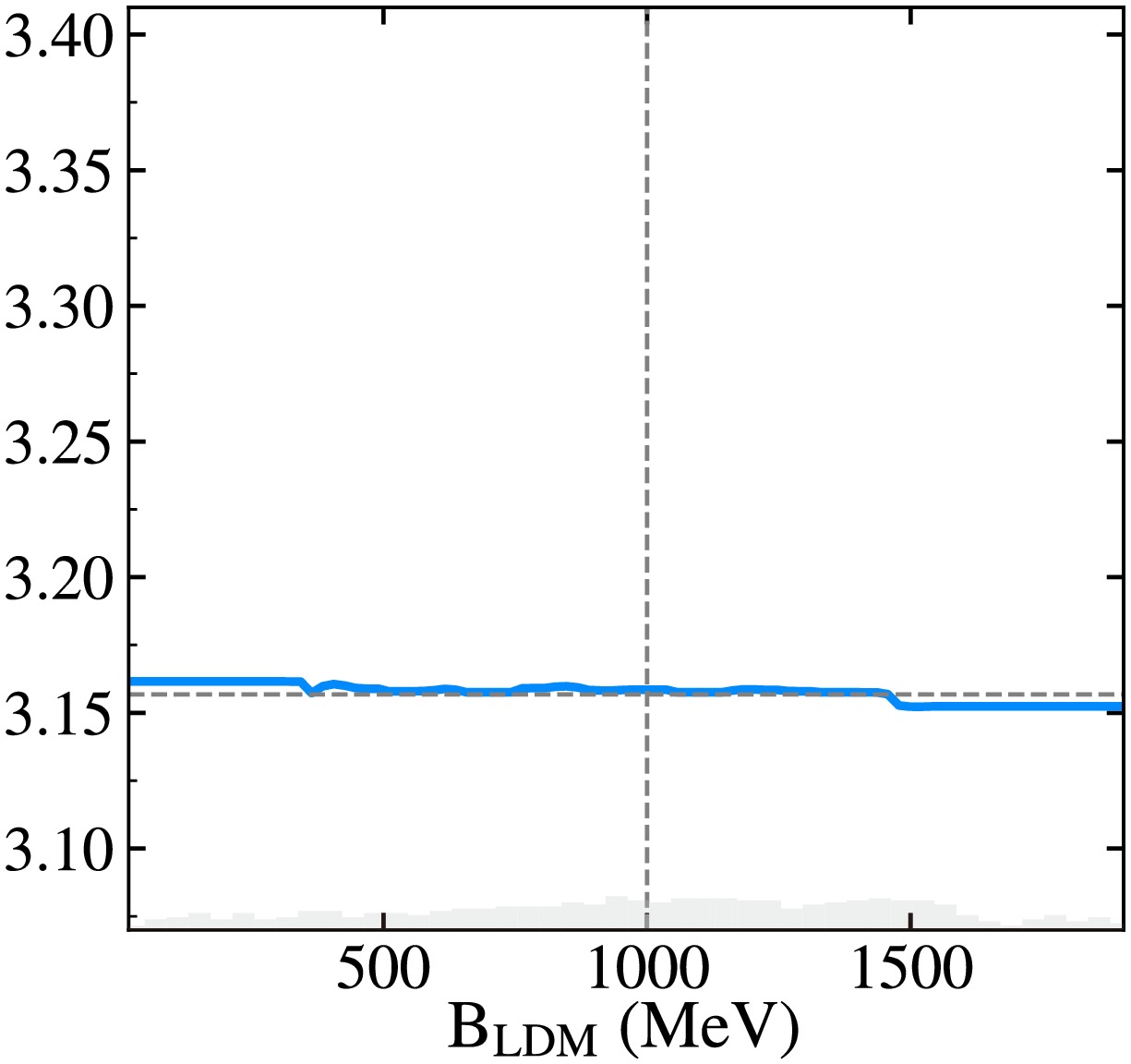

Figure 7.  (Color online) Similar to Fig. 6, but for $ B_{LDM} $.

Performance of SVGP and LightGBM on the newly reported data. In addition to best reproduce the known $ E(2_1^+) $ and $ E(2_2^+) $ data across the nuclear landscape, one of important objective of this work is to apply the algorithms in the extrapolated region where experimental measurements are absent or currently inaccessible. In present work, we initially evaluate the extrapolation abilities of the LightGBM and SVGP algorithms by venturing beyond the training area using new data points. Fig. 8 compares a total of 12 newly reported data from 2020 to the present with the predictions from LightGBM and SVGP [71−81]. These newly measured data points were not included in the training process. It is evident that LightGBM and SVGP demonstrate reasonable predictive capabilities outside the training region for these nuclei, showing good agreement within the uncertainty. This favorable outcome could be attributed to the newly measured nuclei, which differ by up to 2 nucleons from their nearest neighbors in the (Z, N) space of the training set, with a maximum difference of 4 for the $ 2_1^+ $ states. Additionally, although present results indicate that the employed machine learning models maintain strong generalization capability and stable predictive performance for the nuclei not so close drip lines and where neighbors exist, it is challenging to draw conclusions regarding the robustness of drip-line nuclei, where no close neighbors are present. This difficulty arises due to the weakly bound or unbound nature of these nuclei, which may lead to abnormal behavior. Such strong performance in these extrapolation tests instills confidence in the model's predictions for nearby nuclei that have not yet been experimentally investigated. However, as also indicated in Fig. 8, there are slightly discrepancies between the ML predictions and the experimental data for the $ ^{110} {\rm{Zr}}$. This differences may arise from the tentative assignment of spin and parity from the experimental side, or the enhanced triaxial deformation that the ML may not have adequately captured [75]. A attempt to include the triaxial deformation (γ) information from the sophisticated nuclear models in the feature space may enhance the prediction capability. It should be mentioned that all target values used for training were sourced from the National Nuclear Data Center [61] in this study. However, since experimental data on $ E(2_2^+) $ and $ E(2_1^+) $ are intrinsically limited (covering only a few hundred nuclei), we did not apply special filtering for cases with uncertain assignments during dataset construction. We will explore how to effectively incorporate experimental uncertainty or systematic bias into machine learning models, for example by introducing confidence-based weighting or using Bayesian frameworks, in order to enhance model robustness against label noise.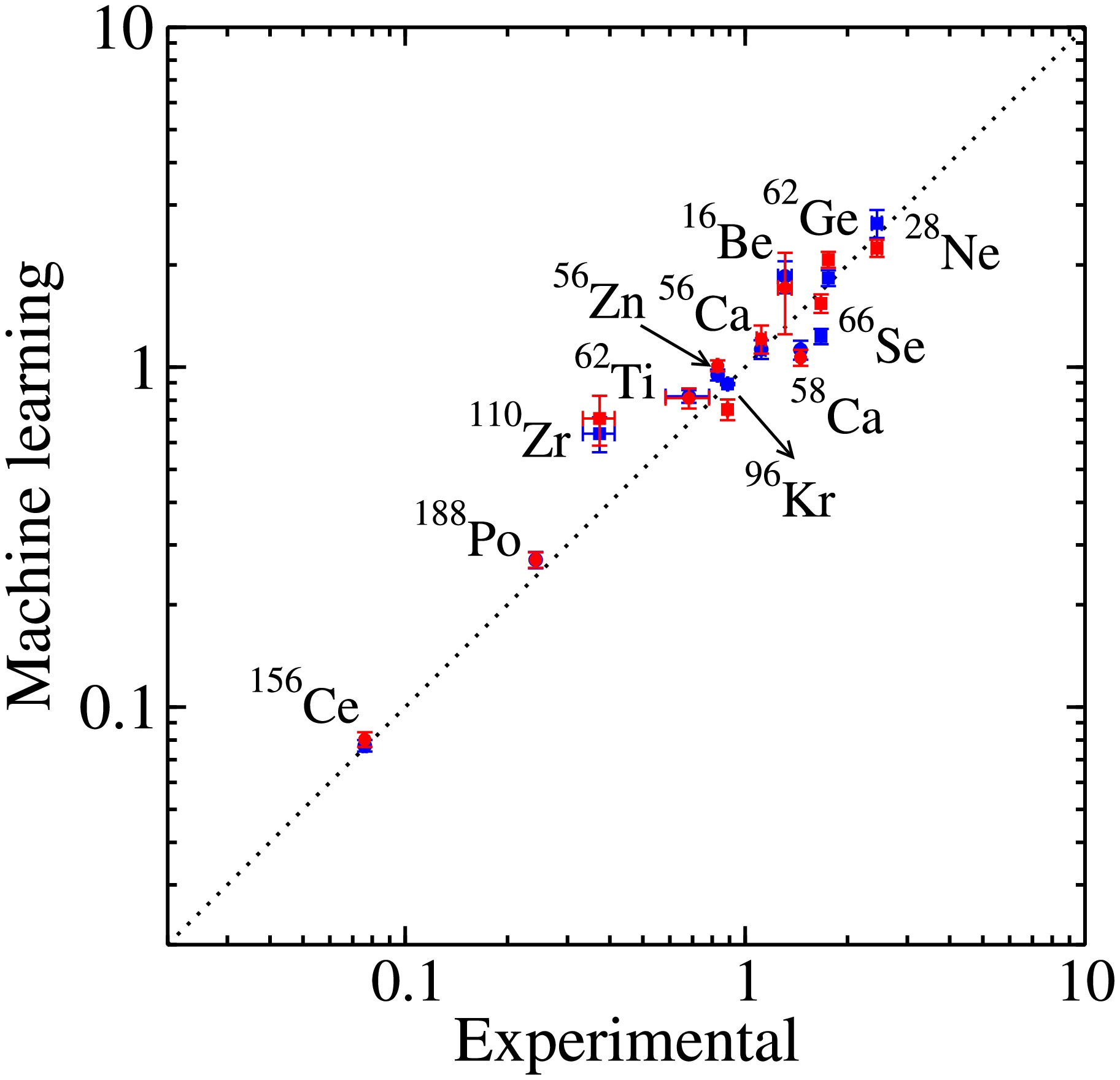

Figure 8.  (Color online) Comparing the new experimental data for $ E(2_1^+) $ and $ E(2_2^+) $ in MeV with the results from LightGBM and SVGP, the blues symbol represent the results from SVGP, while the red symbols denote the results from LightGBM. The $ E(2_1^+) $ and $ E(2_2^+) $ are shown in circles and squares, respectively.

Data-driven approaches should not only aim for predictive accuracy but also strive to uncover underlying physical patterns. In Fig. 6, the PDP curves for Z and N show pronounced slope changes near known magic numbers, indicating the model’s sensitivity to shell effects. Fig. 9(a, c) presents the variation of $ E(2_2^+) $ with Z and N, with red markers denoting cases where Z or N corresponds to a magic number. These results show that closed-shell nuclei generally have higher excitation energies. Fig. 9(b, d) shows how SHAP values vary with Z and N, reproducing the shell effects in many regions, though discrepancies remain in deformation-dominated areas—likely due to the complex nature of nuclear shapes. This indicates that the model's predictive accuracy in such regions is still lower than that in spherical nuclei. Nonetheless, these results demonstrate that the machine learning model captures not only statistical trends but also key physical features of nuclear structure.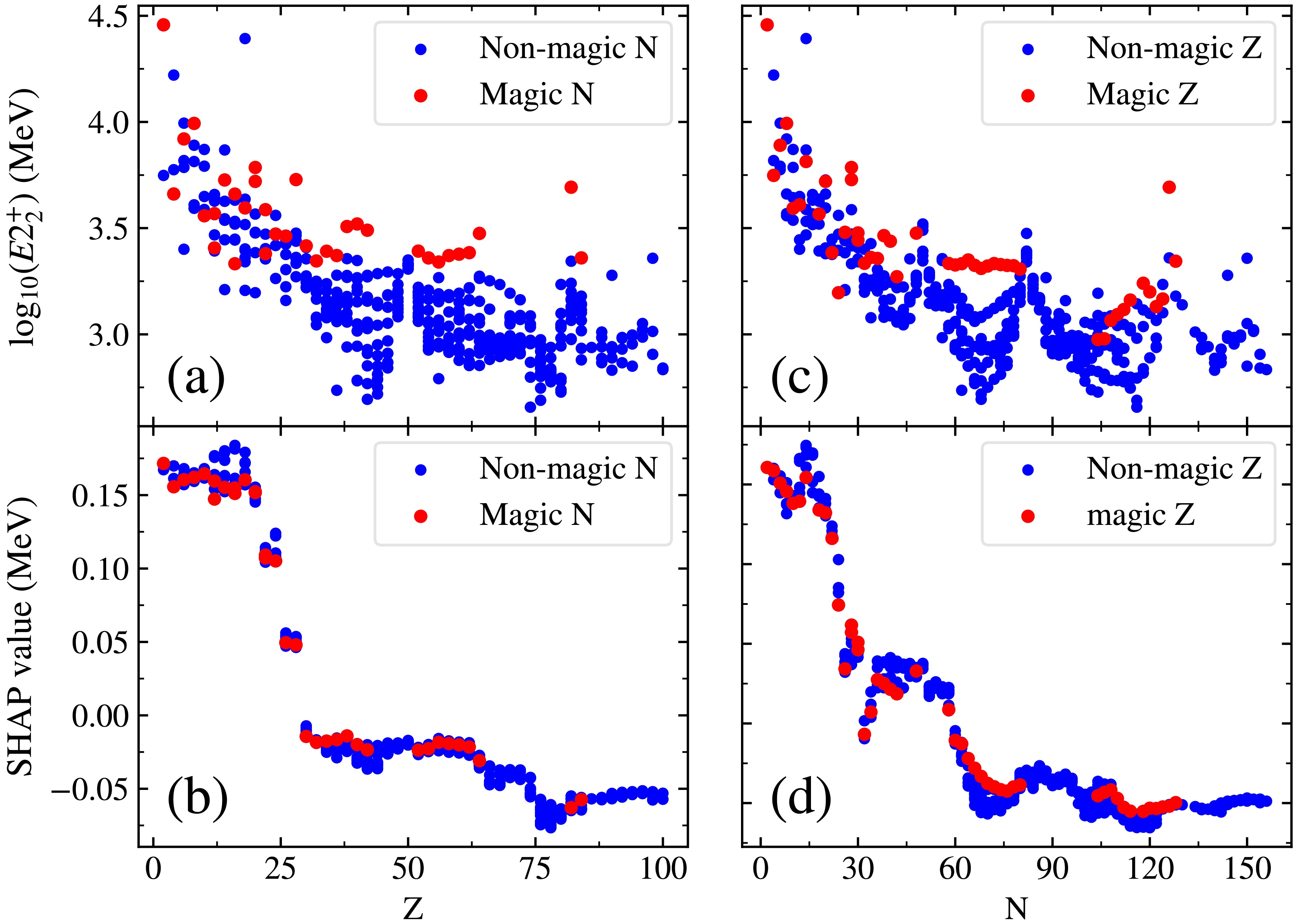

Figure 9.  (Color online) Panels (a) and (b) show the variation of $ E(2_2^+) $ energies and SHAP values with proton number Z, where red dots correspond to nuclei with neutron magic numbers, and blue dots to non-magic N. Panels (c) and (d) depict the variation of $ E(2_2^+) $ energies and SHAP values with neutron number N where red dots correspond to nuclei with proton magic numbers and blue dots represent non-magic Z.

As demonstrated that the performance of machine learning models tends to deteriorate in regions that experimental data is scare, as these algorithms are unable to learn any points in such areas. At present, we extrapolate to unmeasured nuclei for each isotope chain by considering two additional even-even nuclei. Given that ML algorithms generally exhibit reliable extrapolation abilities for nuclei that are relatively proximate to the training region and possess fast simulation speeds, it will be straightforward and easy to extend the predictions to unknown data once new experimental data are measured. In this study, despite the fact that the results from the LightGBM and SVGP can only be tested with limited new data points due to the challenges associated with measuring these far from stability line nuclei, redictions for over 300 nuclei have already been made and are included in the supplementary material [83]. Further experimental data from rare-isotope facilities like HIAF, GANIL, FAIR, FRIB, and RIKEN will be crucial for validating these extrapolated results. Additionally, this new data may provide a reference for the future experimental measurement.

Finally, to have a comprehensive study on the excitation energies of low-lying excited sates, we also trained both models to study the excitation energies of $ 2_1^+, 2_2^+, 4_1^+, 0_2^+, 0_3^+ $ states, the results are listed in the Table 2. One can see that the typical rms values obtained on the validation set are about 0.02 to 0.07 for all the states in this work, which means the differences between the experimental and theoretical results range from 1.05 to 1.17 times. This performance is significantly better than the results provided by the theoretical nuclear models. Comparing the findings with those in Ref. [57], it can be seen that the incorporating more features that contain physical information leads to smaller rms values. This is because only 5 features were used in Ref. [57], whereas our work employed more than 16 features. In addition, the rms for validation provided by SVGP is very close to that of the training set, while the rms for validation from LightGBM is larger than that of the training set. This is because LightGBM has a very deep structure, allowing it to achieve high accuracy on the training set. Overall, one can observe that we adopt state-of-the-art ML algorithms and consider a wide range of physically meaningful input features, achieving the best accuracy across multiple prediction tasks. A key strength of our approach lies in the high dimensionality of the input features, which essentially encode our current comprehensive understanding of nuclear excitation energies. The combination of high-dimensional inputs, measured experimental data, and advanced ML algorithms allows us to generate predictive results that can be compared with future experimental observations. Although the SVGP model performs slightly worse than LightGBM in terms of accuracy on certain tasks, as discussed in the manuscript, these two algorithms are fundamentally different in their design. SVGP, similar to BNN, estimates parameter distributions during training and thus provides predictive uncertainties. In contrast, LightGBM estimates uncertainty by repeatedly training on different randomly selected subsets of the data and computing the statistical distribution of predictions. Exploring low-lying excitation energies using both types of models offers complementary insights and adds valuable robustness to our investigation of the systematic behavior of excitation energies. In addition, we place great importance on the verifiability of our research and have organized and uploaded the code and datasets used in this study to a public GitHub repository: https://github.com/lzl888-afk/Study-the-yrast-and-yrare-2-states-using-machine-learning-approaches.

Energy	Number of Nuclei	Feature Number	Training Ratio	Algorithm	Training Set rms	Validation Set rms	Reference
$E(2_1^+)$	622	5	0.9	LightGBM		0.130	Ref. [57]
	629	3	0.9	BNN		0.048	Ref. [55]
	660	16	0.9	LightGBM	0.0079(4)	0.030(9)	Ref. [56]
	660	16	0.8	LightGBM	0.032(4)	0.049(5)	This work
	660	16	0.8	SVGP	0.066(2)	0.070(6)	This work
$E(4_1^+)$	594	3	0.9	BNN		0.035	Ref. [55]
	608	16	0.9	LightGBM	0.0071(1)	0.020(3)	Ref. [56]
	608	16	0.8	SVGP	0.050(2)	0.046(2)	This work
$E(2_2^+)$	437	16	0.8	LightGBM	0.040(3)	0.058(5)	This work
				SVGP	0.067(7)	0.070(6)	This work
$E(0_2^+)$	338	3	0.9	BNN		0.063	Ref. [55]
	323	16	0.8	LightGBM	0.046(3)	0.064(4)	Ref. [82]
	323	16	0.8	SVGP	0.075(4)	0.072(3)	This work
$E(3_1^-)$	316	16	0.8	LightGBM	0.035(1)	0.047(3)	Ref. [82]
				SVGP	0.050(3)	0.055(3)	This work
$E(0_3^+)$	225	16	0.8	LightGBM	0.050(2)	0.064(3)	Ref. [82]
				SVGP	0.062(3)	0.067(4)	This work

Table 2.  The average rms values for the excitation energies of $2_1^+, 4_1^+,2_2^+, 0_2^+,3_1^-, 0_3^+$ states.

In this study, the excitation energies of the $ 2_1^+ $ and $ 2_2^+ $ states for even-even nuclei were evaluated using two machine learning algorithms: LightGBM (a decision tree-based method) and SVGP (a Bayesian approach) algorithms. This is the first attempt to apply machine learning algorithms to predict $ E(2_2^+) $, marking the inaugural use of data-driven approaches for this observable. Employing the $ M16 $ feature space, the rms deviations of LightGBM and SVGP with respect to the experimental $ log_{10}E $ values are 0.049 $ \pm $ 0.005 (1.12 times) and 0.070 $ \pm $ 0.006 (1.18 times) for $ 2_1^+ $, respectively. For $ E(2_2^+) $, the rms deviations of LightGBM and SVGP with respect to the experimental $ log_{10}E $ values are 0.058 $ \pm $ 0.005 (1.14 times) and 0.077 $ \pm $ 0.006 (1.19 times), respectively. Both methodologies substantially outperform the results from the HFB+5DCH model [25], effectively capturing the behaviors of excitation energies of the $ 2_1^+ $ and $ 2_2^+ $ states over nuclear landscape. A comparative analysis between LightGBM and SVGP reveals that LightGBM consistently delivers superior performance compared to SVGP across both training and validation datasets. However, they exhibit very similar behavior on the limited new dataset. These findings underscore the potential of machine learning as a formidable alternative to traditional theoretical models for predicting excitation energies, showcasing clear and substantial success. In conclusion, our results, derived from two machine learning frameworks, not only corroborate previous studies but also establish LightGBM and SVGP as useful and effective tools for machine learning applications in nuclear physics.

The authors are grateful to the C3S2 computing center in Huzhou University for calculation support.